Two theorems of generalized unsynchronization for coupled chaotic systems

(1)

www.elsevier.com/locate/na

Two theorems of generalized unsynchronization for coupled

chaotic systems

Zheng-Ming Ge

∗

, Pu-Chien Tsen

Department of Mechanical Engineering, National Chiao Tung University, Hsinchu, Taiwan, ROC Received 13 June 2007; accepted 25 October 2007

Abstract

Generalized chaos synchronization has been widely studied and many control methods have been presented, but up to now no criterion has been given for generalized unsynchronization. The generalized unsynchronization means that the state variables of two coupled chaotic systems cannot approach generalized synchronization. In this paper, we propose two theorems which give the criteria of generalized unsynchronization for two different chaotic dynamic systems with whatever large strength of linear coupling. Two simulated examples are also given.

c

2008 Published by Elsevier Ltd

MSC:34C15; 34C28; 37D45

Keywords:Generalized unsynchronization; Chaos; Synchronization; Coupled chaotic systems

1. Introduction

In recent years, synchronization in chaotic dynamic system has been a very interesting problem and has been widely studied [1–5]. Besides, generalized synchronization also has been investigated in various fields [6–17]. Generalized synchronization means that there is a functional relation between the states of the driving system and the response system. In Section 2, we propose two theorems which give the criteria of generalized unsynchronization for two different chaotic dynamic systems with whatever large strength of linear coupling. In Section 3, the Chen system and a new chaotic system which we proposed are presented as a simulated example for the first theorem [18]. The R¨ossler system with corresponding new chaotic system proposed are presented as simulated examples for the second theorem [19]. In Section4, conclusions are given.

2. Two theorems of generalized unsynchronizability Consider the following nonautonomous systems

˙

x = f(t, x), (1)

∗_{Corresponding address: Department of Mechanical Engineering, National Chiao Tung University, 1001 Ta Hsueh Road, Hsinchu 30050,}

Taiwan, ROC. Tel.: +886 3 5712121 55119; fax: +886 3 5720634. E-mail address:[email protected](Z.-M. Ge).

0362-546X/$ - see front matter c 2008 Published by Elsevier Ltd

(2)

where x ∈ Rn, f : Ω1⊂R × Rn→Rn. Eq.(1)is considered as a master system. A slave system is given by

˙

y = g(t, y), (2)

where y ∈ Rn, g : Ω2⊂R × Rn→Rn. Both f and g satisfy Lipschitz condition. Ω1, Ω2are domains containing the

origin. Assume that the solutions of Eqs.(1)and(2)have bounds then they must exist for infinite time. Now we consider the following unidirectional nonautonomous coupled system

˙

x = f(t, x) ˙

y = g(t, y) + U(t, x, y), (3)

where U(t, x, y) is a coupled term.

Definition. The system (3) is generalized synchronized if there is a continuous function H(x) and let error e = y − H(x) s.t. limt →∞kek = 0. But, if no positive constant C can be found such that e → 0 as t → ∞ for all

ke(t0)k < C, system(3)is generalized unsynchronizable [20].

In order to discuss the generalized synchronization of x and y, define z = H(x) and error e = y − z. Error equation can be written as

˙

e = ˙y − ˙z = g(t, e + z) − ∂ H

∂xf(t, x) + U(t, z, e + z). (4)

Now the first theorem will be given for a special case of Eq.(3). Consider unidirectional coupled nonautonomous systems as

˙

x = f(t, x) ˙

y = g(t, y) + Γ (z − y), (5)

where f and g satisfy Lipschitz condition, and the Lipschitz constant of g is L. Γ ∈ Mn×nis a constant diagonal matrix

with positive entries which represents the strength of the linear coupling term z − y. Since e = y − H(x) = y − z, the error dynamic equation can be obtained as

˙

e = ˙y − ˙z = g(t, e + z) − ∂ H

∂xf(t, x) − Γ e. (6)

Let h(t, z) = ∂ H_∂xf(t, x), system(6)can be written as ˙

e = ˙y − ˙z = g(t, e + z) − h(t, z) − Γ e (7)

which is a nonautonomous system of differential equations for state e. Now we give a theorem of unsynchronizability: Theorem 1. Two different dynamic systems in Eq.(5)are unsynchronizable for however large coupling strengthΓ with positive entries, if hi(t, z) ≤ gi(t, z) (i = 1, . . . , n) in Ω1∩Ω2, and kh(t, z) − g(t, z)k > 0 except at the origin,

for any solutionz(t).

Proof. Choose a Lyapunov function V(e) = e1e2· · ·en which is positive in quadrant e1 > 0, e2 > 0, . . . , en > 0,

then ˙V along any state trajectory of system(6)becomes [21]: ˙ V = e2e3· · ·ene˙1+e1e3· · ·ene˙2+ · · · +e1e2· · ·en−1e˙n =e2e3· · ·en[g1(t, e + z) − h1(t, z) − Γ1e1] +e1e3· · ·en[g2(t, e + z) − h2(t, z) − Γ2e2] · · · +e1e2· · ·en−1[gn(t, e + z) − hn(t, z) − Γnen] =e2e3· · ·en[g1(t, e + z) − g1(t, z) + g1(t, z) − h1(t, z) − Γ1e1] + · · · +e1e2· · ·en−1[gn(t, e + z) − gn(t, z) + gn(t, z) − hn(t, z) − Γnen].

(3)

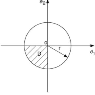
Fig. 1. D region for n = 2. When e1> 0, e2> 0, . . . , en> 0, we have ˙ V ≤ e2e3· · ·en[|g1(t, e + z) − g1(t, z)| + g1(t, z) − h1(t, z) − Γ1e1] + · · · +e1e2· · ·en−1[|gn(t, e + z) − gn(t, z)| + gn(t, z) − hn(t, z) − Γnen] ≤ e2e3· · ·en[L kek + g1(t, z) − h1(t, z) − Γ1e1] + · · ·, (8)

where |g1(t, e + z) − g1(t, z)| ≤ L kek follows the Lipschitz condition. When kek 1, the terms of lower degree of

error components e2e3· · ·en[g1(t, z) − h1(t, z)], e1e3· · ·en[g2(t, z) − h2(t, z)], . . . can be neglected when the sign

of ˙V is considered, then ˙

V ≤ e2e3· · ·en[L kek − Γ1e1] +e1e3· · ·en[L kek − Γ2e2] + · · ·. (9)

For sufficiently large Γi, ˙V can be negative in the quadrant e1 > 0, e2 > 0, . . . , en > 0. So the state point tends

to decrease ke(t)k with time when ke0k is sufficiently large. When kek 1, the proof is as follows. Now when

e1> 0, e2> 0, . . . , en> 0, ˙V is expressed as

˙

V ≥ e2e3· · ·en[− |g1(t, e + z) − g1(t, z)| + g1(t, z) − h1(t, z) − Γ1e1] + · · ·

≥ e2e3· · ·en[−L kek + g1(t, z) − h1(t, z) − Γ1e1] + · · ·. (10)

When kek 1, the terms of higher degree e2e3· · ·en[−L kek − Γ1e1], · · · can be neglected when the sign of ˙V is

considered, then ˙

V ≥ e2e3· · ·en[g1(t, z) − h1(t, z)] + e1e3· · ·en[g2(t, z) − h2(t, z)] + · · · . (11)

By the condition hi(t, z) ≤ gi(t, z) (i = 1, . . . , n) inΩ1∩Ω2, kh(t, z) − g(t, z)k > 0, fi(t, z) = gi(t, z)(i =

1, . . . , n) do not occur simultaneously. Therefore the right-hand side of above inequality is positive, i.e. ˙V is positive in region D ofFig. 1, which is the quadrant e1> 0, e2> 0, . . . , en> 0 of the neighborhood of the origin.

Choose r > 0 such that for the ball Br = {e ∈ Rn| kek ≤ r }, we have

D = {e ∈ Br|V(e) > 0} (12)

of which the boundary is the surface V(e) = 0 and the sphere kek = r. Since V (0) = 0, the origin lies on the boundary of D inside Br. The point e0is in the interior of D and V(e0) = b > 0. Now we prove that the trajectory

e(t) started at e(0) = e0must leave the set D, i.e. the trajectory must leave the neighborhood of the origin, e cannot

approach zero. To see this point, notice that as long as e(t) is inside D, V (e(t)) ≥ b since ˙V (e) > 0 in D. Let

β = min{ ˙V (e)|e ∈ D and V (e) ≥ b} (13)

which exists since the continuous function ˙V(e) has a minimum over the compact set {e ∈ D and V (e) ≥ b} = {e ∈ Br, andV (e) ≥ b} [22]. Then,β > 0 and

V(e(t)) = V (e0) + Z t 0 ˙ V(e(s))ds ≥ b + Z t 0 βds = b + βt. (14)

(4)

Fig. 2. D region for n = 2.

This inequality shows that e(t) cannot stay forever in D because V (e) is bounded on D. Now, e(t) cannot leave D through the surface V(e) = 0 since V (e(t)) ≥ b. Hence, it must leave D through the sphere kek = r, i.e. it must leave the neighborhood of the origin, e can never approach zero. Two different dynamic systems in Eq.(5) are unsynchronizable for however large Γ .

Theorem 2. Two different dynamic systems in Eq.(5)is unsynchronizable for however large coupling strengthΓ , if hi(t, z) ≥ gi(t, z)(i = 1, . . . , n) in Ω1∩Ω2, and kh(t, z) − g(t, z)k > 0 except at the origin, for any solution z(t).

Proof. Choose a Lyapunov function V(e) = e1e2· · ·en, then ˙V along any state trajectory of system(6)becomes:

Case1. When n is odd, V(e) is negative in the quadrant e1< 0, e2< 0, . . . en< 0.

˙ V = e2e3· · ·ene˙1+e1e3· · ·ene˙2+ · · · +e1e2· · ·en−1e˙n =e2e3· · ·en[g1(t, e + z) − g1(t, z) + g1(t, z) − h1(t, z) − Γ1e1] + · · · +e1e2· · ·en−1[gn(t, e + z) − gn(t, z) + gn(t, z) − hn(t, z) − Γnen]. When e1< 0, e2< 0, . . . en< 0, we have ˙ V ≥ e2e3· · ·en[− |g1(t, e + z) − g1(t, z)| + g1(t, z) − h1(t, z) − Γ1e1] + · · · +e1e2· · ·en−1[− |gn(t, e + z) − gn(t, z)| + gn(t, z) − hn(t, z) − Γnen] ≥e2e3· · ·en[−L kek + g1(t, z) − h1(t, z) − Γ1e1] + · · ·, (15)

V ≥ e2e3· · ·en[−L kek − Γ1e1] +e1e3· · ·en[−L kek − Γ2e2] + · · ·

= −e2e3· · ·en[L kek + Γ1e1] −e1e3· · ·en[L kek + Γ2e2] + · · ·. (16)

For sufficiently large Γi, ˙V can be positive in the quadrant e1 < 0, e2 < 0, . . . , en < 0. So the state point tends

to decrease ke(t)k with time when ke0k is sufficiently large. When kek 1, the proof is as follows. Now when

e1< 0, e2< 0, . . . , en < 0, ˙V is expressed as

˙

V ≤ e2e3· · ·en[|g1(t, e + z) − g1(t, z)| + g1(t, z) − h1(t, z) − Γ1e1] + · · ·

≤e2e3· · ·en[L kek + g1(t, z) − h1(t, z) − Γ1e1] + · · ·. (17)

When kek 1, the terms of higher degree e2e3· · ·en[L kek − Γ1e1], . . . can be neglected when the sign of ˙V is

considered, then ˙

V ≤ e2e3· · ·en[g1(t, z) − h1(t, z)] + e1e3· · ·en[g2(t, z) − h2(t, z)] + · · · . (18)

By the condition kh(t, z) − g(t, z)k > 0, hi(t, z) = gi(t, z)(i = 1, . . . , n) do not occur simultaneously. Therefore the

right-hand side of above inequality is negative, i.e. ˙V is negative in region D ofFig. 2, which is the quadrant e1< 0,

(5)

Choose r > 0 such that for the ball Br = {e ∈ Rn| kek ≤ r }, we have

D = {e ∈ Br|V(e) < 0}. (19)

By the similar reasoning as that in the latter part of the proof forTheorem 1, we can prove that the state trajectory started from D must leave the neighborhood of the origin, e can never approach zero. Two different dynamic systems in Eq.(5)are unsynchronizable for however large Γ .

Case2. When n is even, V(e) is positive in the quadrant e1< 0, e2< 0, . . . , en< 0.

˙ V = e2e3· · ·ene˙1+e1e3· · ·ene˙2+ · · · +e1e2· · ·en−1e˙n =e2e3· · ·en[g1(t, e + z) − g1(t, z) + g1(t, z) − h1(t, z) − Γ1e1] + · · · +e1e2· · ·en−1[gn(t, e + z) − gn(t, z) + gn(t, z) − hn(t, z) − Γnen]. When e1< 0, e2< 0, . . . , en < 0, we have ˙ V ≤ e2e3· · ·en[− |g1(t, e + z) − g1(t, z)| + g1(t, z) − h1(t, z) − Γ1e1] + · · · +e1e2· · ·en−1[− |gn(t, e + z) − gn(t, z)| + gn(t, z) − hn(t, z) − Γnen] ≤ e2e3· · ·en[−L kek + g1(t, z) − h1(t, z) − Γ1e1] + · · ·, (20)

V ≤ e2e3· · ·en[−L kek − Γ1e1] +e1e3· · ·en[−L kek − Γ2e2] + · · ·

= −e2e3· · ·en[L kek + Γ1e1] −e1e3· · ·en[L kek + Γ2e2] + · · ·. (21)

For sufficiently large Γi, ˙V can be negative in the quadrant e1 < 0, e2 < 0, . . . , en < 0. So the state point tends to

decrease ke(t)k with time when ke0k is sufficiently large. When kek 1, the proof is as follows. Now when e1< 0,

e2< 0, . . . , en< 0, ˙V is expressed as

˙

V ≥ e2e3· · ·en[|g1(t, e + z) − g1(t, z)| + g1(t, z) − h1(t, z) − Γ1e1] + · · ·

≥ e2e3· · ·en[L kek + g1(t, z) − h1(t, z) − Γ1e1] + · · ·. (22)

When kek 1, the terms of higher degree e2e3· · ·en[L kek − Γ1e1], · · · can be neglected when the sign of ˙V is

considered, then ˙

V ≥ e2e3· · ·en[g1(t, z) − h1(t, z)] + e1e3· · ·en[g2(t, z) − h2(t, z)] + · · · (23)

By the condition kh(t, z) − g(t, z)k > 0, hi(t, z) = gi(t, z)(i = 1, . . . , n) do not occur simultaneously. Therefore

the right-hand side of above inequality is positive, i.e. ˙V is positive in region D ofFig. 2which is the quadrant e1< 0,

e2< 0, . . . , en< 0 of the neighborhood of the origin.

By the same reasoning as that in the latter part of the proof forTheorem 1, we can prove that the state trajectory started from the neighborhood of the origin in the quadrant e1< 0, e2< 0, . . . , en< 0 must leave the neighborhood

and can never approach zero. Two different dynamic systems in Eq.(5)are unsynchronizable for however large Γi.

3. Simulated examples

An example for the first theorem is Chen system with a new chaotic system proposed. Consider the following unidirectional coupled systems:

˙ x = a(y − x) ˙ y =(c − a)x − xz + cy ˙ z = x y − bz (24a) ˙˜x = a( ˜y − ˜x) + sin2_{x −}_˜ _{γ e} 1 ˙˜y =(c − a) ˜x − ˜x ˜z + c ˜y + ˜x2₋_{γ e} 2 ˙˜z = ˜x ˜y − b˜z + ˜x2₋_{γ e} 3 (24b)

(6)

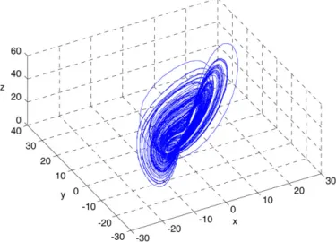
Fig. 3. Chaotic attractor for the Chen system(24a), with a = 35, b = 3 and c = 28, initial condition (0.5, 1, 5).

Fig. 4. Lyapunov exponent for the Chen system(24a), with b = 3 and c = 28, initial condition (0.5, 1, 5).

e = y − z, z = H(x) = Ax + b A =   1 0 0 0 1 0 0 0 1  , b =   3 5 7  ,

whereγ = 1000 which is sufficiently large. Eq.(24a)is the Chen system and Eq.(24b)without coupling is a new chaotic system which we proposed. The chaotic attractor and Lyapunov exponent diagrams for systems(24a)and

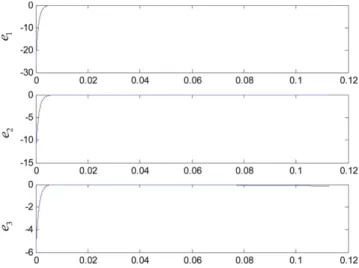
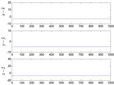
(24b)without coupling term are shown inFigs. 3–6. For initial states (0.5, 1,5), (30, 20, 18) and system parameters a =35, b = 3 and c = 28, three state errors and error versus time are shown inFigs. 7–9.Fig. 8shows that errors decreases with time when error is large, but one can clearly find inFig. 9that the errors cannot approach zero as time evolves.

An example for the second theorem is the R¨ossler system with a new chaotic system proposed. Consider the following unidirectional coupled systems with linear coupling in the form of Eq.(5):

˙ x = −y − z ˙ y = x + ay ˙ z = b + z(x − c) (25a)

(7)

Fig. 5. Chaotic attractor for the chaotic system(24b), with a = 35, b = 3 and c = 28, initial condition (30, 20, 18).

Fig. 6. Lyapunov exponent for the chaotic system(24b), with b = 3 and c = 28, initial condition (30, 20, 18).

(8)

Fig. 8. Error versus time for unidirectional coupled systems(24), with a = 35, b = 3 and c = 28, initial conditions (0.5, 1,5), (30, 20, 18).

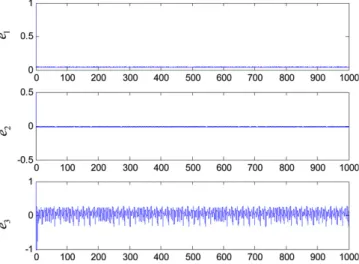
Fig. 9. Error versus time for unidirectional coupled systems(24), with a = 35, b = 3 and c = 28, initial conditions (0.5, 1, 5), (30, 20, 18).

˙˜x = − ˜y − ˜z − sin2_{y −}_{γ e} 1

˙˜y = ˜x + a ˜y − sin2_{y −}_{γ e} 2 ˙˜z = b + ˜z( ˜x − c) − sin2_{z −}_˜ _{γ e} 3 (25b) e = y − z, z = H(x) = Ax + b A =   1 0 0 0 1 0 0 0 1  , b =   3 5 7  ,

whereγ = 300. The Lyapunov exponent diagrams for systems(25a)and(25b)without coupling term are shown in

Figs. 10and11. For initial states (20, 10, 25), (2.5, 2, 2.5) and system parameter a = 0.2, b = 0.2 and c = 5.7, three state errors and errors versus time are shown inFigs. 12–14.Fig. 13shows that errors decreases with time when error is large, but one can clearly find inFig. 14that the errors cannot approach zero as time evolves.

4. Conclusions

In this paper, two theorems are proposed. They give the criteria of generalized unsynchronization for two different chaotic dynamic systems with whatever large strength of linear coupling. The Chen system and the R¨ossler system

(9)

Fig. 10. Lyapunov exponent for the R¨ossler system(25a), with b = 0.2 and c = 5.7, initial condition (20, 10, 25).

Fig. 11. Lyapunov exponent for the chaotic system(25b), with b = 0.2 and c = 5.7, initial condition (2.5, 2, 2.5).

Fig. 12. State errors versus time for unidirectional coupled systems(25), with a = 0.2, b = 0.2 and c = 5.7, initial conditions (20, 10, 25), (2.5, 2, 2.5).

(10)

Fig. 13. Error versus time for unidirectional coupled systems(25), with a = 0.2, b = 0.2 and c = 5.7, initial conditions (20, 10, 25), (2.5, 2, 2.5).

Fig. 14. Errors versus time for unidirectional coupled systems(25), with a = 0.2, b = 0.2 and c = 5.7, initial conditions (20, 10, 25), (2.5, 2, 2.5).

with two corresponding new chaotic systems proposed are used as simulation examples which effectively confirm the theorems.

Acknowledgment

This research was supported by the National Science Council, Republic of China, under Grant No. NSC95-2212-E-009-175.

References

[1] L.M. Pecora, T.L. Carroll, Synchronization in chaotic systems, Phys. Rev. Lett. 64 (1990) 821.

[2] R. He, P.G. Vaidya, Analysis and synthesis of synchronous periodic and chaotic systems, Phys. Rev. A 46 (1992) 7387. [3] M. Ding, Ott, Enhancing synchronism of chaotic systems, Phys. Rev. E 49 (1994) 945.

[4] K. Murali, M. Lakshmanan, Drive-response scenario of chaos synchronization in identical nonlinear systems, Phys. Rev. E 49 (1994) 4882. [5] L. Kocarev, U. Parlitz, R. Brown, Robust synchronization of chaotic systems, Phys. Rev. E 61 (2000) 3716.

[6] T.-L. Liao, S.-H. Tsai, Adaptive synchronization of chaotic systems and its application to secure communications, Chaos Solitons Fractals 11 (2000) 1387.

[7] S. Chen, J. Lu, Chaos synchronization of an uncertain unified chaotic system via adaptive control, Chaos Solitons Fractals 14 (2002) 643. [8] M. di Bernardo, A purely adaptive controller to synchronize and control chaotic systems, Phys. Lett. A 214 (1996) 139.

(11)

[9] J.-Q. Fang, Y.-G. Hong, G.-R. Chen, Switching manifold approach to chaos synchronization, Phys. Rev. E 59 (1999) R2523. [10] X.-H. Yu, Y.-X. Song, Chaos synchronization via controlling partial state of chaotic systems, Internat. J. Bifur. Chaos 11 (2001) 1737. [11] Zheng-Ming Ge, W.-Y. Leu, Anti-control of chaos of two-degrees-of-freedom loudspeaker system and chaos synchronization of different

order systems, Chaos Solitons Fractals 20 (2004) 503.

[12] Zheng-Ming Ge, C.-C. Chen, Phase synchronization of coupled chaotic multiple time scales systems, Chaos Solitons Fractals 20 (2004) 639. [13] Zheng-Ming Ge, C.-M. Chang, Chaos synchronization and parameters identification of single time scale brushless DC motors, Chaos Solitons

Fractals 20 (2004) 883.

[14] Zheng-Ming Ge, W.-Y. Leu, Chaos synchronization and parameter identification for loudspeaker systems, Chaos Solitons Fractals 21 (2004) 1231.

[15] Y. Yu, S. Zhang, The synchronization of linearly bidirectional coupled chaotic systems, Chaos Solitons Fractals 22 (2004) 189. [16] C. Li, X. Liao, Complete and lag synchronization of hyperchaotic systems using small impulses, Chaos Solitons Fractals 22 (2004) 857. [17] Zheng-Ming Ge, Yen-Sheng Chen, Synchronization of unidirectional coupled chaotic systems via partial stability, Chaos Solitons Fractals 21

(2004) 101.

[18] G Chen, T Ueta, Yet another chaotic attractor, Internat. J. Bifur. Chaos 9 (1999) 1465. [19] O.E. R¨ossler, An equation for continuous chaos, Phys. Lett. A 57 (1976) 397.

[20] Zheng-Ming Ge, Pu-Chien Tsen, The theorems of unsynchronizability and synchronization for coupled chaotic systems, Int. J. Nonlinear Sci. Numer. Simul. 8 (2007) 101.

[21] Zheng-Ming Ge, Developing Theory of Motion Stability, Gau Lih Book Company, Taipei, 2001. [22] T.M. Apostol, Mathematical Analysis, Addison-Wesley, Reading, MA, 1957.