國
立
交
通
大
學
電機與控制工程學系
碩
士
論
文
MPEG-2/4
低複雜度先進音訊編碼演算
法最佳化及在 StrongARM 平台上之實現
MPEG-2/4 LOW COMPLEXITY
AAC
ENCODER OPTIMIZATION AND
IMPLEMENTATION ON A StrongARM
PLATFORM
研 究 生 : 林映伶
指導教授 : 吳炳飛 教授
MPEG-2/4 低複雜度先進音訊編碼演算法
最佳化及在 StrongARM 平台上之實現
研 究 生 : 林映伶
Student : Yin-Ling Lin
指導教授 : 吳炳飛 教授
Advisor : Prof. Bing-Fei Wu
國立交通大學
電機與控制工程學系
碩士論文
A Thesis
Submitted to Department of Electrical and Control Engineering
College of Electrical Engineering and Computer Science
National Chiao Tung University
In Partial Fulfillment of the Requirements
For the Degree of Master
In
Electrical and Control Engineering
July 2005
Hsinchu, Taiwan, Republic of China
MPEG-2/4 低複雜度先進音訊編碼演算
法最佳化及在 StrongARM 平台上之實現
研究生 : 林映伶
指導教授 : 吳炳飛 教授
國立交通大學電機與控制工程學系碩士班
摘要
這篇論文提出一套 AAC 編碼的最佳化演算法以及在 AAC 編碼系統中加入 資料嵌入演算法的應用。最後將這兩套系統實現在一顆 206 MHz 的 32 位元定點 處理器 StrongARM SA-1110 上。實驗結果顯示,我們所提出的架構在實驗平台 上可執行至少一倍速的壓縮。在 AAC 編碼最佳化中,我們移除計算量龐大的長 短窗轉換,簡化 TNS 及 M/S 立體聲編碼的控制流程,數學函式的簡化運算及較 快速的量化模組,在 MDCT 的實現方式上,也採用了以快速演算法。為了彌補 定點化過程中所產生的誤差,我們加入了頻寬控制及動態精確度的 MDCT 運算 等。最後,為了進一步增加 AAC 檔案的功能性,並在 AAC 編碼系統中加入資 料嵌入的應用。MPEG-2/4 LOW COMPLEXITY AAC
ENCODER OPTIMIZATION AND
IMPLEMENTATION ON A StrongARM
PLATFORM
Student : Yin-Ling Lin
Advisor : Prof. Bing-Fei Wu
Department of Electrical and Control Engineering
National Chiao Tung University
A
BSTRACT
In this thesis, we present an optimized AAC encoding scheme and also proposed a data embedded method integrated into AAC encoding system. Both of them are finally realized on a 32-bit fixed-point processor, StrongARM SA-1110. Experimental result shows that at least 1 encoding speed is achieved. In the AAC encoding algorithm, we propose several approaches including the removal of block switching, fast MDCT, simplified TNS, simplified M/S stereo coding, mathematical function optimization and fast quantization. To compensate the error caused by fixed-point conversion, a bandwidth control and a dynamic data precision MDCT are applied. Finally, a data embedded method is implemented to further increase its utility.
ACKNOWLEDGEMENTS
首先,要感謝我的指導教授吳炳飛老師,這兩年來在研究方式及研究態度上 的指導,讓我受益良多。尤其提供了一個資源充足的研究環境,找到我想做的東 西,還有參賽寫書的經驗,都是我在進研究所之前所沒想過的。也許進交大念研 究所並不在我原先一直以為的人生規劃表上,但真的很感恩目前為止經歷過的一 切,很感謝吳老師給我的機會。 此外,最要感謝的是旭哥,不但常在學術研究上給我很多的建議,上班後仍 然很有義氣的帶我們 meeting 到畢業。還有在進入音訊編碼領域幫忙很多的鐵男 學長,教導實現資料嵌入的榮煌學長,在系統上幫忙很多的俊傑,剛進研究所常 載我上下學的螞蟻學姐,及常請大家吃水果的飛鼠學姐。 當然不能不提的是一起八卦、shopping 的好姐妹,元馨學妹,一起吃飯、 玩樂、幫忙搬家的培恭、晏阡及學弟小熊、宗堯,煮咖啡老歌同好重甫學長,還 有幫忙買電腦的子萱學弟,一起做實驗的皓昱學弟。如果沒有你們,我的研究所 生活一定會單調許多吧! 最後,最要感謝的是一直支持著我的父母、姐姐,提供我很好的生活條件, 讓我可以無後顧之憂的專心學業。還有把我像親生女兒一樣照顧的新竹親戚,大 姑姑、和英阿姨。還有許多感謝無法一一列述,謹以這篇論文獻給所有在研究生 涯幫助過我的人,謝謝你們! 林映伶 民國九十四年七月 於新竹CONTENTS
ABSTRACT(CHINESE) ...i ABSTRACT(ENGLISH)...ii ACKNOWLEDGEMENTS ... iii CONTENTS...iv LIST OF TABLES...viiLIST OF FIGURES ...vii
CHAPTER 1. Introduction ...1
1.1 Background ...1
1.2 Motivation...1
1.3 Innovation ...2
1.4 Content Organization ...2
CHAPTER 2. Psychoacoustic Model...3
2.1 The Absolute Threshold of Hearing...3
2.2 Critical Band ...4
2.3 Masking Effect...6
2.3.1 Simultaneous Masking...6
2.3.2 Temporal Masking ...7
2.4 Psychoacoustic Model ...7
CHAPTER 3. MPEG-2 AAC Algorithm...10
3.1 Overview...10
3.2 Filter Bank and Block Switching...14
3.2.1 MDCT ...15
3.2.2 Window Shape ...16
3.2.3 Block Switching...18
3.3 Temporal Noise Shaping...21
3.3.1 Pre-echo Phenomenon ...21
3.3.2 TNS Processing...23
3.4 M/S Stereo Coding...24
3.4.1 Binaural Masking Level Difference...25
3.4.2 M/S Stereo Threshold ...26
3.4.3 L/R and M/S Switching ...28
3.5 Intensity Stereo Coding...28
3.6 Prediction ...29
3.6.1 Predictor Structure ...30
3.6.2 Predictor Control...32
3.7.1 Nonuniform Quantization Function...33
3.7.2 Scalefactor Band ...34
3.7.3 Iteration Process...34
3.8 Noiseless Coding ...40
3.8.1 Grouping and Interleaving ...40
3.8.2 Spectral Clipping ...41
3.8.3 Huffman Coding ...42
3.8.4 Sectioning ...43
3.9 Gain Control...44
3.9.1 Polyphase Quadrature Filter ...44
3.9.2 Gain Detector ...44
3.9.3 Gain Modifier...45
3.10 Bitstream Format ...45
CHAPTER 4. MPEG-2/4 LC AAC Encoder Optimization...48
4.1 Complexity Analysis...48
4.2 Removal of Block Switching ...49
4.3 Fast MDCT ...49
4.4 Simplified TNS ...51
4.5 Simplified M/S Stereo Coding...55
4.6 Quantization Optimization...58 4.6.1 Scalefactor Prediction ...60 4.6.2 Simplified QuantizeBand() ...61 4.7 Math Function...62 4.7.1 TNS ...62 4.7.2 Quantization...63
CHAPTER 5. Implementation on a StrongARM Processor ...69
5.1 Implementation Flow ...69
5.2 Fixed-point C Code Implementation ...70
5.3 Modify Coding Style...73
CHAPTER 6. Implementation of Data Embedded Method...74
6.1 The Properties of Data Embedded Method...74
6.2 Implementation of Data Embedded Encoder ...76
6.2.1 Embedding Data into High Frequency Range ...77
6.3 Implementation of Data Embedded Decoder...79
CHAPTER 7. Experimental Results...81
7.1 MPEG-2/4 LC AAC Encoder ...81
7.1.1 Resource Distribution ...81
7.1.3 Encoding Speed ...83
7.1.4 Quality Evaluation ...84
7.2 Data Embedded Method ...85
7.2.1 Resource Distribution ...85
7.2.2 Encoding Speed and File Size...85
7.2.3 Embedded Data Size ...86
7.2.4 Quality Evaluation ...87
CHAPTER 8. Conclusions and Future Works ...89
8.1 Conclusions...89
8.2 Future Works...90
REFERENCE ...92
APPENDIX A. Advantech PCM-7130 SBC ...97
APPENDIX B. Data Embedded Codec...100
B.1 Package File ...100
B.2 Data Stream Analyzer...103
B.3 Lyrics Analyzer ...104
LIST OF TABLES
Table 2. 1 Critical bands. Fc – center frequency of the critical band ...5
Table 3. 1 MPEG-2 AAC sampling frequencies and maximum data rates...10
Table 3. 2 Tools used by three profiles ...14
Table 3. 3 Optimum Coding Methods for Extreme Input Signal Characteristics ...23
Table 3. 4 Reset groups of predictors...32
Table 4. 1 Distribution of resources in AAC-LC encoder ...48
Table 4. 2 the percentage of TNS being active ...52
Table 4. 3 Distribution of resources in TNS module (TNS is finally “ON” case)...52
Table 4. 4 Comparisons between original and modified TNS ...54
Table 4. 5 The percentage that encoder switching to M/S mode ...55
Table 4. 6 Average iteration loop count of quantizer ...60
Table 4. 7 The distribution of input range of QuantizeBand()...61
Table 4. 8 The relationship between x and 1/4b...64
Table 5. 1 Some desired bitrate and corresponding cut-off frequency of bandwidth control module ...73
Table 6. 1 Classification of the watermarking technique in this thesis...74
Table 7. 1 Distribution of resources in proposed AAC-LC encoder...82
Table 7. 2 Comparing the resource requirement with the ISO source code ...83
Table 7. 3 Encoding speed ...83
Table 7. 4 The objective test results of proposed encoder ...84
Table 7. 5 Resource distribution of the proposed encoder plus data embedded method ...85
Table 7. 6 The resulting file size and encoding speed before and after data embedded method presented ...86
Table 7. 7 The embedded bits count of different files...86
Table 7. 8 The objective test results of proposed encoder plus data embedded feature ...88
LIST OF FIGURES
Fig. 2. 1 The absolute threshold of hearing ...4
Fig. 2. 2 Idealized critical band filterbank ...5
Fig. 2. 3 An example of simultaneous masking ...6
Fig. 2. 4 Schematic representation of temporal masking effect...7
Fig. 2. 5 Block diagram of psychoacoustic model...9
Fig. 3. 3 Example of window shape switching process ...17
Fig. 3. 5 Pre-echo phenomenon example...22
Fig. 3. 6 Comparisons of input (solid) and coding noise (dashed) spectrum...24
Fig. 3. 7 Illustration of the situation in which BMLD occurs...26
Fig. 3. 8 BMLD protection ratio (bmax)...27
Fig. 3. 9 signal flow of an intensity stereo coding / decoding scheme ...29
Fig. 3. 10 The second-order backward-prediction lattice structure ...31
Fig. 3. 11 Block diagram of prediction unit for one scale factor band ...33
Fig. 3. 12 A simplified block diagram of iteration process...35
Fig. 3. 13 A simplified block diagram of inner iteration loop...37
Fig. 3. 14 A simplified block diagram of outer iteration loop...40
Fig. 3. 15 Example for short window grouping ...40
Fig. 3. 16 Spectral order within one group before interleaving ...41
Fig. 3. 17 Spectral order after interleaving ...41
Fig. 3. 18 Block Diagram of AAC encoder gain control module ...45
Fig. 4. 1 Original TNS implementation flow ...51
Fig. 4. 2 Modified TNS implementation flow ...53
Fig. 4. 3 Energy ratio of channel pair of the scalefactor band switches to M/S mode 57 Fig. 4. 4 Energy ratio of channel pair of the scalefactor band remains in L/R mode ..57
Fig. 4. 5 The flowchart of the proposed M/S stereo decision scheme ...58
Fig. 4. 6 The relationship between ABR encoding and single loop quantization ...59
Fig. 4. 7 The error magnitude of the approximating QuantizeBand() function ...62
Fig. 4. 8 The curve of nature logarithm ...66
Fig. 5. 1 Implementation Flow...70
Fig. 5. 2 Dynamic precision FFT calculation in MDCT module ...71
Fig. 6. 1 The structure of data embedded AAC encoder………...….….. 76
Fig. 6. 2 The structure of package file ...77
Fig. 6. 3 The implementation flow of data embedded method……….89
Fig. 6. 5 The implementation flow of data embedded decoding process...80
Fig. A. 1 The appearance of the Advantech PCM-7130 SBC...97
Fig. A. 2 Advantech PCM-7130 SBC ...99
Fig. B. 1 The structure of package file...101
Fig. B. 2 The flowchart of generating package file ...102
Fig. B. 3 The flowchart of data stream analyzer...104
Fig. B. 4 The flowchart of lyrics analyzer ...106
Fig. B. 5 An example of lyrics file format ...107
CHAPTER 1. Introduction
1.1 Background
With the rapid development of computer science, our life style has been changed a lot in recent years. Data are digitalized and distributed through Internet, wireless, and communication. Due to the limited bandwidth or storage space, data compression has become an important issue. Focusing on audio field, lots of audio codecs have been proposed in past years. For example, MPEG-1 layer III, generally known as MP3, has gained its popularity. Though there still has the vagueness of legalization, one can not deny that digital audio will gradually replace the traditional music market seems to be an irresistible trend.
1.2 Motivation
We’ve seen the wildly popularity of MP3 format. The request for higher coding efficiency and multichannel support drives the development of AAC format. As compared to MP3, AAC provides higher-quality results with smaller file sizes, higher resolution and multichannel support. AAC proves itself worthy of replacing MP3 as the new Internet audio standard.
Because of its superior performance and quality, AAC also constitutes the kernel of MPEG-4 audio and has been adopted in several application areas as Internet streaming, ISDN music transmission, high definition television (HDTV), satellite and
terrestrial digital audio broadcasting and for audio transmission in third generation mobile networks (as 3GPP and 3GPP2 for UMTS/CDMA2000). Especially, Apple Computer, arms with its cool devices and online music store, spares no efforts to promote AAC format. AAC is gaining its importance in the market.
1.3 Innovation
Most AAC encoders are restricted to PC-based applications, since it consumes too much computational resources to implement on portable devices which often powered by batteries.
In this thesis, we present an optimized AAC encoding algorithm which can be implemented on power-limited portable systems. An additional functionality of data embedded technique is also presented. Finally, this proposed AAC encoding algorithm with data embedding feature is realized with a 206MHz 32-bit RISC CPU, Intel® StrongARM SA-1110. At least 1X encoding speed is achieved.
1.4 Content Organization
There are 7 chapters in this thesis. Chapter 2 and Chapter 3 briefly explain the AAC encoding algorithm. Chapter 2 focuses on psychoacoustic model and chapter 3 discusses the remaining modules. Chapter 4 describes our proposed optimization for MPEG-2 low complexity (LC) profile AAC. Chapter 5 illustrates the implementation of this modified MPEG-2 LC AAC encoder with Intel® StrongARM SA-1110 RISC CPU. A data embedded method specific to AAC file is also realized, and this is described in Chapter 6. The final experimental results can be found in Chapter 7.
CHAPTER 2. Psychoacoustic Model
Most current audio coders achieve compression by exploiting the fact that “irrelevant” information is not detectable in general case. Irrelevant information is identified by incorporating several psychoacoustic principles.
2.1 The Absolute Threshold of Hearing
The absolute threshold of hearing, also called the quiet threshold, can be described as the amount of energy needed in a pure tone such that it can be detected by a listener in a noiseless environment. It is well approximated [18] by the nonlinear function: ) ( 1000 10 5 . 6 1000 64 . 3 ) ( 4 3 3 . 3 1000 6 . 0 8 . 0 2 SPL dB f e f f T f q ⎟ ⎠ ⎞ ⎜ ⎝ ⎛ + − ⎟ ⎠ ⎞ ⎜ ⎝ ⎛ = ⎟⎠ − ⎞ ⎜ ⎝ ⎛ − − − (2.1)
It is the representative of a young listener with acute hearing. When Tq( f)is applied to signal compression, it can be interpreted as a maximum allowable energy level for coding distortions introduced in frequency domain. Fig. 2.1 shows the curve of the absolute threshold of hearing.
Fig. 2. 1 The absolute threshold of hearing [17]
The sound pressure level (SPL) is a measurement of sound intensity which is calculated as Number of decibels = ⎟⎟ ⎠ ⎞ ⎜⎜ ⎝ ⎛ 0 1 10 log 10 I I (2.2) where,
I0 is the reference intensity,
The most commonly used reference intensity is 10-12 (W/m2) [8]. I1 is the intensity to be measured.
2.2 Critical Band
It turns out that a frequency-to-place transformation takes place in the inner ear, along the basilar membrane. Distinct regions in the cochlea, each with a set of neural receptors, are responsible for a limited range of frequencies. This limited frequency resolution can be expressed in terms of “critical band”. From the experimental sense, critical bandwidth can be loosely defined as the bandwidth at which subjective
domain. Table 2.2 illustrates the nonuniform Hertz spacing of the critical band. Band NO. Fc(Hz) Bandwidth(Hz) Band NO. Fc(Hz) Bandwidth(Hz) 1 50 0-100 14 2150 2000-2320 2 150 100-200 15 2500 2320-2700 3 250 200-300 16 2900 2700-3150 4 350 300-400 17 3400 3150-3700 5 450 400-510 18 4000 3700-4400 6 570 510-630 19 4800 4400-5300 7 700 630-770 20 5800 5300-6400 8 840 770-920 21 7000 6400-7700 9 1000 920-1080 22 8500 7700-9500 10 1170 1080-1270 23 10500 9500-12000 11 1370 1270-1480 24 13500 12000-15500 12 1600 1480-1720 13 1850 1720-2000
Table 2. 1 Critical bands. Fc – center frequency of the critical band [16]
2.3 Masking Effects
Masking refers to a process where one sound turns out to be inaudible because of the presence of another sound. There are two types of masking: simultaneous masking and temporal masking.
2.3.1 Simultaneous Masking
Simultaneous masking occurs in frequency domain, thus it is also called frequency masking. A simplified explanation of the mechanism is as follows: The presence of a strong signal (masker) creates an excitation of sufficient strength on the basilar membrane at the critical band location to effectively block the transmission of a weaker signal (maskee) [19]. This phenomenon has been observed both within a single critical band and between critical bands. The latter one is also known as the spread of masking. Fig. 2.3 gives an example of simultaneous masking with a masker at 150Hz.
2.3.2 Temporal Masking
Masking effect is also happened in time domain which is called the temporal masking or nonsimultaneous masking. It is the term describing those situations where sounds are hidden due to maskers which have just disappeared (this is also called post-masking), or maskers which are about to appear (this is also called pre-masking). In the context of audio signal analysis, abrupt signal transients often creates pre-masking and post-masking regions in time during which a listener will not perceive signals beneath the elevated audibility thresholds produced by a masker.
Fig. 2. 4 Schematic representation of temporal masking effect [16]
2.4 Psychoacoustic Model
The MPEG audio algorithm compresses the audio data in large part by removing the acoustically irrelevant parts of the audio signal. Psychoacoustic model (PM) exploits the masking effect of the human auditory system to calculate maximum allowable amount of quantization noise. This maximum level is referred to masking threshold. PM also uses this information along with input signal to decide bit
allocation and block type switching.
The psychoacoustic model used for AAC system is similar to the one used in MPEG-1 audio [1]. The simplified description of its process is as follows:
1. Performing a 2048-point or 256-point FFT.
2. Using FFT-transformed spectrum to calculate the unpredictability measure. 3. Calculating the threshold (part I) by input signal energy and considering the quiet
threshold.
4. Computing perceptual entropy (PE) to determine which block size (long or short) to use.
5. Calculating the minimum of masking threshold (part II) of each scalefactor band (see Section 3.6.2).
6. Calculating the signal-to-mask ratio (SMR) for each scalefactor band, and sending them to the quantizer.
The outputs from the psychoacoustic model are:
1. A set of signal-to-mask ratios and thresholds.
2. The delayed time domain data (PCM samples), which re-used by the MDCT. 3. The block type for the MDCT.
4. An estimation of how many bits should be used for encoding in addition to the average bits.
Fig. 2. 5 Block diagram of psychoacoustic model [2]
For more details about how psychoacoustic model implements, please see [2]. Delay threshold, blocktype, PE by one block
if ( window_sequence(n) == EIGHT_SHORT_SEQUENCE &&
window_sequence(n-1) == ONLY_LONG_SEQUENCE) window_sequence(n-1) == LONG_START_SEQUENCE; Calculate threshold (Part II)
Output buffer: block type, threshold, perceptual entropy, time signal Use short block
N
PE > switch_pe ?Calculate unpredictability measure
Calculate threshold (Part I)
Calculate perceptual entropy (PE)
Calculate threshold (short)
FFT
Delay compensation for filterbank Input buffer
Use long block
CHAPTER 3. MPEG-2 AAC Algorithm
3.1 Overview
Started in 1994, the ISO/IEC MPEG-2 advanced audio coding (AAC) system was designed to provide best audio quality without any restrictions due to compatibility requirements. It was finalized as an international standard in 1997 April (ISO/IEC 13818-7). The MPEG-2 AAC scheme also constitutes the kernel of the MPEG-4 audio standard. All profiles (will be introduced later) defined in MPEG-2 AAC also appear in MPEG-4 standard.
AAC can include 48 full-bandwidth audio channels in one stream plus 15 low frequency enhancement (LFE, limited to 120 Hz) channels. The sampling rates supported by the AAC system vary from 8 to 96 kHz, as shown in Table 3.1.
Sampling Frequency (Hz) Maximum Bitrate Per Channel (kbit/s)
96000 576 88200 329.2 64000 384 48000 288 44100 264.6 32000 192 24000 144 22050 132 16000 96 12000 72 11025 66.25 8000 48
The basic structure of the MPEG-2 AAC system is shown in Fig. 3.1 and Fig. 3.2. We can briefly describe the AAC encoder process as follows. First, a filter bank is used to decompose the input signal into spectral components. Based on the input signal, an estimate of current signal-to-mask ratio is computed by psychoacoustic model, which will be utilized in quantization stage in order to minimize the audible distortion.
After the analysis filter bank, the TNS technique permits the encoder to exercise control over the temporal fine structure of quantization noise. For multichannel signals, intensity stereo coding and M/S ( M as in middle, S as in side ) stereo coding are used to reduce irrelevancies and redundancies. The former allows for a reduction in the spatial information, the latter transmits the normalized sum and difference signals instead of the left and right signals.
The time-domain prediction tool further increases the redundancy reduction of stationary signals. Next, in the quantizer, the spectral components are quantized and coded with the aim of keeping the quantization noise below the masked threshold.
Finally, all quantized and coded spectral coefficients and control parameters are assembled to form the target AAC bit stream.
Input Time Signal Perceptual Model Gain Control Filter Bank TNS Intensity / Coupling Prediction M / S Scale Factors Quantizer Noiseless Coding Rate / Distortion Control Process Bitstream Formatter 13818-7 Coded Audio Stream Legend Data Control Iteration Loops Quantized Spectrum of Previous Frame
Gain Control Filter Bank TNS Intensity / Coupling Prediction M / S Scale Factors Inverse Quantizer Noiseless Decoding Bitstream De- Formatter 13818-7 Coded Audio Stream Legend Data Control Output Time Signal
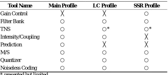
In order to allow a tradeoff among the quality, the memory and processing power requirements, the AAC system offers three profiles: main profile, low-complexity (LC) profile, and scalable sampling rate (SSR) profile.
Main profile: In this configuration the AAC system provides the best audio quality at the given data rate. All AAC tools are applied except for gain control tool. Thus, it requires most computing power and memory usage.
Low-complexity (LC) profile: The prediction tool and gain control tool are not employed and TNS order is limited in this configuration. Comparing to main profile, this reduces processing power and memory requirements.
Scalable sampling rate (SSR) profile: Gain control tool is used only in this configuration. However, the prediction module is excluded and TNS order and bandwidth are limited. SSR profile provides the lowest complexity and a frequency scalable capability.
Table 3.2 describes the tools used by three profiles.
Tool Name Main Profile LC Profile SSR Profile
Gain Control ╳ ╳ ○ Filter Bank ○ ○ ○ TNS ○ ○* ○* Intensity/Coupling ○ ○ ╳ Prediction ○ ╳ ╳ M/S ○ ○ ○ Quantizer ○ ○ ○ Noiseless Coding ○ ○ ○
Table 3. 2 Tools used by three profiles * presented but limited
3.2 Filter Bank and Block Switching
Filter bank is a fundamental component of MPEG-2 AAC system that transforms the time-domain input signals into a time-frequency representation. This conversion is done by a forward modified discrete cosine transform (MDCT) in the encoder.
3.2.1 MDCT
The modified discrete cosine transform (MDCT) is a Fourier-related transform based on the type-IV discrete cosine transform (DCT-IV), with the additional property of being lapped. This overlapping, in addition to the energy-compaction quality of the DCT, makes the MDCT especially attractive for signal compression applications, since it helps to avoid artifacts stemming from the block boundaries.
In AAC system, the filterbank takes the appropriate block of input samples, modulates them by an appropriate window function, and performs the MDCT. Each block of input samples is overlapped by 50% with the immediately preceding block and the following block.
The expression for the MDCT is
∑
− = + + = 1 0 0 )] 2 1 )( ( 2 cos[ ) ( 2 ) ( N n in i n n k N n x k X π , for 2 0 ≤ k < N , (3.1) where inx = windowed input sequence,
n = sample index,
k = spectral coefficient index, i = block index,
N = window length of the one transform window based on the window_sequence value, 0
3.2.2 Window Shape
The frequency selectivity of an MDCT filter bank is dependent on the window function. A window function commonly used in audio coding is the sine window. This window produces a filter bank with good separation of nearby spectral components. Another window function provided in AAC system is the Kaiser-Bessel derived (KBD) window which allows optimization of the transition bandwidth and the ultimate rejection of the filter bank.
Sine window coefficients are given as follows:
))
2
1
(
sin(
)
(
, _=
n
+
N
n
W
SIN LEFT Nπ
2
0
n
N
for
≤
<
(3.2)))
2
1
(
sin(
)
(
, _=
n
+
N
n
W
SIN RIGHT Nπ
for
N
≤
n
<
N
2
(3.3)Kaiser-Bessel derived window coefficients are given as follows:
∑
∑
= ==
2 0 0 , _)]
,
(
'
[
)]
,
(
'
[
)
(
N p n p N LEFT KBDp
W
n
W
n
W
α
α
2
0
n
N
for
≤
<
(3.4)∑
∑
= − ==
2 0 0 , _)]
,
(
'
[
)]
,
(
'
[
)
(
N p n N p N RIGHT KBDp
W
n
W
n
W
α
α
for
N
≤
n
<
N
2
(3.5) where 'W , Kaiser-Bessel kernel window function is defined as follows:
[ ]
πα πα α 0 2 0 4 4 0 . 1 ) , ( ' I N N n I n W ⎥ ⎥ ⎥ ⎦ ⎤ ⎢ ⎢ ⎢ ⎣ ⎡ ⎟⎟ ⎟ ⎠ ⎞ ⎜⎜ ⎜ ⎝ ⎛ − − = 2 0 n N for ≤ ≤ (3.6)[ ]
2 0 0 ! 2∑
∞ = ⎥ ⎥ ⎥ ⎥ ⎥ ⎦ ⎤ ⎢ ⎢ ⎢ ⎢ ⎢ ⎣ ⎡ ⎟ ⎠ ⎞ ⎜ ⎝ ⎛ = k k k x x I (3.7)α = kernel window alpha factor, ⎪⎩ ⎪ ⎨ ⎧ = = = 256 , 6 2048 , 4 N for N for α
The AAC system allows seamless switching between KBD and sine windows. Perfect reconstruction is preserved in the filter bank during window shape changes. Fig. 3.3 shows the window shape switching process. The sequence of windows labeled A-B-C employs the KBD window, whereas the sequence D-E-F shows the transition to and from a single frame employing the sine window.
3.2.3 Block Switching
To adapt the time-frequency resolution of the filter bank to the characteristics of the input signal, AAC system provides two kinds of transformation lengths: the long transformation with 2048 samples is termed a “long” sequence, while the short transformation occur in groups called “short” sequence. The short sequence is composed of eight short block transforms, and each with 256 samples.
This block switching, however, potentially creates a problem of block synchrony between the different channels being coded. To maintain block alignment and to preserve the time-domain aliasing cancellation properties of MDCT and IMDCT, a “start” and “stop” bridge window is used during transitions. Fig. 3.4 shows the window overlap-add process appropriate for both steady-state and transient conditions[1].
According to the window_sequence and window_shape element, different transformation windows are used. All possible combinations are described as follows:
Let N = window length, we have:
⎪ ⎪ ⎩ ⎪ ⎪ ⎨ ⎧ = = = = 2048 , _ _ 2048 , _ _ 2048 , _ _ 2048 , _ _ _ N SEQUENCE STOP LONG N SEQUENCE SHORT EIGHT N SEQUENCE START LONG N SEQUENCE LONG ONLY sequence window ⎩ ⎨ ⎧ window ine s window KBD shape window _ a) ONLY_LONG_SEQUENCE window_shape = = KBD window ⎩ ⎨ ⎧ < ≤ < ≤ = 2048 1024 ), ( 1024 0 ), ( ) ( 2048 , _ 2048 , n for n W n for n W n W RIGHT KBD LEFT
window_shape = = sine window
⎩ ⎨ ⎧ < ≤ < ≤ = 2048 1024 ), ( 1024 0 ), ( ) ( 2048 , _ 2048 , n for n W n for n W n W RIGHT SIN LEFT b) LONG_START_SEQUENCE window_shape = = KBD window ⎪ ⎪ ⎩ ⎪ ⎪ ⎨ ⎧ < ≤ < ≤ − + < ≤ < ≤ = 2048 1600 , 0 . 0 1600 1472 ), 1472 128 ( 1472 1024 , 0 . 1 1024 0 ), ( ) ( 256 , _ 2048 , n for n for n W n for n for n W n W RIGHT KBD LEFT
⎪ ⎪ ⎩ ⎪ ⎪ ⎨ ⎧ < ≤ < ≤ − + < ≤ < ≤ = 2048 1600 , 0 . 0 1600 1472 ), 1472 128 ( 1472 1024 , 0 . 1 1024 0 ), ( ) ( 256 , _ 2048 , n for n for n W n for n for n W n W RIGHT SIN LEFT c) EIGHT_SHORT_SEQUENCE
The total length of the window_sequence together with leading and following zeros is 2048-bit. Each of the eight short blocks are windowed separately first. The short block number is indexed with the variable j = 0,1,…,7.
window_shape = = KBD window ⎩ ⎨ ⎧ < ≤ < ≤ = 256 128 ), ( 128 0 ), ( ) ( 256 , _ 256 , 0 n for n W n for n W n W RIGHT KBD LEFT ⎩ ⎨ ⎧ < ≤ < ≤ = − 256 128 ), ( 128 0 ), ( ) ( 256 , _ 256 , _ 7 1 n for n W n for n W n W RIGHT KBD LEFT KBD
window_shape = = sine window ⎩ ⎨ ⎧ < ≤ < ≤ = 256 128 ), ( 128 0 ), ( ) ( 256 , _ 256 , 0 n for n W n for n W n W RIGHT SIN LEFT ⎩ ⎨ ⎧ < ≤ < ≤ = − 256 128 ), ( 128 0 ), ( ) ( 256 , _ 256 , _ 7 1 n for n W n for n W n W RIGHT SIN LEFT SIN d) LONG_STOP_SEQUENCE window_shape = = KBD window
⎪ ⎪ ⎩ ⎪ ⎪ ⎨ ⎧ < ≤ < ≤ < ≤ − < ≤ = 2048 1024 ), ( 1024 576 , 0 . 1 576 448 ), 448 ( 448 0 , 0 . 0 ) ( 2048 , _ 256 , n for n W n for n for n W n for n W RIGHT KBD LEFT
window_shape = = sine window ⎪ ⎪ ⎩ ⎪ ⎪ ⎨ ⎧ < ≤ < ≤ < ≤ − < ≤ = 2048 1024 ), ( 1024 576 , 0 . 1 576 448 ), 448 ( 448 0 , 0 . 0 ) ( 2048 , _ 256 , n for n W n for n for n W n for n W RIGHT KBD LEFT
3.3 Temporal Noise Shaping
The handling of transient and pitched input signal has always been a challenge of today’s audio coding, which is due to the so called “pre-echo” phenomenon.
3.3.1 Pre-echo Phenomenon
In psychoacoustic model, we exploit the perceptual effect of simultaneous masking (see Chapter 2). However, from Fig. 2.4, we observed that pre-masking, in the order of 2-5 ms, is much shorter than post-masking. At the same time, to achieve perceptually transparent coding quality, quantization noise must not exceed the time-dependent masking threshold.
This requirement is not easy to meet for perceptual coders. Because quantizing and coding in frequency domain implies that the quantization error introduced in this domain will be spread out in time domain after reconstruction. Assuming sampling rate is 44.1 kHz, AAC system performs 2048-point MDCT which means the
quantization noise can be spread out over a period of more than 46 ms. In particular, if quantization noise is spread out before the onsets of the signal and in extreme cases may even exceed the original signal in level during certain time. Fig. 3.5 gives a pre-echo phenomenon example.
Fig. 3. 5 Pre-echo phenomenon example[39]
Some traditional techniques have been proposed to avoid pre-echo phenomenon, including bit reservoir, gain control and adaptive window switching. Here, AAC provides a new powerful tool called temporal noise shaping (TNS) to further exercise control over the temporal fine structure of the quantization noise even within a filter bank window.
3.3.2 TNS Processing
The basic concept of TNS can be outlined as follows:
Time-frequency duality considerations:
It is well known that signals with an “unflat” spectrum can be coded efficiently either by directly coding spectral values or by applying predictive coding methods to the time domain signal [3]. According to duality between frequency and time domain, we can say that signals with an “unflat” time structure, that is, transient signals can be coded efficiently either by directly coding time-domain signals or by applying predictive coding methods to the spectral values. Table 3.3 summarizes this concept.
Input Signal Optimum Coding
Time Domain Freq. Domain Direct Coding Predictive Coding
Coding of spectral data
Prediction in time domain
Coding of time domain data
Prediction in frequency domain
Table 3. 3 Optimum Coding Methods for Extreme Input Signal Characteristics [4]
Noise shaping by predictive coding:
Although both open-loop and close-loop predictive coding techniques can be employed to provide coding gain, the distribution of quantization error in the final decoded signal are different. If a close-loop prediction scheme is used the error
introduced in the final decoded signal has a “flat” power spectral density (PSD). However, if an open-loop prediction scheme is used, the PSD of its quantization error is known to adapt to the PSD of the input signal. This effectively puts the quantization noise under the actual signal and therefore avoids problems of temporal masking in either transient or pitched signals. Fig. 3.6 shows this concept of DPCM coding. For more details, please refer to [3].
Fig. 3. 6 Comparisons of input (solid) and coding noise (dashed) spectrum [3]
This type of linear prediction coding of spectral data is referred to as the TNS method.
3.4 M/S Stereo Coding
AAC system includes two techniques for stereo coding of signals – mid/side (M/S) stereo coding (also known as sum-difference coding) and intensity stereo coding. Both stereo coding strategies can be combined by applying them to different
frequency regions.
Middle/Side (M/S) stereo coding primarily has two effects: one is to control the imaging of coding noise, as compared to the imaging of the original signal. In particular, this technique is capable of addressing the issue of binaural masking level difference (BMLD). The other is simply to reduce interchannel redundancies.
3.4.1 Binaural Masking Level Difference
The masking threshold of a signal can sometimes be markedly lower down when listening by two ears than when listening by only one. Considering the situation shown in Fig. 3.7(a). White noise from the same noise generator is fed into both ears via headphones. Pure tones, also from the same signal generator, are fed separately into each ear and mixed with the noise. Thus the total signals in two ears are identical. Assuming that the level of the tone is adjusted until it is masked by the noise, i.e. it is at its masking threshold, and let this level be L0 dB. Now that we invert the tone signal at only one ear, i.e. the phase of the tone signal is shifted by 180°, as shown in Fig. 3.7(b). The result is that the tone becomes audible again. The tone can be adjusted to a new level, Lπ, and it is again its masking threshold. The difference
between the two levels, L0 - Lπ (dB), is known as a binaural masking level
Fig. 3. 7 Illustration of the situation in which BMLD occurs [8]
BMLD value may be as large as 15 dB at low frequencies (around 500 Hz), decreasing to 2 dB for frequencies above 1500 Hz.
This phenomenon is not limited to pure tones. Similar effects have been observed for complex tones, transient and pitched signals. Our ability to detect and identify the signals depends on the phase of the signal and noise presented (or lack of correlation in the case of noise).
3.4.2 M/S Stereo Threshold
Due to the BMLD phenomenon stated previously, to prevent stereo unmasking, M and S, left and right thresholds are again calculated:
(
)
(
)
(
)
(
)
⎟⎠⎞ ⎜ ⎝ ⎛ ⎟ ⎠ ⎞ ⎜ ⎝ ⎛ × = ⎟ ⎠ ⎞ ⎜ ⎝ ⎛ ⎟ ⎠ ⎞ ⎜ ⎝ ⎛ × = = ⎟ ⎠ ⎞ ⎜ ⎝ ⎛ × × = ⎟ ⎠ ⎞ ⎜ ⎝ ⎛ ⎟ ⎠ ⎞ ⎜ ⎝ ⎛ × × = = > = − Mengy b Mthr Sthr t Sthr Sengy b Sthr Mthr t Mthr Rthr Lthr t Lengy b Lthr t Lthr Lfthr engy R b Rthr t Rthr Rfthr t t t if Sthr Mthr t max , min , max , min max , min , max , min , min max , min , max max , min , max ) 1 ( / 1 where,Mthr, Sthr, Rthr, Lthr are thresholds of M, S, right and left channel. Mengy, Sengy, Rengy, Lengy are spread energy of M, S, R, L channel. Mfthr, Sfthr, Rfthr, Lfthr are final thresholds
bmax represents BMLD protection ratio, as can be calculated from
( ) ⎥ ⎦ ⎤ ⎢ ⎣ ⎡ ⎟ ⎠ ⎞ ⎜ ⎝ ⎛ + − = 15.5 5 . 15 ), ( min cos 5 . 0 5 . 0 3 10 ) max( b bval b b π (3.8)
where, bval(b): median bark value of bth partition.
3.4.3 L/R and M/S Switching
If the difference between THRl and THRr is less than 2 dB, and the bits required is fewer than L/R mode, the coder will switch to M/S mode, i.e. the left signal for that given band of frequencies is replaced by
2 R L
M = + and the right signal is replaced
by
2 R L S = − .
3.5 Intensity Stereo Coding
Intensity stereo coding exploits the fact that the human perception of high frequencies components relies on the analysis of the energy–time envelopes [7][8] to increase the reduction of irrelevancy at high frequencies. This is done based on the channel-pair concept as used for M/S stereo, the following explanation will use L/R pair for convenience. Instead of transmitting both left and right channel signals, a single representing signal plus directional information will be transmitted only. Thus, the reconstructed signals for the left and right channel consist of differently scaled versions of the same transmitted signals which have different amplitudes but have the same phase information. The energy-time envelope is preserved by means of the scaling operation; however, due to the loss of phase information, the waveform of the original signal is generally not preserved. The directional information, is_position, is computed as: ⎟ ⎟ ⎠ ⎞ ⎜ ⎜ ⎝ ⎛ ⎟⎟ ⎠ ⎞ ⎜⎜ ⎝ ⎛ × = ] [ ] [ log 2 ] [ _ 2 sfb E sfb E NINT sfb position is r l (3.9)
scalefactor bands (see section 3.6.2) by adding spectral samples from the left and right channel (specl[i] and specr[i]) and rescaling the resulting values like
] [ ] [ ]) [ ] [ ( ] [ sfb E sfb E i spec i spec i spec s l r l i = + × (3.10) where
sfb is the index of scalefactor band, NINT means “nearest integer”,
El, Er, Es represent the energy of left, right and sum channel. The sum channel is calculated by summing the squared spectral coefficients.
The signal flow of an intensity stereo coding / decoding scheme is shown in the Fig. 3.9.
Fig. 3. 9 signal flow of an intensity stereo coding / decoding scheme [14]
3.6 Prediction
Prediction is used for an improved redundancy reduction and is especially effective if the signal is more or less stationary. Since a window sequence of type EIGHT_SHORT_SEQUENCE indicates signal changes, i.e. non-stationary signal
characteristics, prediction is used only for long window. There is one corresponding predictor for each spectral component, resulting in a bank of predictors.
3.6.1 Predictor Structure
Backward-adaptive predictors are adopted in AAC system. The predictor coefficients are calculated from preceding quantized spectral components in the encoder as well as in the decoder. Thus, no additional side information is needed for the transmission of predictor coefficients. A second-order backward-adaptive lattice structure predictor is used for each spectral component, so that each predictor is working on the spectral component values of the two preceding frames.
Due to the realization in a lattice structure, the predictor contains two basic elements that are cascaded. The overall estimate results in
) ( ) ( ) (n x ,1 n x ,2 n
xest = est + est (3.11)
In each element, the part xest,m(n),m=1,2 , of the estimate is calculated according to: ) 1 ( ) ( ) ( 1 , n =b×k n ×a×r − n− xestm m m (3.12)
where backward prediction error at stage m, rm(n), is calculated as: ) ( ) ( ) 1 ( ) (n r 1 n b k n e 1 n rm = m− − − × m × m− (3.13) and forward prediction error at stage m, em(n):
) ( ) ( ) (n e n x n e = − − (3.14)
The attenuation factors, a and b are chosen as a = b = 0.953125.
And a least-mean-square (LMS) approach is used here, the prediction coefficients, m
k , are calculated as follows:
(
)
[
]
( ) ) ( ) 1 ( ) ( 2 1 ) 1 ( ) ( 1 2 1 2 1 2 1 2 1 n VAR n COR i i i i n k m m m m n i i n m n i m i n mr
e
r
e
= − + − = + − − = − − = − −∑
∑
α
α
(3.15) with ) ( ) 1 ( ) 1 ( ) (n COR n r 1 n e 1 n CORm =α
× m − + m− − × m− (3.16)[
( 1) ( )]
2 1 ) 1 ( ) ( 2 1 2 1 n e n r n VAR n VARm =α
× m − + m− − + m− (3.17) whereα
is an adaptation time constant which determines the influence of the current sample on the estimate of the expected values. The value ofα
is chosen to be 0.90625.More explanations can be found in [9][10]. Fig. 3.10 shows the second-order backward-prediction lattice structure.
3.6.2 Predictor Control
A predictor control is required to guarantee that there is a prediction gain. The decision, whether the predictor is on or off, is made in the unit of one scalefactor band (see Section 3.6.2). Two considerations are taken into account - First, if prediction gives a prediction gain in that scalefactor band, and all predictors belonged switch on or off accordingly. Second, whether the overall coding gain of current frame compensates at least the additional bits needed for the prediction side information. Prediction is activated only if the above two conditions are met. In order to increase the stability of the predictors, a cyclic reset mechanism is applied, in which all predictors are initialized in a certain time interval. The whole set of predictors are subdivided, in an interleaving way, into 30 so-called reset groups.
Reset Group Number Predictors of Reset Group 1 P0, P30, P60, P90, …. 2 P1, P31, P61, P91, …. 3 P2, P32, P62, P92, ….
…. …. 30 P29, P59, P89, P119, …
Table 3. 4 Reset groups of predictors [2]
Fig. 3.11 shows the block diagram of the prediction unit for one single predictor of the predictor bank. P – predictor ; Q – quantizer ; REC – reconstruction of last quantized value. For more detailed description of the principles can be found in [11].
Fig. 3. 11 Block diagram of prediction unit for one scale factor band [2]
3.7 Quantization
The primary goal of quantization is to quantize spectral data in such a way that the quantization noise fulfills the demands of the psychoacoustic model, and at the same time, the bits required must also be below a certain limit, normally the average number of bits available for a block of audio data.
3.7.1 Nonuniform Quantization Function
The nonuniform quantizer used in AAC is shown as follow:
⎪⎭ ⎪ ⎬ ⎫ ⎪⎩ ⎪ ⎨ ⎧ − ⎥ ⎦ ⎤ ⎢ ⎣ ⎡ = − MAGIC NUMBER i xr quant x r scalefacto common r scalefacto _ 2 ) ( int _ 75 . 0 4 _ (3.18)
Section 3.6.2.
The main advantage of nonuniform quantizer is the implicit noise shaping depending on the coefficient amplitudes. Its increasing signal-to-error ratio (SNR) with rising signal energy is much lower than that in a linear quantizer.
3.7.2 Scalefactor Band
Noise shaping in quantization process is done by using scalefactors. For this purpose, spectrum is divided into several (depending on sampling rates) scalefactor bands which is very similar to the critical bands of human auditory system. Each scalefactor band has a scalefactor that represents a certain gain value. All spectral coefficients belong to that scalefactor band will be rescaled by their scalefactor. The noise shaping is therefore achieved because amplified coefficients have larger amplitudes, and thus obtained a higher SNR after quantization.
3.7.3 Iteration Process
Optimum quantization is done by an iteration process consisting of two nested loops, an inner loop which is aimed at controlling coding bits required and an outer loop which is used to shape the quantization noise. The overall iteration process can be shown as Fig. 3.12.
Fig. 3. 12 A simplified block diagram of iteration process BEGIN
Calculation of number of available bits
Reset of iteration variables
All spectral values zero?
Outer Iteration Loop
Calculate the number of unused bits
RETURN yes
3.7.3.1 Inner Iteration Loop
The task of inner iteration loop is controlling the coding bit required by adjusting quantizer step size until all spectral data can be encoded with the number of available bits. If the number of bits needed for encoding is higher than available bits, the quantizer step size is increased, and the process will repeat until reaching its goal. Thus, inner iteration loop is also called rate control loop. A simplified processing description is as follows:
1. At the beginning, the spectral data are quantized by nonuniform quantization function (3.18).
2. Number of bits required to encode the quantized data is counted.
3. If the number of bits required is higher than the number of available bits, the quantizer step size is increased, and go back to (1), repeating the whole process. 4. Else, the inner iteration loop is ended.
Fig. 3. 13 A simplified block diagram of inner iteration loop
3.7.3.2 Outer Iteration Loop
The task of outer iteration loop is amplifying the scalefactor bands in such a way that the demands of the psychoacoustic model are achieved. Thus, outer iteration loop is also called distortion control loop. A simplified processing description is as follows:
1. At the beginning, no scalefactor is amplified. 2. Inner iteration loop is called.
3. The distortion causes by quantization of every scalefactor band is calculated. BEGIN
Nonlinear quantizer
Noiseless coding (count number of bits used)
Number of bits used less than number of available bits ?
END yes
no Increase quantizer step size
4. The actual distortion is compared with the permitted distortion calculated by psychoacoustic model.
5. If it is the best result so far, store this result, and this process stops. Note that this iteration process is not always converges.
6. Amplifying the scalefactor band which has a higher distortion than the allowed. 7. If all scalefactor bands have been amplified, this process stops.
8. If the distortions of all scalefactor bands are smaller than permitted, this process stops.
9. Otherwise, the whole process will repeat.
BEGIN
Inner Iteration Loop
Calculate distortion in all scalefactor bands
Best result so far?
Amplify sfbs with more than the allowed distortion
RETURN
yes
no
All sfbs amplified?
At least one band with more than the allowed distortion?
END Store best result
Store best result no
no
yes
Fig. 3. 14 A simplified block diagram of outer iteration loop
3.8 Noiseless Coding
Noiseless coding is used to further reduce the redundancy of scalefactors and the quantized spectrum. This is done by lossless packing of quantized spectral data exploiting statistical dependencies and other properties.
3.8.1 Grouping and Interleaving
As for the window sequence of type EIGHT_SHORT_SEQUENCE, there could be a possibility that some of eight short blocks are very different from the other. For example, the first three sets are nearly silent in time domain, the next two sets are actually where the onset event happens, and the final three are the decay of the event. In such cases, sets of 128 coefficients that have similar statistics are grouped together and interleaved to form a single spectrum. Fig. 3.15 shows the grouping example stated above.
indexed as
C[g][w][b][k]
where
g is the index of groups,
w is the index of windows within a group,
b is the index of scalefactor bands within a window, k is the index of coefficients within a scalefactor band.
After interleaving the coefficients are indexed as
C[g][b][w][k]
This has the advantage of combining the high-frequency zero-valued coefficients (due to band-limiting) within each group. Fig. 3.16 shows the spectral order within one group before interleaving, and Fig. 3.17 shows the spectral order after interleaving.
Fig. 3. 16 Spectral order within one group before interleaving
Fig. 3. 17 Spectral order after interleaving
The first step of noiseless coding is a method of dynamic range compression that may be applied to the spectrum. Up to four coefficients can be coded separately as magnitudes in excess of one, with a value of ± 1 left in the quantized coefficient array to carry the sign. The “clipped” coefficients are coded as integer magnitudes and an offset from the base of the coefficient array to mark their location. This method is applied only if it results in a net savings of bits.
3.8.3 Huffman Coding
A variable-length Huffman coding is employed to compensate the nonuniform probability distribution for the levels in quantizer and to represent n-tuples of quantized coefficients. In the AAC system, Huffman codewords are drawn from one of 11 codebooks. The maximum absolute value of the quantized coefficients that can be represented by each Huffman codebook and the number of coefficients in each n-tuple for each codebook is shown in Table 3.4. There are two codebooks for each maximum absolute value, with each representing a distinct probability distribution. The best fit is always chosen.
Codebook Index n-Tuple Size Maximum Absolute Value Signed
0 0 1 4 1 Yes 2 4 1 Yes 3 4 2 No 4 4 2 No 5 2 4 Yes 6 2 4 Yes 7 2 7 No 8 2 7 No
10 2 12 No
11 2 16(ESC) No
Note that codebook 0 indicates all coefficients within that scalefactor band are zero, and codebook 11 can especially represent those who have an absolute value greater than or equal to 16, and a special escape coding mechanism is used to represent them. For each coefficient magnitude greater or equal to 16, an escape sequence is appended, as follows:
escape sequence = <escape_prefix><escape_separator><escape_word>
where
<escape_prefix> is a sequence of N binary “1’s”, <escape_separator> is a binary “0”,
<escape_word> is an N+4 bit unsigned integer, MSB first and N is a count that is just large enough so that the magnitude of the quantized coefficient is equal to
> < + + word escape N _
2
( 4) .3.8.4 Sectioning
The noiseless coding segments the scalefactor bands into sections. Each section uses only one Huffman codebook, thus the number of bits needed to represent the full block is minimized.
Section is dynamic and typically varies block from block. This is done using a greedy merge algorithm by starting with the maximum possible number of sections (only one scalefactor band per section). Sections are merged if the resulting merged section needs lesser number of bits. If the sections to be merged use different Huffman codebooks, the codebook with higher index is always chosen.
3.9 Gain Control
The gain control module is employed only in the SSR profile. It consists of a polyphase quadrature filter (PQF), gain detectors, and gain modifiers. By neglecting the signals from the upper bands of PQF, this output bandwidths can be 18, 12, and 6 kHz when one, two, or three PQF outputs are ignored, respectively.
The advantage of this scalability is that the complexity can be reduced as the output bandwidth is reduced.
3.9.1 Polyphase Quadrature Filter
The PQF splits each audio channel’s input signal into four frequency bands of equal width. The coefficients of each band’s PQF are given by
3 0 , 95 0 ), ( 16 ) 5 2 )( 1 2 ( cos 4 1 ≤ ≤ ≤ ≤ ⎥⎦ ⎤ ⎢⎣ ⎡ + + = i n Q n n i hi π (3.19) Where, 95 48 ), 95 ( ) (n = Q − n ≤ n ≤ Q
The Q(n) is the filter coefficients that are standardized in [2].
3.9.2 Gain Detector
indicating the location and level of gain modification for each segment. Note that the gain detector has a one-frame delay.
3.9.3 Gain Modifier
The gain modifier applies gain control to the signal in each PQF band by windowing the signals of the gain control function. Fig. 3.18 shows the block diagram of gain control module.
Fig. 3. 18 Block Diagram of AAC encoder gain control module [2]
3.10 Bitstream Format
Audio Data Interchange Format (ADIF): The audio bitstream contains one single header with all information necessary to control the decoder. The main application of ADIF is exchange of audio files.
ADIF block block block block block
Audio Data Transport Stream (ADTS): The audio bitstream consists of a sequence of frames with headers similar to MPEG-1 audio frame headers. The encoded audio data of one frame is always contained between two sync words.
ADTS block ADTS block ADTS block
There are mainly five elements in the bitstream: audio data element, data stream element (DSE), program configuration element (PCE), fill element (FIL), and terminator (TERM). Audio data element also consists of four possible elements: single channel element (SCE), channel pair element (CPE), coupling channel element (CCE), and low frequency enhancement channel element (LFE).
SCE contains coded data for a single audio channel. CPE contains data for a pair of channels, and the two channels may share common side information. CCE represents the information for intensity stereo coding. LFE gives the low frequency (under 120 Hz) audio data. PCE contains program configuration data, such as profile, sampling rate, channel information, etc. FIL is used when transporting over a constant rate channel to adjust instantaneous bitrate. DSE contains any additional data that is not part of the audio information itself. TERM indicates the end of a raw data block. Example of possible bitstreams are:
The syntax of a single channel element (SCE)
Mono signal
Stereo signal
5.1 channel signal
If the bitstreams are to transmit over a constant rate channel
If the bitstreams are to carry ancillary data and run over a constant rate channel
CHAPTER 4. MPEG-2/4 LC AAC Encoder
Optimization
Comparing with main profile, low complexity (LC) profile significantly reduces memory usage and computational effort, but still maintains good quality [1]. Therefore, we choose low complexity profile to implement and this is also the most commonly used profile.
4.1 Complexity Analysis
Table 4.1 shows the computational demand of a standard AAC LC implementation from MPEG reference coder:
Module Percentage Psychoacoustic Model 22%
Filter Bank 5%
Quantization 64% Others 9% Table 4. 1 Distribution of resources in AAC-LC encoder [21]
The most demanding module is quantization due to the presence of nested loops. Psychoacoustic model also takes up to 22% computation effort. Besides these two
4.2 Removal of Block Switching
Modern audio compression algorithm often adopts dynamic block switching to avoid pre-echoes (see Section 3.3.1). In general, psychoacoustic model decides whether block type changes or not depending on perceptual entropy. However, the calculation of perceptual entropy requires lots of computation effort.
A related research [22] shows that encoding without block switching didn’t cause significant negative effect, TNS module in AAC system also aims at controlling pre-echo phenomenon which can compensate the lack of block switching. Under these considerations, we remove the mechanism of block switching. For this, not only the calculation of perceptual entropy, but also the complexity of block synchrony and short block related grouping and interleaving algorithm are eliminated.
4.3 Fast MDCT
AAC uses MDCT with 50% overlap in its filterbank module. However, there are lots of multiply-accumulation operation within this module, thus adopting a fast algorithm is necessary. According to [20], MDCT can be rewritten as the real part of odd-time odd-frequency discrete Fourier transform (O2DFT), and finally need only N/4-point FFT calculation:
Coefficient number k of O2DFT of length N is defined as:
( )( )
∑
− = + + − = = 1 0 1 2 1 2 2 ] [ 2 } { N r r k N j r k N u U u e DFT O k π (4.1){
}
( )( ) ⎭ ⎬ ⎫ ⎩ ⎨ ⎧ − = =∑
− = + + − 1 0 1 2 1 2 2 2 ) 4 / ( Re ) ( Re ) ( N r r k N j e N r x k DFT O k X π (4.2)[26][20] further presented a fast algorithm for calculating:
(
)
(
)
{
odd xr N}
X( )
k DFT O W = 2 − /4 = (4.3) as{ }
{ }
} Im{ } Re{ Im Re 2 1 2 2 1 2 2 2 k k N k k N k k N k k P W P W P W P W − = − = = = − − − − + (4.4) Where k N k k U jU P 2 2 2 − + = ( )( )∑
− = + + − + − = /41 0 2 2 2 2 2 / 2 2 1 2 1 ) ( 2 N r r k N j r N r ju e u π (4.5) ( ) ( ) 4 4 4 4 4 3 4 4 4 4 4 2 1 FFT po N N r rk N j r N j r k N j e e u e int 4 1 4 / 0 4 / 2 2 2 ) ' ( 2 8 1 8 1∑
− = − + − + − ⎥ ⎦ ⎤ ⎢ ⎣ ⎡ = π π π r N r r u ju u ' /2 2 * = − + (4.6)Through this process introduced in [26][20], only even indices are calculated because of the basic symmetries of the O2DFT. Another saving of 50% computation is calculating two values simultaneously, as shown in (4.5). Finally, only one N/4 point
4.4 Simplified TNS
In general, TNS method is the linear prediction performed in frequency domain. We use the popular Levinson-Durbin recursive procedure to achieve linear predictive coding (LPC). The TNS prediction order of LC profile is designed to be 12 as described in [2]. Fig. 4.1 shows the basic TNS implementation flow:
Fig. 4. 1 Original TNS implementation flow
We are curious about how often TNS is active, therefore, the percentage of whether TNS is finally applied is statistically measured. Table 4.2 shows the result.
TNS filtered data (ON), or the same as input data (OFF)
N
12th-order Levinson-Durbin Recursion
TNS Filter Set up prediction 12th-order Autocorrelation
Y
Gain > TNS Threshold ? ON OFF Input data coefficients Gain ComputationTest audio sample Active percentage
Violoncello[23] 5.5% Quartet[23] 19.9% Soprano[23] 6.7%
Radio[24] 4.3% Table 4. 2 the percentage of TNS being active
We found that the active percentage is pretty low, however, the prediction gain has to be computed every time no matter TNS is finally on or off. Generally, the procedure to obtain prediction gain (including autocorrelation and Levinson-Durbin recursion blocks) requires as much computing effort as TNS filter, see Table 4.3. If further taking the active frequency into account, prediction gain computation actually contributes the most complexity in TNS module. Thus, if we can decide whether TNS is on or off earlier, that is, before 12th-order LPC has been completed, the complexity will be reduced.
Block Percentage Gain Computation 49.5%
TNS Filter 49.5%
Others 1% Table 4. 3 Distribution of resources in TNS module (TNS is finally “ON” case)
To eliminate this over computation, we propose using 6th order prediction gain to determine if LPC procedure will go on. Fig. 4.2 shows the modified TNS implementation flow.
Fig. 4. 2 Modified TNS implementation flow
The matching percentage of this early-deciding mechanism is about 90% in average. Table 4.4 shows some results.
TNS Filter Set up prediction
TNS filtered data (ON), or the same as input data (OFF) 6th-order Levinson-Durbin Recursion
6th-order Autocorrelation
N
Y
Gain > TNS Threshold ? ON OFF Input data Gain > 6th_order_TNS_Threshold ?7~12th-order Levinson-Durbin Recursion 7~12th-order Autocorrelation
![Fig. 2. 1 The absolute threshold of hearing [17]](https://thumb-ap.123doks.com/thumbv2/9libinfo/7682532.142376/15.892.274.654.124.418/fig-absolute-threshold-hearing.webp)
![Table 2. 1 Critical bands. F c – center frequency of the critical band [16]](https://thumb-ap.123doks.com/thumbv2/9libinfo/7682532.142376/16.892.174.740.176.1046/table-critical-bands-f-center-frequency-critical-band.webp)
![Fig. 2. 4 Schematic representation of temporal masking effect [16]](https://thumb-ap.123doks.com/thumbv2/9libinfo/7682532.142376/18.892.143.755.511.715/fig-schematic-representation-temporal-masking-effect.webp)
![Fig. 3. 3 Example of window shape switching process [1]](https://thumb-ap.123doks.com/thumbv2/9libinfo/7682532.142376/28.892.152.681.591.1083/fig-example-window-shape-switching-process.webp)
![Table 3. 3 Optimum Coding Methods for Extreme Input Signal Characteristics [4]](https://thumb-ap.123doks.com/thumbv2/9libinfo/7682532.142376/34.892.135.758.559.860/table-optimum-coding-methods-extreme-input-signal-characteristics.webp)
![Fig. 3. 7 Illustration of the situation in which BMLD occurs [8]](https://thumb-ap.123doks.com/thumbv2/9libinfo/7682532.142376/37.892.268.653.116.392/fig-illustration-situation-bmld-occurs.webp)
![Fig. 3. 9 signal flow of an intensity stereo coding / decoding scheme [14]](https://thumb-ap.123doks.com/thumbv2/9libinfo/7682532.142376/40.892.208.713.549.855/fig-signal-flow-intensity-stereo-coding-decoding-scheme.webp)
![Fig. 3. 10 The second-order backward-prediction lattice structure [1]](https://thumb-ap.123doks.com/thumbv2/9libinfo/7682532.142376/42.892.144.766.299.722/fig-second-order-backward-prediction-lattice-structure.webp)
![Table 3. 4 Reset groups of predictors [2]](https://thumb-ap.123doks.com/thumbv2/9libinfo/7682532.142376/43.892.171.715.555.795/table-reset-groups-predictors.webp)
