打預防針或提前引爆？盈餘預測，監理及風險傾向

(1)

科技部補助專題研究計畫成果報告

期末報告

N 打預防針或提前引爆？盈餘預測，監理及風險傾向

計畫類別：個別型計畫計畫編號： MOST 102-2410-H-004-054- 執行期間： 102 年 08 月 01 日至 103 年 09 月 30 日執行單位：國立政治大學經濟學系計畫主持人：何靜嫺計畫參與人員：碩士班研究生-兼任助理人員：陳年億博士班研究生-兼任助理人員：傅中原博士班研究生-兼任助理人員：傅中原處理方式： 1.公開資訊：本計畫涉及專利或其他智慧財產權，2 年後可公開查詢 2.「本研究」是否已有嚴重損及公共利益之發現：否 3.「本報告」是否建議提供政府單位施政參考：否

中華民國 103 年 12 月 25 日

(2)

中文摘要：大多數文獻研究經理人提供盈餘預測的誘因及動機. 且多數專注於分析經理人盈餘預測的資訊性及短期股價效果. 本文的重心在於經理人盈餘預測所造成的長期效果, 及是如何的所有權及薪資結構促使經理人提供造成不同長期效果的預測. 本計畫可望將盈餘預測的長期效果與所有權及薪資結構相連結, 因此, 預期將可填補不完全資訊模型與公司監理間的關係, 並可導出可供實證的結論來解釋所有權及薪資結構, 與經理人貢獻及盈餘預測的長期效果間的關係. 本文模型將說明所有權及薪資結構是導致經理人提供導致不同長期效果(打預防針或提前引爆)的預測的主因. 換言之, 與其他就行為角度來分析投資人過度或過少反應的文獻不同, 本文主張理性的經理人其實已經預見此長期效果之不同, 而刻意選擇造成不同長期效果的盈餘預測來獲取最高的經理人報償. 中文關鍵詞：盈餘預測, 公司治理, 風險傾向

英文摘要： A large amount of literature examines

managers｀ incentives to provide earnings forecasts. Most studies focus on the informativeness of

management forecasts and their short term reactions on stock prices. Our interest is in the long term impacts of management forecasts, as well as the

compensation structures that motivate the managers to provide the forecasts that cause these different long term reactions. The linkage between compensation structure and the long term impacts of management forecasts will bridge the gap between signaling models and the corporate governance concerns about whether management disclosures are substitutes or complements to corporate governance. It also provides testable results that explain the relation between ownership structure, compensation, managerial effort, and the long term effects on stock prices.

Our model will demonstrate that ownership and compensation structures are the main factors that motivate the managers to provide the forecasts that cause different long term reactions (inoculation or preignition). In other words, in contract to the

(3)

large volume of works on addressing

investors｀ behavioral reasons for over or under reactions, we assert that managers are actually aware of this difference in long term reactions, and they deliberately choose the forecasts that trigger different reactions to exploit the maximal benefit from managerial compensations.

(4)

Preignition or Inoculation? An Interpretation

of Stock Price Trends in Management Forecasts

Shirley J. Ho

National Chengchi University

Email: [email protected]

December 25, 2014

Abstract

A large amount of literature examines managers’ incentives to provide earnings fore-casts. Most studies focus on the informativeness of management forecasts and their short term reactions on stock prices. Our interest is in the long term impacts of management forecasts, as well as the compensation structures that motivate the managers to provide the forecasts that cause these different long term reactions. The linkage between compen-sation structure and the long term impacts of management forecasts will bridge the gap between signaling models and the corporate governance concerns about whether manage-ment disclosures are substitutes or complemanage-ments to corporate governance. It also provides testable results that explain the relation between ownership structure, compensation, man-agerial effort, and the long term effects on stock prices. Our model will demonstrate that ownership and compensation structures are the main factors that motivate the managers to provide the forecasts that cause different long term reactions (inoculation or preigni-tion). In other words, in contract to the large volume of works on addressing investors’ behavioral reasons for over or under reactions, we assert that managers are actually aware of this difference in long term reactions, and they deliberately choose the forecasts that trigger different reactions to exploit the maximal benefit from managerial compensations.

(5)

1 Introduction

A large accounting literature examines managers’ incentives to provide earnings forecasts. Most studies focus on the informativeness of management forecasts and their short-run reactions on stock prices. Some representative papers include Patell (1976), Penman (1980), Waymire (1984), Baginski, et al.(1993), Skinner (1994), Williams (1996), Stocken (2000), Miller (2002), and Hutton, Miller and Skinner (2003).

Our interest is in the long-run impacts of management forecasts, as well as the compensation structure that motivates the managers to provide the forecasts that cause these diﬀerent long run reactions. The linkage between managerial compensation and the long-run impacts of management forecasts will bridge the gap between signaling models and the corporate governance concern about whether management disclosures are subsitutes to corporate gover-nance.1 _{It also provides testable results that explain the relation between ownership structure,}2

compensation, managerial eﬀort, and the long run eﬀects on stock prices.

We consider two specific long-run impacts subsequent to the announcement of management forecasts. The first is the manager’s effort decision in the production stage, which together with the firm’s future prospect will determine the level of actual earnings. Unlike the conventional moral hazard model, managerial effort will determine the true state of private information (i.e., the actual earnings) to be revealed in the signaling process. Hence, upon deciding the informativeness of managerial forecasts, managers also need to choose the effort level to be committed in the production process. We show that both shirking and overworking can happen 1_{See Healy et al. (1999),Bushee and Noe (2000), Core (2001), Bens (2002), Bushman et al. (2004), Fan and}

Wong (2002), Ajinkya et al. (2005) Francis et al. (2005a, 2005b),Karamanou and Vafeas (2005) Ali et al. (2007) and Hope and Thomas (2008).

2_{For example, Frankel, McNichols, and Wilson (1995) conclude that a firm that does not require external}

financing faces less pressure from Wall Street and has fewer concerns with temporary undervaluation, whereas such firms are less likely to provide earnings guidance of any sort (selective or public). Eng and Mak (2003) examine the relation between ownership structure and disclosure in the broader context of voluntary disclosure in the financial statements.

(6)

in equilibrium.

The second impact involves a comparison between the stock price following the release of earnings forecast (denoted as  (_{)), and the price following the publication of actual}

earn-ings (denoted as  ()). We can classify the observations into two groups: inoculation and preignition.3 The definitions for inoculation and preignition vary with the content of firm’s future prospect. That is, if the prospect is good, then inoculation means  (_{) (), while}

preignition means  (_{)  (). On the other hand, if the prospect is bad, then inoculation}

means  (_{)  (), while preignition means  (}_{)  ().}

Our model will demonstrate that ownership and compensation structures are the main fac-tors that motivate the managers to provide the forecasts that cause the different long-run re-actions (inoculation or preignition). In other words, in contract to the large volume of works on addressing investors’ behavioral reasons for over or under reactions (see Kuhnen, 2012), we assert that managers are actually aware of this difference in long-run reactions, and they delib-erately choose the forecasts that trigger different reactions to exploit the maximal benefit from managerial compensations.

To characterize the circumstances that cause the two diﬀerent impacts (inoculation or preig-nition) of management earnings forecasts, we consider a signaling model where a privately in-formed manager issues an earnings forecast to signal his information about the future prospect as well as the precommitted eﬀort level, and public investors will determine stock price based on the public information provided by the manager. The managerial compensation is a weighted sum of stock options and performance bonus, and in the basic model we assume that investors are risk neutral.

As noted by Beyer, et al. (2010), "models that further explore optimal compensation struc-tures and consider their eﬀect on management’s disclosure decisions have the potential to provide new insights into both firms’ disclosure behavior and optimal incentive structures." Moreover, Kanodia (2006) suggests that "models that incorporate disclosure decisions alongside with other 3_Inoculation_{and preignition are defined in terms of stock price, while the concepts of overshooting and}

(7)

(real) decisions or effort allocation allow us to obtain a better understanding about how firms’ disclosure policies affect not only market valuations but also firms’ other (real) decisions and cash flows and the welfare of different shareholder groups."

Our preliminary results are the following. First, the conditions for a full eﬀort truth-telling equilibrium where the forecast truly reveals the actual earnings are when the penalty of mis-reporting is infinite or when the proportion of stock option in the managerial compensation is equal to 2

3 At this level, the benefit from the increase in stock price is oﬀset by the implicit

cost from the decrease in performance bonus. Second, there exist equilibria where the manager shirks and lies more in his management forecasts as well as equilibria where the manager over-works and being more honest in his management forecast. Third, when there is good news, the manager can either increase eﬀort or lie more, while when there is bad news, the manager will either decrease eﬀort or lie less.

Since the future prospect involves good and bad news, we will consider investors with mean-variance utilities, and examine how investors risk attitudes will alter the manager’s eﬀort and disclosure strategy. We then derive the optimal compensation structure and provide the empir-ical analysis.

1.1 Related Literature

Our paper not only bridges the gap between signaling models and the corporate governance concerns of management earnings forecasts, but also provides testable results that explain the relation between ownership structure, compensation, managerial eﬀort, and the long term eﬀects on stock prices (inoculation or preignition).

To characterize the circumstances that cause diﬀerent long term impacts, we consider a signaling model where a privately informed manager issues an earnings forecast to signal his in-formation about the future prospect as well as a precommitted eﬀort level, and public investors will determine stock price based on the public information provided by the manager. Our model is an adaptation from Guttman, Kadan and Kandel (2006) (see also Fischer and Verrecchia,

(8)

2000), who consider the short term reactions of earnings forecasts on stock prices. The manager will maximize stock price, and the main contribution of Guttman, Kadan and Kandel (2006) is to characterize partial revelation equilibria which explains the evidence such as range forecasts (in contrast to the separating equilibria by Riley (1979) and Stein (1989)). Our setup is different in three aspects. First, our model assumes that the managerial compensation is a weighted sum of stock option and performance bonus. The weights on the stock option can be alternatively interpreted as different ownership structures. Thus we are able to characterize the condtions on ownership and compensation structures that motive the manager to provide different earn-ings forecasts. Second, in our model, the actual earnearn-ings are endogenously determined by the manager’s effort decisions. With this framework, we can study the trade-off between corporate governance and management earnings forecast. Third, we consider the long term impacts on management effort and the stock price, both of which are not addressed in their model.

Beyer, et al. (2010) provide a thorough survey for recent works on management earnings forecasts. We repeat the parts that are related to our model, including the pioneering works that use singling models to address management earnings forecasts, the relation with manage-rial compensation, and the trade-oﬀ between corporate governance and management earnings forecasts.

1.1.1 Informativeness

The pioneering works by Grossman and Hart (1980), Grossman (1981), Milgrom (1981) and Milgrom and Roberts (1986) identify conditions under which firms voluntarily disclose all their private information. Later contributions extend this "unravelling result" by considering costly disclosure (e.g., Jovanovic, 1982; Verrecchia, 1983, 1990a; Dye, 1986; Lanen and Verrecchia, 1987), and conclude that information is favorable when it reveals that asset values are expected to be high. This disclosure costs can also include the consequential costs resulting from the proprietary nature of the information (see Verrecchia, 2001; Wagenhofer, 1990; Fischer and Verrecchia, 2004; Arya, et al., 2009).

(9)

a quadratic function of misreproting in earnings forecast, and an implicit cost which describes the negative effect on performance bonus from misreproting. The quadratic cost is assumed so that we have a well defined maximization problem. From this aspect, our model is different from another strand of literature which analyzes the informativeness of management earnings forecasts with cheap talk models (see Crawford and Sobel, 1982; Gigler, 1994; Stocken, 2000). Moreover, as described above, our main difference from the existing literature is to address the influence of ownership structure and managerial compensation on management effort (hence the trade-off with corporate governance) as well as the long term impacts on stock prices.

Our model assumes that after the issuance of earnings forecasts, the managers need to put in eﬀorts which, together with the firm’s future prospect, will determine the level of actual earnings. This is diﬀerent from the line of research which studies the timing of announcing the actual earnings,4 _{profit warnings (Pukthuanthong, 2010) or the conference calls before the}

release of actual earnings (see Bushee, et al., 2003; Kimbrough, 2005), where the actual earnings have already realized.

1.1.2 Compensation

Due to the separation of management and ownership, when shareholders design management’s incentives and the firm’s governance structure in order to maximize the value of their investment, they take into account how incentives and governance structure aﬀect management’s disclosure decisions and hence firm value (John and Ronen, 1990; Core, 2001). However, most models assume that managers attempt to maximize share price (Beyer, et al., 2010), with variants on addressing managers’ incentives to reduce stock prices (Yermack, 1997; Aboody and Kasznik, 2000) or to pursue intertemporal preference on stock prices (Dye, 2010).

Most importantly, Beyer, et al. (2010) note that "models that further explore optimal com-pensation structures and consider their eﬀect on management’s disclosure decisions have the potential to provide new insights into both firms’ disclosure behavior and optimal incentive struc-4_{For example, researches (Yermack, 1997 and Aboody and Kaznik, 2000) show that the timing of corporate}

(10)

tures." Moreover, Kanodia (2006) suggests that "models that incorporate disclosure decisions alongside with other (real) decisions or effort allocation allow us to obtain a better understand-ing about how firms’ disclosure policies affect not only market valuations but also firms’ other (real) decisions and cash flows and the welfare of different shareholder groups."

In our model, the managerial compensation is a weighted sum of stock option and per-formance bonus. With this framework, we can investigate the impacts from ownership and compensation structure on the manager’s disclosure and eﬀort decisions. The optimal compen-sation structure can be derived by calculating the optimal weight to be put on the sock option. Our model will provide a linkage between managerial compensation and the long-run impacts of management forecasts.

Empirically, several studies in this area suggest that voluntary disclosures are related to managerial opportunism. For example, Aboody and Kasznik (2000) find that firms issue bad news earnings forecasts just prior to stock option awards to CEOs. Noe (1999) finds that managers sell more after good news than after bad news disclosures, while Cheng and Lo (2006) find evidence suggesting that firms strategically issue bad news forecasts prior to insider’s net purchases. In a more general setting, Nagar, et al. (2003) argue that equity incentives motivate CEOs to voluntarily issue earnings forecasts.

1.1.3 Market response

Most studies focus on the informativeness of management forecasts and their short-run reactions on stock prices.

Our paper will increase the observation span from the time that earnings forecast are an-nounced till the time after the publication of the actual earnings. We discover an interesting distinction between two long term effects: inoculation and preignition, both of which are defined differently in good or bad news. Our model will characterize the circumstances where managers might change their earnings forecasts for good or bad states,5 _{so that the long term effect would}

5_{Miller and Piotroski (2000) find that managers of firms in turnaround situations are more likely to provide}

(11)

change from inoculation to preignition, or vice versa.

Many researches have studied the market eﬀect of voluntary earnings disclosure for good or bad news. Similar to the distinction between inoculation and preignition, Bernhardt and Campello (2007) find a nonlinear relation between earnings surprises and stock prices as fol-lows. (i) Prices rise less in response to a positive earnings surprise than they fall following a comparably-sized negative earnings surprise; (ii) Greater positive earnings surprises have only marginally positive impacts on returns; but (iii) more negative earnings surprises have sharper adverse impacts on stock price. Researches suggest that the stock market’s asymmetric response to earnings surprises (stock prices respond more to negative earnings surprises than to positive earnings surprises) is particularly large for high-growth firms (Skinner and Sloan 2002). There-fore, managers of firms with higher valuation multiples (price-to-earnings and market-to-book) are likely to face greater pressure not to disappoint (see Matsumoto 2002).

For the diﬀerence between good and bad news, Skinner (1994) and Kasznik and Lev (1995) conclude that managers are more likely to voluntarily preempt bad news than good news, and that bad news disclosures often occur shortly before earnings announcements. Kothari, et al. (2009) find an asymmetric response to good and bad forecast news and conclude that, on average, managers delay the release of bad news (see Dye and Sridhar (1995) and Acharya, et al. (2008)). Contrarily, Aboody and Kasznik (2000) show that firms delay disclosure of good news and accelerate the release of bad news prior to stock option award periods, consistent with managers making disclosure decisions to increase stock-based compensation.

Skinner (1994) find that bad news disclosures generate larger stock price reactions than good news disclosures, and that large negative earnings surprises are preempted more frequently (20-25% of the time) than other earnings releases (preempted less than 10% of the time). Similarly, Skinner and Sloan (2002) find that the market reaction to negative earnings surprises is much stronger than the market reaction to positive earnings surprises. Hutton, et al. (2003) examine the market response to management earnings forecasts and find that bad news earnings forecasts are always informative but that good news forecasts are informative only when supplemented by verifiable forward-looking statements. Hutton and Stocken (2009) use a firm-level measure

(12)

of the accuracy of prior management earnings forecasts and find that the market response to the news in management earnings forecasts increases in the accuracy of prior forecasts.

Finally, there is a strand of literate addressing the impacts on investors’ risk or uncertainty. Our model addresses the reverse impacts by asking whether investors’ risk attitudes (risk averse or risk loving) can change the manager’s disclosure decisions.

Trueman (1986) Dutta and Trueman (2002) consider the reaction on the investors’ uncer-tainty. Morse, Stephan, and Stice (1991) and Baginski, Conrand, and Hassel(1993) indicate that earnings announcements and management forecasts containing a large surprise component can increase the standard derivation across analysts forecasts that constitute the consensus, imply an increase in investor uncertainty. The uncertainty-reducing effects of forecasts with a minimal surprise component. Graham, Harvey and Rajgopal (2005) find that managers make voluntary disclosures to reduce information risk and boost stock price but at the same time, try to avoid setting disclosure precedents that will be difficult to maintain. Suijs (2008) considers an overlapping generations model where investors trade in a firm’s stock. Investment risk is partly determined by the volatility of the stock price at which current investors can sell their shares to the next generation of investors. It is shown that asymmetric reporting of good and bad news is value relevant as it affects the allocation of risk among future generations of shareholders.

2 The Model

Here we present a signaling model with eﬀort decisions to describe how stock price trends (inoculation or preignition) can reveal managers’ private information on firm’s future prospect and their eﬀort decisions. We demonstrate that the choices of inoculation or preignition will depend on the type of information (good or bad news), managerial compensation structures and managers’ cognition bias (overconfidence).

The participants are a privately informed manager and numerously many investors. In a four-stage signaling model, the manager first issues an earnings forecast to signal his information about the firm’s future prospect as well as his choice of eﬀort. The investors calculate the

(13)

expected firm value based on the public information (forecast and actual earnings) and determine the stock price accordingly. Specifically, we consider the following sequence of actions. At  = 1, the manager, who is informed of the firm’s future prospect, issues an earnings forecast. The firm’s future prospect and the manager’s eﬀort level at  = 3 will determine the level of actual earnings to be realized at  = 4 At  = 2, numerous investors observe this forecast, calculate the expected earnings and modify the stock price accordingly. At  = 3, the manager makes his eﬀort decision. The firm’s actual earnings are released and publicized at  = 4 and the public investors observe the actual earnings and modify the stock price accordingly. More details about earnings and the information structure are given as follows.

Incomplete information on prospect and effort The actual earnings are determined by the firm’s future prospect () and managerial effort ( ∈ [0 1]).6 Other inputs such as capital and labor are assumed to be publicly observable, and we use a constant  to summarize the overall impacts from these inputs. Since no private information is contained in , there is no loss of generality to assume that  = 1. Specifically, the actual earnings  are assumed to be a function of firm’s future prospect and effort as follows.

( ) = Φ1−

where 0    1 (1 − ) measures the output elasticity of effort (prospect). The Cobb-Doglous function is assumed because it provides tractable solutions, and it has a property that the effort’s marginal production is increasing with the level of prospect. When the prospect is low, the manager needs to put in more effort to reach the same earnings level as when the prospect is high. This property will reinforce the incentive of the performance bonus in managerial compensation.

We use a parameter Φ ≥ 1 to indicate the manager’s cognitive bias towards the earnings. 6_{Note that managers’ eﬀort decisions are endogenously determined in our model. This is diﬀerent from}

the literature which attributes the CEO-specific characteristic of ability as important factor to determine the likelihood and frequency of issuing a forecast (seeTrueman (1986), Aboody and Kasznik 2000; Nagar, Nanda, and Wysocki 2003; Cheng and Lo 2006).

(14)

When Φ  1 the manager is overconfident about future earnings, and when Φ = 1 the manager is neutral. Next, both the firm’s future prospect and the managerial eﬀort are privately known by the manager. The uninformed public investors believe that  is uniformly distributed over [0 1], and that  is drawn from a normal distribution7 _{with mean  and variance }2_{. The}

cumulative distribution function is  , and the density function is denoted by  . All parameters and the function forms of these distributions are common knowledge.

Public investors will adjust their beliefs, the expected earnings and the stock price according the public information released by the firm. There are two sources of public information: the management forecast (_{) announced at  = 1 and the actual earnings () publicized at  = 4.}

Let  (|₎

and  (|₎

be the posterior cumulative and density functions and (|₎ _be

the expected earnings after observing . Following Guttman, Kadan and Kandel (2006), we assume the following pricing function that maps the set of management forecast into the set of stock price:  :  →  . In particular, the stock price after observing  _is:

 () = (_|) (1)

Numerous investors will dilute any arbitrage benefit and hence the stock price reflects the expected earnings. Waymire (1984) and Ajinkya and Gift (1984) show that there are positive stock price reactions to management forecasts of earnings increases, and negative reactions to forecasts of earnings decreases. When the actual earnings are publicized at  = 4, there is no uncertainty, so  () = 

Manager’s payoﬀ The manager’s payoﬀ  (( ) ₎ _{is the managerial compensation}

minus eﬀort and price manipulation costs. The managerial compensation is a weighted sum of stock option awards and performance bonus, and let 0    1 denote the proportion on stock option awards. Specifically,

 (( ) ) =  µ  () +  (₎ 2 ¶ + (1_{− )}¡_{− (|})¢₋  2 2 −  ((_|₎ − ) 2 2  (2)

(15)

The first two terms represent the managerial compensations, and the last two terms are the eﬀort and manipulation costs. First, since stock price is positively related to stockholders’ returns, we use a weighted sum of  () and  (₎ _{to measure the period-average stock price. Most large}

firms compensate their top executives through stock options, which now represent the largest single component of managerial pay (Murphy, 1999; Kanagaretnam et al., 2004). Baik et al. (2011) conclude that the forecast release will lead to a higher firm value at the end of the period than if the forecast had not been issued, thereby enhancing the manager’s equity-based wealth. Second, a performance bonus is rewarded according to the diﬀerence between actual earn-ings and the expected earnearn-ings. In business practices, a predetermined performance bonus for meeting a specific goal or target is common in the sales industry and for C-suite executives at large companies.8

Third, the eﬀort cost measures the manager’s direct or opportunity cost involved in produc-ing the earnproduc-ings. The manipulation cost represents the manager’s legal, regulatory, or psychic costs, which will be increasing with the forecast dispersion (see Guttman et al., 2006). The quadratic functions of these two cost terms are assumed so that the manager objective function will be concave and the discussion on the manager’s optimization problem is meaningful.

Equilibrium We look for the perfect Bayesian equilibrium of this game, including a dis-closure strategy, an eﬀort decision and the investors’ beliefs updating processes.

Let  : [0 1] ×  →  with (( )) =  _{denote the disclosure strategy which is a}

correspondence that maps the actual earnings to management forecast. When making the announcement of _

the manager needs to pre-commit to an effort level. Let  :  → [0 1] with () =  denote the manager’s effort decision, which is a real function that maps the future prospect to effort level. A perfect Bayesian equilibrium is a pair of strategies ( ) together with investors’ posterior beliefs that satisfy the following conditions.

(i) For all , ((( ) ()) ∈ arg max

_

 (( ) )

(16)

(ii) The posterior beliefs  (|) and (|) are consistent with the disclosure strategy by Bayes’ rule wherever possible.

Notice that although the forecast is announced at  = 1 while the eﬀort decision is made at  = 3, the only new information released at  = 2 is the price change caused by the announce-ment. Since there is no other uncertainty in the updating process, the informed manager faces the same maximization problem at  = 1 and  = 3+

2.1 Characterization of Equilibrium

We now demonstrate how stock price trends are linked with the manager’s disclosure strategy. First, we substitute the pricing function  (_{) = (}

|₎ _{and  () =  into  (( ) }_)

Let 4 = (|₎

−  denote the stock price trend, and we can rewrite the manager’s payoﬀ as a function of  and 4  (( ) ) =  µ  () +  (₎ 2 ¶ + (1_{− )}¡_{− (|})¢_{− }((| ₎ − ) 2 2 −  2 2 = ₋ 2(− (| _{)) + (1} − )¡_{− (|})¢_{− }((| ₎ − ) 2 2 − 2 2 = Φ1−₋ 2 2 +  24 − (1 − )4 −  4 2 2 ≡ (( ) 4) (3)

4 describes the stock price change from the "perceived" earnings ((|_{)) to the actual}

earnings (). We can see the net benefit of increasing 4 and increasing  from equation (3). The benefit of increasing 4 is to the increase of compensation from the stock option awards: 24

The cost of increasing 4 is the loss from performance bonus: −(1 − )4 and the manipulation cost: 4₂2 On the other hand, the net benefit of increasing  is the increase in final earnings minus the eﬀort cost: ₂2.

Hence we can rewrite the manager’s maximization problem as:

max

4  (( )4)

The first order condition of maximization is:9

 (_{4 )}{Φ _1− ₋2 2 +4 µ (3 2 − 1) −  24 ¶ } = 0 (4)

(17)

The manager seeks for a pair of (4 ) to keep this equality satisfied. Although the forecast  _{is announced at  = 1 while the eﬀort decision is made at  = 3, when we transform the}

maximization problem to a choice of 4 the manager needs to pre-commit to an eﬀort level. This pre-committed eﬀort determines an earnings level first, then 4 is added in to become the forecast 

Notice that 4 refers to the stock price change from the "perceived" earnings ((|_{)) to}

the actual earnings (). It is diﬀerent from the "precision of announcement", which is defined as 

−  Also, the two relevant terms "overshooting" and "undershooting", indicating the cases with 

−   0 and 

−   0 should not be confused with the notions of preignition and inoculation. The definitions of preignition and inoculation are defined in terms of the stock price pattern and vary with the type of information. Specifically, preignition means 4  0 for good news, and 4  0 for bad news, while inoculation means 4  0 for good news, and 4  0 for bad news. Take the case of bad news for example. Preignition means to hide this bad news by confusing the investors with a high earnings forecast. This can avoid a sudden depreciation in current stock price, but when the final earnings realize low, the stock price will eventually drop down. Inoculation, on the other hand, means to reveal this bad news by confusing the investors with a exogenously low earnings forecast. This creates a sudden depreciation in current stock price, but when the final earnings realize better than expectation, the stock price will eventually rise up.

We identify two groups of equilibria: the equilibria with full eﬀort and other equilibria involving shirking or overworking. Full eﬀort refers to the case where the partial derivative

 [Φ

_1−₋2

2] = 0; while shirking or overworking refers to the case where the partial

deriv-ative _[Φ1− ₋ ₂2] ≷ 0 All of these cases are possible since the maximization condition (equation (3)) only requires the sum of net benefit of increasing 4 and  be zero. When the net benefit of increasing  is greater, equal and smaller than zero, then the net benefit of increasing 4 needs to be smaller, equal and greater than zero, respectively, to keep the equality in equation (3) satisfied.

(18)

2.1.1 Full eﬀort equilibrium

In this equilibrium, the partial derivative _[Φ1−₋₂2] = 0Let ∗ denote this full eﬀort. In order to satisfy equation (3), we need the partial derivative _4 [₄¡(3₂ _{− 1) −} ₂₄¢] = 0 That is, (3

2 − 1) − 4 = 0 Let 4∗ denote this stock price trend, and

4∗ = 1 (

3

2 − 1) (5)

Hence, given full eﬀort, the condition for a truth-telling equilibrium (i.e., 4∗ _{= 0) is either}

 =_{∞ or  =} 2₃  = _{∞ indicates that there is a severe penalty for misreporting, and  =} 2₃ requires that two thirds of the managerial compensation are stock option awards. When  = 2₃ the benefit from the increase in stock option award is oﬀset by the implicit cost from the decrease in performance bonus (i.e., (3₂ _{− 1) = 0)}

Proposition 1 _{If  = ∞ or  =} 2₃ then there exists a truth-telling equilibrium where  _truly

reveals the actual earnings . However, if 1 (

3

2 − 1) 6= 0 then there will not be any separating

equilibrium.

When 1 (

3

2 − 1) = 0, the net benefit of increasing 4 is zero. When   2

3 the benefit

from the increase in stock option awards is higher than the decrease in performance bonus and manipulation cost, so 4∗ _{ 0} _{When  } 2

3the benefit from the increase in performance bonus

is higher than the implicit loss from the decrease in stock option awards, so 4∗ _{ 0} _{In other}

words, the choice of 4∗ depends on  As  increases, the chance that   2₃ will increase and the chance that   2₃ _{will decrease. So the probability of choosing 4  0 is increasing in } and the possibility of choosing 4  0 is decreasing in 

Prediction 2 _{The possibility of choosing 4  0 is increasing in ; The possibility of choosing} 4  0 is decreasing in 

Put in diﬀerent content of information, our results predict that for good news, the probability of choosing preignition (in this case, 4  0) is decreasing in  and for bad news, the probability of choosing preignition (in this case, 4  0) is increasing in 

(19)

Intuitively, when the stock option awards increase, the net benefit from increasing 4 is more likely to become positive. The net benefit from increasing 4 is a sum of benefit from stock option award, implicit loss in performance bonus, and explicit cost of price manipulation. Hence the probability of choosing 4  0 will increase with the stock option awards. On the other hand, the probability of choosing 4  0 will decrease with the stock option awards. Put in diﬀerent contents of information, our results predict that, for good news, the probability of preignition (in this case, 4  0) will decrease with the proportion of stock option, while for bad news, the probability of preignition (in this case, 4  0) will increase with the proportion of stock option. In other words, we predict that when the proportion of performance bonus increases, the probability of preignition (inoculation) will decrease (increase) for bad news. That is, managers tend to use inoculation in bad times as the share of performance bonus increases.

2.1.2 Other equilibria

In addition to the full eﬀort equilibrium, we now characterize the properties for other equilibria involving shirking or overworking. If the manager shirks (i.e., _(Φ_1− ₋ 2

2)  0) or

overworks (i.e, _(Φ1− ₋ ₂2)  0)10 then we need to have _4 _{4¡(3₂ _{− 1) −}₂₄¢_{}  0} and  0 to satisfy the first order condition in equation (3).

Information Type and Choices of _{4 and  Here we examine how good news and bad} news affect the manager’s effort and reporting decisions. Recall that  is the mean of the distribution  We define    to be good news and    to be bad news. Only the manager knows whether the future prospect is good or bad news. In equilibrium, the overall net benefits of increasing effort level and 4 must be zero (equation (3)).

We explain how the choice of preignition will affect the manager’s effort decision under different types of information. Later in the empirical studies, we will define dummy variables preignition (G)and preignition (B) to refer to the choices of stock price trends under good and bad news. For good news (  ), since the term Φ_1−_{will be greater than expectation,}

10_{Since  −}2

(20)

the net benefit of increasing  is higher than expectation. Ceteris paribus, the manager should increase eﬀort to lower down this net benefit. Moreover, if preignition (in this case, 4  0) is adopted, then the net benefit of 4 will be (1−32 )−



24 Given that 4  0 this net benefit will

be negative if   2₃ ₋ ₃_{4 and it will be postive if otherwise. Altogether, for good news, the} overall net benefits of increasing 4 and  can be higher or lower than expectation, depending on the relative size of  and 4 If the overall net benefits are higher than expectation, then the manager needs to increase eﬀort to lower down the overall net benefits to keep the first order condition satisfied. However, if the overall net benefits are lower than expectation, then the manager needs to decrease eﬀort to pull up the overall net benefits to keep the first order condition satisfied.

On the other hand, for bad news (  ), since the term Φ1− will be smaller than expectation, the net benefit of increasing  is lower than expectation. Ceteris paribus, the manager should decrease eﬀort to lower down this net benefit. Moreover, if preignition (in this case, 4  0) is adopted, then the net benefit of 4 will be (32 − 1) −

 24 If   2 3 −  34 then

this net benefit will be postiive, otherwise, it will be negative. Altogether, for bad news, the overall net benefits of increasing 4 and  can be higher or lower than expectation, depending on the relative size of  and 4 If the overall net benefits are higher than expectation, then the manager needs to increase eﬀort to lower down the overall net benefits to keep the first order condition satisfied. However, if the overall net benefits are lower than expectation, then the manager needs to decrease eﬀort to pull up the overall net benefits to keep the first order condition satisfied.

Prediction 3 For good and bad news, managers’ eﬀort levels can increase or decrease with the probability of using preignition.

Managerial Overconfidence and Choices of _{4 and  First, regarding to the impacts} of managerial overconfidence on the choice of price trends, we predict that for good news, the probability of using preignition will increase with managerial overconfidence, while for bad news, the overconfidence impact on the choice of price trend is uncertain.

(21)

The eﬀect of managerial overconfidence is similar to that of good news, i.e., the term Φ_1− _{will be greater than }_1− _{(Φ = 1 for non-overconfidence). Given that Φ}_1−

will be greater than expectation for good news, when we calculate the net benefit of increasing 4 the implicit loss in performance bonus will be higher with managerial overconfidence. There-fore, the net benefit of increasing 4 is less with an overconfident manager. Ceteris paribus, the manager should decrease 4 to pull up this net benefit (by concavity). Hence, the probability of using preignition (in this case, 4  0) is higher with managerial overconfidence.

For bad news, Φ_1− _{will be greater than expectation. But managerial overconfidence will}

increase this term as Φ_1− _{is greater than }_1−_{. If the positive eﬀect from overconfidence}

dominates, then the implicit loss in performance bonus will be higher, so the net benefit of increasing 4 is less with an overconfident manager. Ceteris paribus, the manager should decrease 4 to pull up this net benefit (by concavity). Hence, the probability of using preignition (in this case, 4  0) is higher with managerial overconfidence. On the other hand, if the negative eﬀect from bad news dominates, then the implicit loss in performance bonus will be smaller, so the net benefit of increasing 4 is higher with an overconfident manager. Ceteris paribus, the manager should increase 4 to reduce this net benefit (by concavity). Hence, the probability of using preignition (in this case, 4  0) is lower with managerial overconfidence.

Prediction 4 For good news, the probability of using preignition will increase with managerial overconfidence; For bad news, the overconfidence impact on the choice of price trend is un-certain. Next, regarding to the impacts of managerial overconfidence on the manager’s effort decision, we predict that for good news, managers’ effort level will increase with managerial over-confidence; while for bad news, managers’ effort level can increase or decrease with managerial overconfidence.

For good news, Φ_1− _{will be greater than expectation, and this term is even higher}

if the manager is overconfident. The net benefit of increasing  is greater with managerial overconfidence, and ceteris paribus, the manager should increase eﬀort to lower down this net benefit.

(22)

For bad news, Φ_1− _{will be lower than expectation, but this term will be higher if the}

manager is overconfident. So the the overall impact depends on the relative effects of bad news and overconfidence. If the negative effect from bad news dominates, then the overall benefit will decrease and managers need to decrease the effort to keep the first order condition satisfied. Alternatively, if the positive effect from managerial overconfidence dominates, then the overall benefit will increase and managers need to increase the effort to keep the first order condition satisfied.

Prediction 5 For good news, managers’ eﬀort levels will increase with managerial dence; For bad news, managers’ eﬀort level can increase or decrease with managerial overconfi-dence.

The final result is about stock volatility and the choice of price trend. Since the literature has documented that investors will overreact to bad news (Veronesi, 1999), we expect that the downward price trend will cause more volatility to stock return. In other words, stock volatility is negatively related to the choice of preignition for good news and positively related to the choice of preignition for bad news. Bekaert and Wu (2000) provide evidence that market-level news can create volatility feedback loops, where bad news exacerbates price responses through leverage and volatility eﬀects, while good news dampens price responses. Conrad, Cornell, and Landsman (2002) find that investors weight bad news more heavily than good news when the macro-economy is in a relatively good state. Mian and Sankaraguruswamy (2012) show that, during periods of high market sentiment, investors respond more strongly to bad vs. good news. Conversely, when market sentiment is low, investors respond more strongly to good vs. bad news.

3 Empirical Studies

Our empirical studies test the relation between the forecast induced stock price trends, man-agement compensation structure (Prediction 2) and managerial overconfidence (Prediction 4),

(23)

and how the choices of price trend and managerial overconfidence affect the manager’s effort decision (Predictions 3 and 5). Finally we test whether the choice of stock price trend will affect the companies’ stock volatility.

3.1 Data and Variables

We analyze a sample of 17120 company issued guidance data from Thomson Reuters’ First Call Historical Database (FCHD) for the period 2008-2011. We have deleted samples whose forecasts are not earnings per share (eps), whose company types are not COM, whose forecasts are not yearly and whose stock market details are not in the CUSIP dataset.

We test our analytical predictions by investigating, and the compensation and company de-tails from Execucomp and Compustat. The sampling period is 2008-2011, as during the period of global recession the revealed information is supposed to be valued most carefully. Our em-pirical results support most of our analytical predictions. Frist, according to both probit and logisitic regressions, we can conclude that for good news, the probability of choosing preignition decreases with the proportion of stock and option awards, and increases with managerial over-confidence. For bad news, the probability of choosing inoculation decrease with the proportion of stock and option awards, and also increase with managerial overconfidence. Next, regarding to the effort decision, for good news, manager’s effort level decrease with the probability of preigniton and increases with managerial overconfidence. For bad news, manager’s effort level increases with the probability of preigniton and also increases with managerial overconfidence. Finally, as for the effect on stock volatility, for good news, choosing preignition will reduce stock volatility but managerial overconfidence will increase it. For bad news, choosing preignition (in-oculation) will increase (reduce) stock volatility and managerial overconfidence will also increase it.

We download SIC codes from the COLEV file in the Execucomp dataset, then combine the SIC codes with our sample data. We firstly delete 4230 samples that have no SIC codes, and further exclude 2331 financial firms and public utilities whose SIC codes are 4900-4999 and 6000-6999. In order to measure CEO overconfidence, we delete 165 samples that have no

(24)

EXECID data Unique Executive ID Number .

From the 10394 samples, we delete 741 nonsensial samples including those with forecasts announced dates smaller than Fiscal Period End (FPE) and those with FPE 2015. We further delete 791 samples that contain no stock price data for the forecasts announcing date (PRCCF) from CRSP dataset. Next, since we are interested in manager’s yearly performance, we only keep the first forecast of the year and delete the following revisions (6846 samples). Finally, for the remaining 2044 samples, we combine with the reported actual EPS from Thomson Reuters’ I/B/E/S database, and delelet further 55 samples that cannot find the actual EPS from I/B/E/S.

3.1.1 Management Forecasts and Stock Price Trends

A. Management Forecasts For the remaining 1989 samples, management forecasts are de-fined as the average of the Company Issued Guidelines. (i.e., Averageeps =(EST_1+ EST_2)/2). If EST_1+ EST_2 is missing, then management forecasts are defined as the remaining es-timates. For example, if EST_1=1.32 and EST_2=1.48, then the management forecast is 1.4(=1.32+ 1.48)/2. However, if EST_1=1.25 and EST_2=NA, then the management forecast is 1.25.

B. Information Types We use the diﬀerence between the reported actual EPSs of the pre-vious year and the current year as a proxy for good or bad news. If the current year reported actual EPS is higher than the previous year actual EPS, then it is good news. On the other hand, if the current year actual EPS is lower than the previous year actual EPS, then it is bad news.

C. Stock Price Trends Stock price trends refer to the diﬀerence between the three-day av-erage stock price after the announcement of management forecasts and the three-day avav-erage stock price after the reports of actual EPS. The three-day average stock price is calculated as follows. Let T denote the date when the forecast is announced or when the actual EPS is

(25)

reported. From the database CRSP, we download stock prices Prccf for T, T+1 and T+2 (de-noted by Prccf_AC_T, Prccf_AC_T+1, and Prccf_AC_T+2), and let Averprccf_AC_T+1 be the average of three day stock prices. If there is missing value (due to holiday), then Aver-prccf_AC_T+1 is defined as the two-day average or one day stock price. We delete 28 samples for which Averprccf_AC_T+1 are missing and 1961 samples remain.

Following our earlier notations, let x _{denote the management forcast and x denote the}

ac-tual earning. p(x)and p(x) be the average stock price for the first three trading days following the annoucement of management earnings forecast and the actual earnings, respectively. We are interested in two groups of stock price trends: Preignition and Inoculation, whose definitions vary with the type of information. That is, let 4 ≡ p(x)_{− p(x) be the diﬀerence between the} two average stock prices. When there is good news, Preignition refers to 4 ≤ 0 and Inoculation refers to 4  0; Contrarily, when there is bad news, Preignition refers to 4 ≥ 0 and Inoculation refers to 4  0. We use 4 to define two dummy variables to indicate the manager’s choice of price trend for good news and bad news.

Preigntion (good) = 1, if 4 ≤ 0 and there is good news; = 0_{, if 4  0 and there is good news;} Preigntion (bad) = 1_{, if 4 ≥ 0 and there is bad news;}

= 0_{, if 4  0 and there is bad news;}

Take the case of bad news for example. Preignition means to hide this bad news by confusing the investors with a high earnings forecast. This can avoid a sudden depreciation in current stock price, but when the final earnings realize low, the stock price will eventually drop down. Inoculation, on the other hand, means to reveal this bad news by confusing the investors with a exogenously low earnings forecast. This creates a sudden depreciation in current stock price, but when the final earnings realize better than expectation, the stock price will eventually rise up.

(26)

D. Managerial Overconfidence The literature has proposed three measurements for over-confidence: the first and second by Malmendier and Tate (2005) and Jin and Kothari (2008), and the third by Ben-David, Graham, and Harvey (2007). First, Malmendier and Tate (2005) classifies managers as overconfident if they overexpose themselves to the idiosyncratic risk of their firms. They classify CEOs as overconfident if they exercise options later than the optimal date, hold their options until expiration, or increase their holdings of company stock. Second, Malmendier and Tate (2005) and Jin and Kothari (2008) propose a press-based measure, as it does not suﬀer from the same endogeneity and omitted variable explanations as the equity-based measure of overconfidence. Third, Ben-David, Graham, and Harvey (2007) measure the confidence bounds that executives provide when asked to estimate the future performance of a stock index. Overconfidence can then be defined as having too narrow of confidence intervals relative to the historical distribution (i.e. variance) of the stock index.

It is important to recognize the diﬀerence in the notion of overconfidence examined in Malme-dier and Tate (2005) and Jin and Kothari (2008) versus Ben-David et al. (2007). MalmeMalme-dier and Tate (2005, 2008) are motivated from the “better than average” eﬀect, where individuals over-estimate their acumen relative to others. This upward bias in the assessment of future events is also referred to as over-optimism, although we retain the term overconfidence for con-sistency with the finance literature. In contrast, Ben-David et al. (2007) define overconfidence as too narrow confidence intervals when predicting probabilistic events, regardless of whether the expectation is biased or not.

Hence, for our purpose we will use the options-based overconfidence measure. Following Malmendier and Tate (2005) and Hirshleifer et al (2012), we calculate an average moneyness of the manager‘s option portfolio for each year. First, for each CEO year, we calculate the average realizable value per option by dividing the total realizable value of the options by the number of options held by the CEO. The strike price is calculated as the fiscal year-end stock price minus the average realizable value. The average moneyness of the options is then calculated as the stock price divided by the estimated strike price minus one. As we are only interested in options that the CEO can exercise, we include only the vested options held by the CEO.

(27)

Following Malmendier and Tate (2005a, 2008), Confident CEO (Options) takes a value 1 if a CEO postpones the exercise of vested options that are at least 67% in the money, and 0 otherwise. If a CEO is identified as overconfident by this measure, she remains so for the rest of the sample period. This treatment is consistent with the notion that overconfidence is a persistent trait.

D. Manager Eﬀorts and Stock Return Volitility From the production function ( ) = Φ_1−_ _{managers’ eﬀort is the key determinant for the growth of sales. The firms’ future}

perspectives are treated as exogenously given private information of the managers. Hence, we measure Managers’ Eﬀort by the growth of sales, and we capture the impacts from furture perspectives by seperating the samples to two subgroups: good news and bad news.

Finally, we measure Stock Return Volatility as the standard deviation of daily stock returns, expressed in percentage terms. Since the literature has documented that investors will overreact to bad news (Veronesi, 1999), we expect that the downward price trend will cause more volatility to stock return. In other words, stock volatility is negatively related to the choice of preignition for good news and positively related to the choice of preignition for bad news. Bekaert and Wu (2000) provide evidence that market-level news can create volatility feedback loops, where bad news exacerbates price responses through leverage and volatility eﬀects, while good news dampens price responses. Conrad, Cornell, and Landsman (2002) find that investors weight bad news more heavily than good news when the macro-economy is in a relatively good state. Mian and Sankaraguruswamy (2012) show that, during periods of high market sentiment, investors respond more strongly to bad vs. good news. Conversely, when market sentiment is low, investors respond more strongly to good vs. bad news.

3.1.2 Control Variables

A. Compensation Structures From ExecuComp’s compensation data, we extract Exec-utive’s Age and compensation structures variables (including Salary, Bonus, Value of Stock Awards, Value of Option Awards, Non-Equity Incentive Plan Compensation, Change in

(28)

Pen-sion Value and NonQualified Deferred Compensation Earnings, All Other Compensation, Total Compensation, Percentage of Total Shares Owned and Percentage of Total Shares Owned — Options Excluded . We redefine variables to describe CEO’s stock option awards (includ-ing Stock_Awards, Option_Awards) and Non-Equity incentive compensations (Salary, Bonus, Noneq_Incent, Pension_Chg and Othcomp). The definitions of the variables used in the em-pirical analysis are given in the Appendix.

B. Firm Charactersitics Finally, from Compustat, we include control variables describing firms’ characteristics from supply side (firm Size and capital itneisty), financial conditions (book Leverage and Cash Holding), market preformance (Sales), market valuation (Tobin’s). Capital intensity is proxied by the natural logarithm of the ratio of net property, plant, and equipment in 2006 dollars to the number of employees (i.e., PPE / EMP). Again we refer to the Appendix for the detailed description of each variable.

We delete 26 samples for missing data and 231 samples for not able to define managerial overconfidence, and 89 more samples for not able to define inoculation and preignition for good and bad news cases. Table 1 shows the numbers and distributions of inoculation and preignition in good and bad news cases in the total 1615 samples.

Table 1 describes the the numbers and distributions of inoculation and preignition for good and bad news. For good news, there is a higher proprotion to use preignition, and for bad news, there is a higher proportion to use inoculation. Our tests will demonstrate how the choices of stock price trends are related to managerial overconfidence and managers’ compensation struc-tures.

(29)

Table 1 Numbers and Distributions of Inoculation and Preignition for Good and Bad News

The table describes the numbers and distributions of inoculation and preignition for good and bad news. Preignition and Inoculation refer to two kinds of stock price trends and the definitions vary with the type of information. For good news, Preignition indicates the case when the stock price trend is nonpoisitive and Inoculation denotes the case when the stock price is positive; For bad news, Preignition indicates that the stock price trend is nonnegative and Inoculation denotes the case when the stock price is negative. Numbers in parentheses indicate the distributions of each type of stock price trends for good and bad news.

Good news Bad news Total Inoculation 487 (42%) 234 (51%) 721 Preignition 670 (58%) 224 (49%) 894 Total 1157 (100%) 458 (100%) 1615

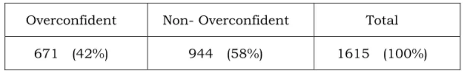
Table 2 describes the the numbers and distributions of overconfident and non-overconfident CEOs in our sample. There is only 42 percent of our sample CEOs are classified as overcon-fident. This is much smaller than the average percentage for the period 1993-2003 (61.08% accroding to Hirsh...,et al, 2012). Next, Table 3 presents the descriptive statistics of the vari-ables used in this study.

Table 2 Numbers and Distributions of Overconfident and Non-Overconfident CEOs For Good and Bad news

The table describes the numbers and distributions of overconfident CEOs in our sample. We use the options-based overconfidence measure. We calculate an average moneyness of the manager`s option portfolio for each year. Overconfident CEO takes a value 1 if a CEO postpones the exercise of vested options that are at least 67% in the money, and 0 otherwise. If a CEO is identified as overconfident by this measure, she remains so for the rest of the sample period. This treatment is consistent with the notion that overconfidence is a persistent trait. Numbers in parentheses indicate the distributions of overconfident and non-overconfident CEOs in our sample.

Overconfident Non- Overconfident Total 671 (42%) 944 (58%) 1615 (100%)

(30)

Table 3. Descriptive Statistics

The table gives the means and standard deviations of the variables used in this study. The sample consists of company issued guidance data for all nonfinancial and nonutility firms from Thomson Reuters' First Call Historical Database (FCHD) for the period 2008-2011, as during the period of global recession the revealed information is supposed to be valued most carefully. To be included in the sample, firms are required to have executive compensation details from Execucomp, accounting data from Compustat and stock returns data from CRSP. Preignition (good) and Preignition

(bad) refers to stock price trends for good and bad news, respectively. We adopt the

options-based measure of CEO overconfidence, which defines a CEO as overconfident after he holds options that are at least 67% in the money. Variable definitions are provided in the Appendix.

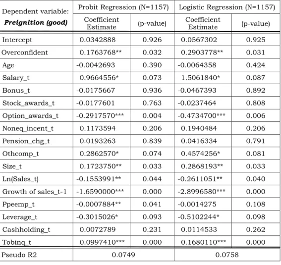
Variables Obs Mean Std. Dev. Min Max Preignition (good) 1157 0.57908 0.49392 0 1 Preignition (bad) 458 0.48908 0.50042 0 1 Overconfident 1615 0.41548 0.49295 0 1 Age 1615 56.3015 8.03532 0 84 Salary_t (%) 1615 0.21680 0.11045 0 0.61093 Bonus_t (%) 1615 0.05053 0.54978 0 20.5996 Stock_awards_t (%) 1615 0.46163 0.76259 -0.00483 11.6367 Option_awards_t (%) 1615 0.33713 0.49171 -0.09478 5.53191 Noneq_incent_t (%) 1615 0.29964 0.49257 0 5.52746 Pension_chg_t (%) 1615 0.17812 0.46120 -0.19610 6.01380 Othcomp_t (%) 1615 0.07897 0.31869 0 5.53051 Difference_t (%) 1615 0.17156 0.90985 -0.80309 14.19630 Stock Volatility_t 1615 0.44410 0.21928 0.13277 2.59440 Size_t 1615 6.78992 1.42714 2.82512 11.02950 Sales_t 1615 8345.74 25793.8 37.83800 444948 Growth of sales_t 1615 0.07389 0.16797 -0.59030 1.59712 Growth of sales_t-1 1615 0.08705 0.18634 -0.68981 1.62071 Ppeemp_t 1615 78.0401 230.748 0.72130 4079.98 Leverage_t 1615 0.31652 0.28100 0 3.10099 Cashholding_t 1615 2.35341 6.34550 0.00282 113.357 Tobinq_t 1615 4.55280 3.77025 0.25412 37.6184 3.1.3 Empirical Models Pr () = 0+ 1 + 02+ 03+  (6) where

Pr () = a dummy variable set to 1 if is equal to ; and 0 otherwise

(31)

= other compensation strucutre variables

 =firm chracterisitc variables controlling supply side, financial side, market performance.

The net benefit from increasing 4 is a sum of benefit from stock option award, implicit loss in performance bonus, and explicit cost of price manipulation. (Prediction 2) When the proportion of stock option awards increases, the net benefit of 4 inreases. Hence the probabiilty of using 4  0 will increase, and contrarily, the probabiilty of using 4  0 will decrease. Our results predict that, for good news, the probability of innoculation (in this case, 4  0) will decrease with the proportion of stock option, while for bad news, the probability of innoculation (in this case, 4  0) will increase with the proportion of stock option.

In other words, we predict that when the proportion of performance bonus increases, the probability of preignition (inoculation) will decrease (increase) for bad news.

The eﬀect of managerial overconfidence is similar to that of good news, i.e., the term Φ_1− _{will be greater than }_1− _{(Φ = 1 for non-overconfidence). Given that Φ}_1−

will be greater than expectation for good news, when we calculate the net benefit of increasing 4 the implicit loss in performance bonus will be higher with managerial overconfidence. There-fore, the net benefit of increasing 4 is lower with an overconfident manager. Ceteris paribus, the manager should decrease 4 to pull up this net benefit (by concavity). Hence, the probability of using preignition (in this case, 4  0) is higher with managerial overconfidence.

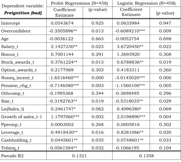
For bad news, Φ_1− _{will be greater than expectation. But managerial overconfidence will}

increase this term as Φ_1− _{is greater than }_1−_{. If the positive eﬀect from overconfidence}

dominates, then the implicit loss in performance bonus will be higher, so the net benefit of increasing 4 is less with an overconfident manager. Ceteris paribus, the manager should decrease 4 to pull up this net benefit (by concavity). Hence, the probability of using preignition (in this case, 4  0) is higher with managerial overconfidence. On the other hand, if the negative eﬀect from bad news dominates, then the implicit loss in performance bonus will be smaller, so the net benefit of increasing 4 is higher with an overconfident manager. Ceteris paribus, the manager should increase 4 to reduce this net benefit (by concavity). Hence, the probability of

(32)

using preignition (in this case, 4  0) is lower with managerial overconfidence. 2. Eﬀort and Stock Price Trend

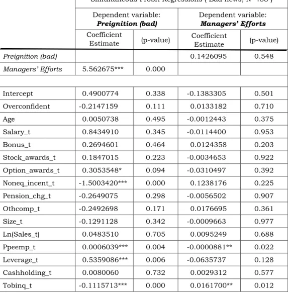
We estimate the following probability model:

 0   = 0+1 +2 ()+03+04+ (7)

where

 0_{  }

= eﬀort level, proxied by growth rate at .

  =a dummy variable set to 1 if 67% is equal to ; and 0 otherwise

 () = a dummy variable set to 1 if is equal to ; and 0 otherwise

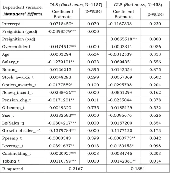
For good news (  ), since the term Φ1− will be greater than expectation, the net benefit of increasing  is higher than expectation. Ceteris paribus, the manager should increase effort to lower down this net benefit. Moreover, if preignition (in this case, 4  0) is adopted, then the net benefit of increasing 4 will increase (by the concavity of the payoff function). Altogether, the overall net benefits of increasing 4 and e will be higher than expectation. The manager needs to increase effort to lower down the overall net benefits to keep the first order condition satisfied.

On the other hand, for bad news (  ), since the term Φ_1− _{will be smaller than}

expectation, the net benefit of increasing  is lower than expectation. Ceteris paribus, the manager should decrease effort to lower down this net benefit. Moreover, if preignition (in this case, 4  0) is adopted, then the net benefit of increasing 4 will decrease (by the concavity of the payoff function). Altogether, the overall net benefits of increasing 4 and e will be lower than expectation. The manager needs to decrease effort to pull up the overall net benefits to keep the first order condition satisfied. We make the following prediction.

Prediction 6 For good news, the manager’s eﬀort level will increase with the probability of using preignition; the manager’s eﬀort level will decrease with the probability of using preignition.

(33)

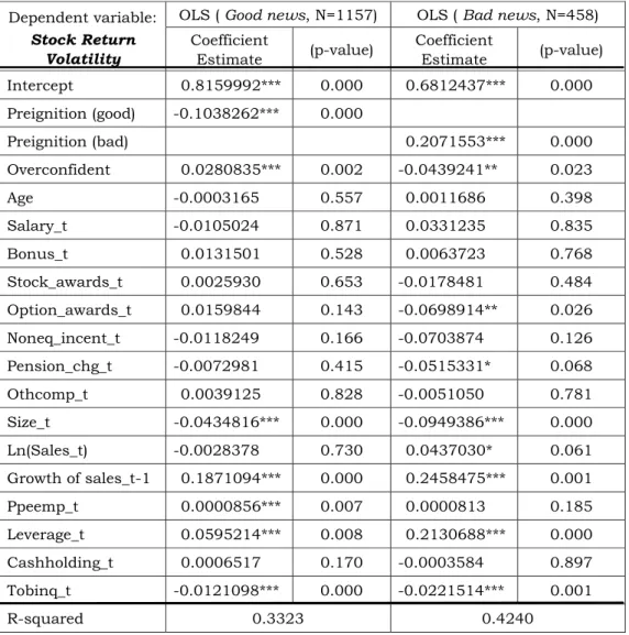
Finally, we estimate the following probability model:

  = 0+ 1 + 2 ()+ 03+ 04+  (8)

where

   =Stock return volatility

  =a dummy variable set to 1 if 67% is equal to ; and 0 otherwise

 () = a dummy variable set to 1 if is equal to ; and 0 otherwise

The final result is about stock volatility and the choice of price trend. Since the literature has documented that investors will overreact to bad news (Veronesi, 1999), we expect that the downward price trend will cause more volatility to stock return. In other words, stock volatility is negatively related to the choice of preignition for good news and positively related to the choice of preignition for bad news. Bekaert and Wu (2000) provide evidence that market-level news can create volatility feedback loops, where bad news exacerbates price responses through leverage and volatility eﬀects, while good news dampens price responses. Conrad, Cornell, and Landsman (2002) find that investors weight bad news more heavily than good news when the macro-economy is in a relatively good state. Mian and Sankaraguruswamy (2012) show that, during periods of high market sentiment, investors respond more strongly to bad vs. good news. Conversely, when market sentiment is low, investors respond more strongly to good vs. bad news.

3.2 Empirical Results

Our empirical studies test the relation between the forecast induced stock price trends, man-agement compensation structure (Prediction 2) and managerial overconfidence (Prediction 4), and how the choices of price trend and managerial overconfidence affect the manager’s effort decision (Predictions 3 and 5). Finally we test whether the choice of stock price trend will affect the companies’ stock volatility.