Call Admission and End-to-end delay Allocation for Fair Queueing Networks

全文

(1)Call Admission and End-to-end delay Allocation for Fair Queueing Networks W. C. Chiang. Y. P. Chu Department of applied math. of National Chung Hsing University. C. L. Lee. Y. H. Huang. Department of Department of Infor Department of Infor applied math. of -mation Management -mation Management National Chung of HsiuPing Institute of HsiuPing Institute Hsing University. No. 250, KuoKuang No. 250, KuoKuang No. 11, Gungye Rd., No. 11, Gungye Rd., Rd., Taichung City, Rd., Taichung City, Dali City, Taichung, Dali City, Taichung, Taiwan 412 Taiwan 412 Taiwan 401 Taiwan 401 ypchu@amath.nchu wzjiang@vghtc.gov.t cllee@mail.hit.edu.t ehhwang@mail.hit.e w w du.tw .edu.tw Abstract. traffic shaper and a fair queueing scheduler.. 1. Introduction. Many multimedia applications, including audio and video, require quality of service（ QOS）. The newly applications of high-speed. guarantees from network. A typical user is only. integrated service networks is to provide quality. concerned with the QOS requirements on end. of service guarantees, such as packet loss ratio,. -to-end basis and does not care about the local. end-to-end delay, and throughput, to follows. switching node QOS. In this paper, we propose. requiring different classes of services. Hence,. a general framework to map the end-to-end. the network needs to reserve resources, for. QOS requirement into the local switching node. example, buffer and bandwidth, to promise the. QOS requirements. Most of recent research. performance requirements for each application.. efforts only focus on worst-case end-to-end. There are two categories of guaranteed-service. delay bound but pay no attention to the problem. models in order to support guaranteed-service. of distributing the end-to-end delay bound to. applications [4,5]. One is the deterministic. local switch node. Therefore, we focus on the. guaranteed service. This model can promise the. local switching node QOS requirement and. worst-case performance bound for all packets in. design a novel QOS requirement allocation. the same connection and get better quality of. scheme to get better performance. Using the. service. The other is the statistical guaranteed. number of maximum supportable connections as. service. This model only promises probabilistic. the performance index, we derive an optimal. performance. delay allocation（ OPT） policy. In addition, we. but. gets. the. higher. utilization from network. No matter what the. also design an analysis model to evaluate the. service is deterministic or statistical, the. proposed allocation scheme and equal allocation. improvement of network utilization is an. （ EQ） scheme, which apply to the switching. important consideration.. nodes along the flow’ s path with the Rate -controlled scheduling architecture, including a. Recent research efforts only focus on 1. PDF 檔案以 "PDF 製作工廠 " 試用版建立. bound. http://www.fineprint.com.

(2) worst-case delay bound but pay no attention to. Rated-controlled service architecture consists of. the problem of distributing the end-to-end delay. a traffic shaper and a scheduler. The traffic. bound. node. shaper can shape the incoming traffic at each. the. switching node as they enter the network by. end-to-end QOS requirements into the local. controlling the output time of packets in a traffic. switching node QOS requirements is the one of. shaper. Here, we use fair queueing as the. the. for. scheduler because the fair queueing is easy to. maximizing network utilization. In order to. implement and offers a diverse set of delay. improve the network utilization, when the new. bounds to connections. In addition, routing of. connections is admitted and enter to the network. connections is not addressed. We assume that. after admission control, they equally allocate the. the routing decision has already been made. This. excess delay and reserve the same bandwidth at. allows us to focus on the problem of resource. each switch along the flow’s path. In [5], the. allocation without having to address the. author has proposed a scheme that first. combined problem of route selection and. computes the aggregated local worst-case delay. resource allocation. In section 2, we define our. bound, and calculates the difference between the. system architecture and show how to compute. aggregated value and the application-required. the. delay. Then, the excess value is equally assigned. architecture.. to the local switching node along the flow’s path.. admission control procedure and analyze the. However, it cannot improve the network. allocation policy. Section 4 will give some. utilization efficiently. Our approach is based on. important numerical results. Section 5 is our. the mapping of QOS requirement into local. conclusion and future direction.. to. the. local. [2,3,7-9,13,14,16-18].. most. switching. How. important. to. map. considerations. end-to-end. resources to be reserved at each scheduler. In. How to allocate the end-to-end. S. delay to the local delay? l. Section. 3. bound. under. this. will. propose. the. 2. System Architecture. this paper, we addressed the following issues: l. delay. A1. In. 1. A2. Dn(In||A1) Dn(A1,A2). How many connections for this type. 2. AK. K. D. Dn(AK-1,AK) DnK. Fig. 1 The end-to-end delay computation model. of application can be allowed into the network under the different. Traffic Shaper 1. allocation policies? l. Input traffic. Traffic Shaper 2. .... Which. factor. will. affect. the. Scheduler Traffic Shaper N. allocation policy? Rate Controller. We. consider. scheduling. the. policy. Fair. queueing. [3-5,12].. We. packet use. Fig. 2 The architecture of the switching node. the. Rated-controlled service architecture to prevent the. traffic. distortion. [11,15,19,20].. In this section, we described our system. The. architecture 2. PDF 檔案以 "PDF 製作工廠 " 試用版建立. http://www.fineprint.com. and. the. computation. of. the.

(3) end-to-end delay bound. We first add a policing. the output of the shaper Anm . From the fig. 1,. function for every connection at the entrance of. we find that the end-to-end delay Dn of the. the network to shape the incoming traffic. We. connection n with the input traffic envelope. define I n ( s, s + t ) be the number of bits that. I n (t ) is. arrive in the interval [ s, s + t ) for connection n. Let. I n ( s, s + t ) = 0. t≤0 ,. for. otherwise. K −1. Dn = Dn ( I n || An1 ) + ∑ Dn ( Anm , Anm +1 ) + DnK .. I n ( s, s + t ) > 0 for t > 0 , and σ n , ρ n , l ≥ 0 ,. m =1. such that From equation (1), we have. I n ( s, s + t ) ≤ σ n + l + ρ n t = I n ( t ) K −1. K −1. m =1. m =1. Dn ≤ Dn ( I n || An1 ) + ∑ Dnm + ∑ Dn ( Anm || Anm +1 ) + DnK .. We call I n (t ) the input traffic envelope. Where. σ n is the bucket size and ρ n is the average arrive rate [11,15]. We assume all packets have. We will compute the end-to-end delay Dn .. the same length and equal to l . Therefore, we. First, we consider Dn ( Anm || Anm +1 ) . Note that if. use the leaky bucket model to characterize the. traffic. input traffic. Suppose one application wants to. D( A || B ) = 0 . Therefore, we use the same. enter the network , and this application has the. parameter for all traffic shaper at each switching. I n (t ) . Consider the. node, that is, Anm (t ) = Anm +1 (t ) = An (t ) , for each. input traffic envelope. end-to-end delay as the application’s QOS. A (t ) ≤ B ( t ). envelope. ,. then. m=1,2,… , K-1, then. requirement. For a single connection n that K −1. passes through K switching nodes as in Fig. 1,. ∑D (A n. we assume that before the packets enter the. m n. || Anm +1 ) = 0. m =1. scheduler of node m, they pass through the traffic shaper Anm as the fig.2 shown. Moreover,. Reference [17] has shown that use the identical. we assume the propagation delay for each. traffic shaper An to replace the various traffic. m n. m +1 n. output link is zero. Let Dn ( A , A. ) denote. shapers for each switching node will have the. the delay that a packet from connection n. same worst-case end-to-end delay bound. Hence,. experiences between the time it exits shaper. the worst case end-to-end delay bound Dn is. m n. A. m +1 n. and A. , for the fig. 1 described. Ref. [10]. given by. has shown that K. D n ≤ D n ( I n || An1 ) + ∑ Dnm. Dn ( Anm , Anm =1 ) ≤ Dnm + Dn ( Anm || Anm +1 ), ········(1) Dnm. m =1. is the upper bound of the. Secondly, we consider Dn ( I n || An1 ) . We. scheduling delay at node m, and Dn ( Anm || Anm +1 ). assume I n (t ) = σ n + l + ρ n t . However, how to. denote the upper bound of the delay in the. assign the parameter of traffic shaper An ? The. Where. m +1 n. shaper A. m +1 n. where the input of shaper A. is. choice of this parameter will affect the 3. PDF 檔案以 "PDF 製作工廠 " 試用版建立. http://www.fineprint.com.

(4) end-to-end delay bound. In the following, we. K. Thirdly, we consider. will discuss this problem. We first let. ∑D. m n. . It is the. m =1. scheduling delay bound at each switching node.. An (t ) = σ n + hn t . For the. Since the input of the scheduler is the output of. traffic of the sources entering the first shaper, it. the traffic shaper An . If we let the service rate. must satisfy that the average output rate is great or equal to average input rate,. of switching node m for the connection n is g nm. hn ≥ ρ n .. and the scheduling algorithm at each switching. Otherwise, it will result in an infinite delay at. node is fair queueing, then the worst scheduling. the first shaper. For the stability condition, we. delay bound for connection n at the switching. have hn ≤ r m , at each switching node m, where. node m is [2,9,13,19]. r m is the available output capacity at switching node m. Therefore, for the envelope of the. Dnm =. traffic shaper, we have the following inequality. ρ n ≤ hn ≤ r m. σn l + m .········································(3) m gn C. Where C m is the capacity of the output link for switching node m, and l is the packet length.. Note that the service rate g nm for the connection. Finally we can get the end-to-end delay bound. n at switching node m must satisfy following. Dn for connection n is. equation.. Dn =. hn ≤ g nm ≤ r m Hence, we can define hn = ρ n , and the above. l + ρn. K. σn. ∑( g m =1. m n. +. l ) ·························(4) Cm. In next section, we propose an admission control. equation will become. procedure that we used by this result and analyze. ρ n ≤ g nm ≤ r m . ··········································(2). two. allocation. policies. for. the. end-to-end delay requirement.. 3. The analysis model. Since this assignment can have the maximum flexibility for the allocation of the service rate. Take the service rate constraint in eq. (2). g nm at each local switching node, even it may. into eq. (3), we define. not have the optimal (minimum) end-to-end delay bound. Because the evaluation for the max d nm =. different delay allocation policies is the purpose. σn l + , ··································(5) ρn C m. of this paper, we believe this restriction will not affect our results of evaluation. Now we define. and. An (t ) = σ n + ρ n t . And then. Dn ( I n || An1 ) =. min d nm =. I n (t ) − An1 (t ) l = , ρn ρn 4. PDF 檔案以 "PDF 製作工廠 " 試用版建立. http://www.fineprint.com. σn l + , ·································(6) rm C m.

(5) Where max d nm is the maximum value of delay. were many admission control methods proposed. bound from connection n at node m, and. [1,6,12], we adopt our admission control. min d. m n. is the minimum value of delay bound. procedure as follows:. from connection n at node m.. (1) If. Consider a single source-destination route,. rejected,. where there are K nodes. If a connection n wants. (2) If d > Dmax , then the connection can be. to enter the network with the traffic envelope being. I n (t ) = σ n + l + ρ n t ,. t≥0. d < Dmin , then the connection is. accepted and we allocate the local delay. and the. with the value of. end-to-end delay requirement is D. We compute the maximum value and minimum value of. σn l + ρn C m. for each. switching node m.. end-to-end delay Dnmax and Dnmin based on eqs.. (3) If Dmin ≤ d ≤ Dmax , then the connection can. (4), (5), and (6) with. also be accepted and we can make the Dnmax =. l + ρn. proper allocation policy for the end-to-end. K. ∑ max d. m n. delay requirement.. m =1. In our analysis model, we used the fair and. queueing scheduler as our scheduling algorithm, unlike FCFS scheduler, it service packets with D. min n. l = + ρn. K. ∑ min d. m n. separate queues for different connections even. m =1. in cross traffic model. That is, cross traffic model is only a combination of several tandem That is, under the condition of the input traffic. models. Therefore, it is enough to show the. envelope being I n (t ) = σ n + l + ρ n t , t ≥ 0 , if. differences for different allocation policies. the end-to-end delay requirement of the new connection. [D. min n. n. is. belong. to. the. under tandem model. In the following, we. interval. , Dnmax ] , it implies the network can support. analyze two different allocation policies: equal allocation (EQ) and optimal allocation (OPT). the need for this connection. The connection. policy under a tandem network model.. will be accepted and the excess delay should be allocated properly for network utilization. If the. 3.1 EQ policy. end-to-end delay requirement D is larger than. Assume that the maximum value of. the maximum value of end-to-end delay Dmax ,. end-to-end delay upper bound from node 1 to. that means the delay requirement of the new. node K is. connection is low, the network also can accept. Dmax , the minimum value of. end-to-end delay lower bound is Dmin . The. the connection and must allocate the local delay. end-to-end delay requirement for the new class. σn l + with the value for each switching ρn C m. application is D, Dmin ≤ D ≤ Dmax . First, we consider an EQ policy that assigns an equal. node m to ensure the schedulable region under. amount. fair queueing scheduler. However, even there 5. PDF 檔案以 "PDF 製作工廠 " 試用版建立. http://www.fineprint.com. of. the. extra. end-to-end. delay.

(6) requirement for a connection to each switching. Where N s is the maximum number of new. node. In the following we will calculate the. connection under stability condition. And then,. number of allowable connections, N EQ , for this new class under the EQ policy. With this value,. Cm −. we can evaluate the allocation policy and derive. Ns <. the delay allocated to node m. Let ∆d m be the. n −1. ∑ρ i =1. ρn. i. ,. amount of the extra delay at node m, then. ∆d m =.  m n −1   C − ρi  i =1 Ns =   .···································(9) ρ   n  . ∑. d − Dmin , K. Since the amount of the extra delay is allocated to each switching node equally. ∆d m = ∆d , for m = 1,2 ,K , K . Let N m. Combine eqs (8), (9) , then we have. be the number of. N EQ = min{N f , N s }. ·································(10). supportable connections for node m, and. min d nm be the minimum value of delay bound for connection n at node m. Consider the worst. Finally, Replacing N m of eq.(7) with N EQ , we. case, then. can derive the delay that is allocated to node m. 3.2 OPT policy. l  σ min d + ∆d = N  mn + m  , ·················(7) C  r m n. m. Next, we consider the optimal allocation policy. We want to determine the value of the. We have. allocated delay that maximize the number of connections. Let N be the maximal number of connections for the new class. And let ∆d m be. min d nm + ∆d N = , ∀m = 1,2 ,K , K , σn l + rm C m m. the amount of extra delay at node m in OPT policy, then. Let. K. ∑ ∆d. m. = D − Dmin ,. m =1. N f = min{N 1 , N 2 ,K , N K } .·························(8) Where D is the end-to-end delay requirement of For the stability condition, the sum of all. new application, and Dmin is the minimum. arriving rate must be no more than the capacity. value of end-to-end delay.. of all the links. Therefore, For each switching node m considering the worst case,. n −1. ∑ρ. + N s ρ n < C , ∀m = 1,2, K, K , m. i. i =1. 6. PDF 檔案以 "PDF 製作工廠 " 試用版建立. http://www.fineprint.com.

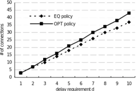
(7) l  σ min d nm + ∆d m = N  mn + m  , ···············(11) r C  . Finally, Replacing N of eq.(10) with N OPT , we can derive the delay that is allocated to node m.. Then,. 4 Numerical results N=. In this section, we present some numerical. min d nm + ∆d m , σn l + rm C m. examples to compare the performance of the EQ and. OPT. delay. allocation. polices.. Two. performance measure indexes are adopted to decide the efficiency and optimality of the. We let. allocation utilization,.    min d nm + ∆d m  Nf =   .····························(12)  σn + l   r m C m . policies. in. One. terms. is. of. the. the. network. number. of. supportable connections. Moreover, another index is the relative gain (RG) to evaluate the optimality of the allocation policy.. N. For the stability condition, the sum of all. 1. C1. 2. C2. 3. C3. D. arriving rate must be no more than the capacity Fig.3 Tandem model. of all the links. Therefore,. Fig. 3 shows this model consisting of a n −1. ∑ρ. i. single source-destination pair of nodes in an. + N s ρ n < C m , ∀m = 1,2 ,K , K ,. ATM network. Each packet be assigned to the. i =1. same size l = 53 bytes. Suppose the network has Where N s is the maximum number of new. three nodes and only a single route. The capacity. connection under stability condition. And then,. for the links of all nodes is 300 packets per second, and the remained capacity for the link of. Cm − Ns <. node 1 and node 3 are 150 packets per second.. n −1. ∑ρ i =1. ρn. i. The input traffic follows the leaky-bucket. ,. constrained with burst size σ = 10 packets and average rate ρ = 5 packets per second. The value of σ must be great than l to ensure that.  m n −1   C − ρi  i =1 Ns =   . ·································(13) ρn    . ∑. at least one packet can be filtered by the traffic shaper. With the remained capacity for the link of node 2 being 120 packets per second, we. Combine eqs (12), (13), then we have. calculate the number of supportable connections. N OPT = min{N f , N s }. ································(14). for EQ and OPT delay QOS allocation policies by eq. (10) and (14) respectively. 7. PDF 檔案以 "PDF 製作工廠 " 試用版建立. http://www.fineprint.com. Fig. 4 shows.

(8) the variation in the network utilization over. connections over the end-to-end delay require. end-to-end delay requirement.. -ment in the network model with the remained. The end-to-end. delay requirement D for new connections is. capacity of node 2 varied.. By the way, we can. ranged from 1 to 6.6.. From the results we find. observe the variation of the network utilization. that the OPT allocation policy performs better. over the end-to-end delay requirement when the. than the EQ policy because the number of. bottleneck link capacity changed.. connections admitted by the former is far more. the OPT policy performs better than the EQ. than the later in each delay bound in the. policy under any network conditions.. We find that,. end-to-end delay requirement. It implies that the OPT policy has higher network utilization than EQ policy. This is because that OPT policy is. EQ C2 = 120. OPT C2 = 120. EQ C2 = 60. OPT C2 = 60. 50 # of connections. based on each node’s situation to allocation local delay, so it can prompt more network performance than EQ policy which allocate local delay equally.. 40 30 20 10 0 1. 2. 3. 50. 4 5 6 7 8 delay requiremwnt d. 9. 10. # of connections. 45 40. EQ policy. 35. OPT policy. Fig. 6 RG vs. bottleneck ratio. 30 25. We compute the relative gain (RG) for OPT. 20 15. policy relative to EQ policy with different. 10 5. bottleneck ratio.. 0 1. 2. 3. 4 5 6 7 delay requirement d. 8. 9. The RG is defined as follow:. 10. RG =. Fig. 4 Delay requirement vs. no. of connection. N OPT − N EQ N EQ. .. 0.9. The bottleneck ratio of bottleneck link. 0.8 0.7. capacity with the other link capacity, and is. Relative Gain. 0.6. ranged from 0.13 to 1.. 0.5. d is fixed at three.. 0.4 0.3. The delay requirement. From fig. 6 we find that, the. smaller the bottleneck ratio the larger the gain,. 0.2. i.e., the OPT policy is far better than the EQ. 0.1. policy,. 0 0.13 0.20 0.27 0.33 0.40 0.47 0.53 0.60 0.67 0.73 0.80 0.87 0.93 1.00 Bottleneck ratio. especially. when. the. bottleneck. bandwidth is smaller than the other link. Fig. 5 No. of admitted connections vs. the. bandwidth. That is because we need to allocate. end-to-end delay requirement with the different. resources carefully when the network resources. remained capacity of node 2. are restricted. According to the results, OPT policy can support more connections and utilize. Fig. 5 shows the number of admitted 8. PDF 檔案以 "PDF 製作工廠 " 試用版建立. http://www.fineprint.com.

(9) Packet Scheduling Algorithm: Minimum. network resources efficiently.. Starting-Tag. 5. Conclusion. Fair. Transaction. on. Queueing”,. IEICE. Communications,. vol.. E80-B, no.10 October 1997.. In this paper, we applied the rate-controlled [3]. service architecture with the fair queueing. A. Demers, S. Keshav, and S. Shenker,. packet-scheduling algorithm to evaluate the. "Analysis and simulation of fair queueing. effects of the allocation policies. With the. algorithm”, Journal of Internetworking. number of maximum allowable connections as. Research. the performance index, a solution for an optimal. October 1990. [4]. delay allocation was derived. The results of this. and. Experience,. pp.. 3-26,. D. Ferrari and D. Verma, "A Scheme for. analysis have shown the relationship of the. Real-time. delay to the number of maximum allowable. Wide-Area. connections. In addition, from the numerical. Selected Areas of Communications, 8(4),. results, we have found that the bottleneck ratio. pp.368-379, April 1990. [5]. will influence the performance of the allocation. Channel. Establishment. Network”,. IEEE. in. Journal. D. Ferrari, "Real-time communication in an Internetwork”, Journal of High Speed. policy.. Network, vol. 1, no. 1, pp. 79-103, 1992. Of. course,. the. local. allocation. of. [6]. end-to-end QOS requirement must be combined. V. Firoiu, J. Kurose, D. Towsley, "Efficient admission control for EDF schedulers",. with an admission control algorithm. When the. Proceedings of IFCOM'97, Apr. 1997.. traffic model parameters, link bandwidth in each. [7]. node along the path connection pass through,. S. Golestani, "A self-clocked fair queueing scheme. and propagation delay are known, the network. for. broadband. applications”,. Proceedings of IEEE INFOCOM '94,. can compute the local QOS requirement in each. Toronto, pp. 636-646, June 1994.. node according to the analysis results in this. [8]. paper.. S. Golestani, "Network delay analysis of a class of fair queueing algorithms”, IEEE Journal Selected Areas of Com., vol. 13,. The performance index may be changed. pp. 1057-1070, August 1995.. depending on the various requirements of the [9]. network and end-users. In the future, we will. P.. Goyal,. H.. Vin,. and. H.. Cheng,. determine the diverse performance index to. "Start-time Fair Queueing: a scheduling. design and evaluate a method for local QOS. algorithm for integrated services packet. allocation.. switching. [2]. IEEE/ACM. Transaction on Networking, vol. 5, no. 5,. References [1]. networks”,. pp. 137-150, October 1997.. The ATM Forum, "Traffic management. [10] L. Georgiadis, R. Guerin, and V. Peris, and. specification version 4.1", AF-TM- 0121.. K. N. Sivarajan, "Efficient network QOS. 000, Mar. 1999.. provisioning based on per node traffic. Y. P. Chu and E. H. Hwang, "A New. shaping", 9. PDF 檔案以 "PDF 製作工廠 " 試用版建立. http://www.fineprint.com. IEEE/ACM. Trans.. on.

(10) pp.227-236 1993. Networking, Vol.4, No.4, pp.482-501, Aug.. [19] H.. 1996.. Zhang,. guaranteed. [11] E. Kinghtly and H. Zhang, "traffic. "Service. disciplines. performance. service. for in. characterization and switch utilization. packet-switching networks.", Proceedings. using. of IEEE, Vol.83, No.10, pp.1374-1399,. deterministic. bounding. interval. Oct., 1995.. dependent traffic models”, Proceedings of. [20] H. Zhang and D. Ferrari, "Rate-controlled. IEEE INFOCOM'95, April 1995. [12] J. Liebeherr, D. E. Wrege, and D. Ferrari,. service disciplines.", Journal of High. "Exact admission control for networks. Speed Networks, Vol.3, No.4, pp.389-412,. with bounded delay services", IEEE/ACM. 1994.. Trans. on Networking, Dec. 1996. [13] A. Parekh and R. G. Gallager, "A generalized processor sharing approach to flow. control. networks:. in. The. integrated. services. single-node. case”,. IEEE/ACM Transaction on Networking, vol.2, no.2, pp.344-357, June 1993. [14] A. Parekh and R. G. Gallager, "A generalized processor sharing approach to flow. control. networks:. The. in. integrated. services. multiple-node. case”,. IEEE/ACM Transaction on Networking, vol.2, no.2, pp.137-150, April 1994. [15] J. Turner, "New directions in communica -tions (or which way to the information age?)”, IEEE Communication Magazine, vol. 24, pp. 8-15, October 1986. [16] G. G. Xie and S. S. Lam, " Delay guarantee. of. VirtualClock. server”,. IEEE/ACM Transaction on Networking, vol.3, no.6, pp.683-689, December 1995. [17] L. Zhang, "VirtualClock: a new traffic control algorithm for packet switching networks”, ACM Transaction on Computer Systems, vol. 9, no. 1, pp 3-26, 1990. [18] H. Zhang and D. Ferrari, "Rate-controlled static priority queueing”, Proceedings of the IEEE INFOCOM '93, San Francisco, 10. PDF 檔案以 "PDF 製作工廠 " 試用版建立. http://www.fineprint.com.

(11)