A DATA mining Procedure Using Neural Network- Self Organization Map and Rough Set to Discover Association Rules

全文

(1)A DATA mining Procedure Using Neural Network- Self Organization Map and Rough Set to Discover Association Rules S. Wesley Changchien and Tzu-Chuen Lu Department of Information Management Chaoyang University of Technology, Taichung, Taiwan, R.O.C E-mail: {swc, s8814602}@cyut.edu.tw Abstract Modern enterprises are usually equipped with database and data warehouse for data storage and analysis, but they are of less use without insight and intellectual analysis. Data mining techniques are popular and often used to find knowledge from enterprise data store and thus support to make better decisions. Data mining by automatic or semiautomatic exploration and analysis on large amount of data item set in a database can discover significant patterns and rules underlying the database. However, for large non-homogeneous data item set, direct extraction of rules with traditional data mining techniques may be useless or meaningless. The purpose of the paper is to propose a data mining procedure for database with large amount of transaction records. The data mining procedure consists of two methods. One is a neural network, Self-Organization Map (SOM), which performs an affinity grouping tasks on large amount of database records. The other is rough set theory, which extracts association rules for each homogeneous cluster of data records. An implemented system was applied to a sample from purchase records of a database for illustration. Keywords: Data mining, neural network, SOM, Rough set, association rules 1.. Introduction. In today’s competitive business marketing, there is a number of reasons of utilizing data mining tools: ever-increasing amount of data, business reengineering and organizational decentralization, faster product cycles and globalization and enterprise topologies, etc. [7]. Enterprise managers usually use data mining tools to improve their services and make better decisions. Which customer is loyal? What Products are usually purchased together? What is the next product or service this customer will acquire? These questions interest managers very much. In general, OLTP (On-Line Transaction Process) and OLAP (On-line Analytical Processing) are often used to answer these questions. These tools although provide ways of analyzing data following the. rules defined by users, but do not creatively derive empirical rules and conclude themselves. Therefore it is of little use for managers without intelligence. Intelligence allows us to devise rules, creating new ideas, and make predictions for the enterprise [4,7,8]. Data mining techniques can perform automatic or semiautomatic exploration and analysis of large quantity of data in order to discover meaningful patterns or rules. Data mining takes two forms: verification-driven data mining, which is a top-down approach that attempts to substantiate or disprove preconceived ideas, and discovery-driven data mining, which extracts information automatically from data [8,16]. Both data mining forms are to achieve some of the data mining tasks including finding association rules, clustering, classification and estimation, etc. [1,2,3,5,6,14,19,21,22]. When the managers try to understand more about their customers, their intuition is to separate the customers into smaller groups, each of which can be explained more specifically. In marketing terms, subdividing the population according to variables already known to be good discriminators is called “Clustering” [8]. There are numerous of clustering algorithms, one of which is Self-Organizing Map (SOM), a neural network that can recognize unknown patterns in the data [11,16]. When training data sets are fed into the network, SOM will compute and come up with a winner node. The network will adjust winner node and neighborhood weights accordingly. Training continues until it converges. Then SOM will then be capable of determining which cluster the new input belongs to. Clustering techniques can separate data items into clusters of items, other methods then can be applied to figure out the underlying features for each cluster in terms of association rules. Knowledge is usually represented in the form of rules – rules deducting the degree of association between two variables, rules mapping data into predefined classes, rules identifying a finite set of categories or clusters to describe the data, etc. Mining association rules has attracted a significant amount of researchers [9,12,13,17,18,20]. Finding patterns in a database is the fundamental operation behind most of the common data mining tasks, including mining of association rules and sequential patterns. Rough set theory is used for approximation of a concept.

(2) that uses lower and upper sets of the concepts. When we inspect the data mining queries with respect to the rough set theory, dependency analysis and classification of data items are well investigated. The associations between values of an attribute can easily be solved by the rough set theory [10,15]. Pawlak proposed rough set theory in 1982. This theory is an extension of set theory for the study of intelligent systems with incomplete information [16]. Let U be a finite, nonempty set called the universe, and let I be an equivalence relation on U, called an indiscernibility relation. I(x) is an equivalence class of the relation I containing element x. The indiscernibility relation is meant to capture the consequence of inablility to discern in view of the available information. There are two basic operations on sets in the rough set theory, the I-lower and the I-upper approximations, defined respectively as follows:. 2.1 Step 1-Selection and Sampling. I* ( X ) = {x ∈ U : I ( x) ⊆ X }. (1). 2.1.2 Selecting dimensions. I * ( X ) = {x ∈ U : I ( x) ∩ U ≠ φ }. (2). Usually in order to define a set we use a confidence function. The confidence function is defined as follows: CF ( x ) =. Num ( X ∩ I ( x )) where CF ( x) ∈ [0,1] , (3) Num ( I ( x )). Where Num( X ∩ I ( x)) is the number of objects that occur simultaneously in X and I(x), and Num ( I ( x )) is the number of objects in I(x). Confidence function can be used to redefine equations (1) and (2) as follows: (4) I ( X ) = {x ∈ U : CF ( x) = 1} *. I * ( X ) = {x ∈ U : CF ( x) > 0}. 2.1.1 Creating fact table There are a lot of tables in enterprise’s database. The fact tables that interest the managers are created according to the mining purpose. For example, there may be vendor, product, sale, and customer tables in a database (Figure 2). User then selects dimensions from the fact table next.. When managers want to analyze their company’s general association rules, they can choose dimensions from the fact table. Our implemented system will analyze a certain dimension and find out the relationships among the attributes. For example, a manager can select sale table to find what relationships the attributes have in between. 2.1.3 Selecting dimension attributes Sale table has multiple attributes. But not all of those attributes fit into the analysis and attributes are of different levels of importance to the manager. Therefore our implemented system allows user to choose some of the attributes and set different weights to selected attributes.. (5). The value of the confidence function denotes the degrees of how the element x belongs to the set X in view of the indiscernibility relation I. The purpose of this paper is to discover association rules from a database with large number of data records. Before discovering association rules we first preprocess our database records into clusters. This paper proposes a procedure by applying a neural network SOM first for clustering, and then using rough set theory to discover association rules. 2.. Database consists of current detail data, history data, summarized data and metadata, etc. Step 1 selects target tables, dimensions, attributes, and records for data mining. Step 1 consists of four activities: creating fact table, selecting cause and result dimensions, selecting dimension attributes, and filtering data.. Proposed Data Mining Procedure. Data mining is an interactive and iterative process involving numerous steps. Fayyad [4] outlines a practical view of data mining process. Figure 1 outlines the data mining steps. Following the data mining steps, we propose a procedure of data mining for large amount of data set as follows.. 2.1.4 Filtering data In order to get the right data, user can retrieve data with constraints such as the range of an attribute. This step also involves in removal of noises or handling of missing data fields. User can also take random sample or select part of records from database for analysis. For example, if a manager selects sale dimension then he can select dimension attributes including customer number, product number, kind of product, department, price, quality, etc. According to the corresponding attribute importance levels, we set their weights. Below we suppose that a manager selects DEPT and AMT two attributes (Table 1), where att j indicates attribute j, j ∈ [1, m] , and wegt j indicates weight j, j ∈ [1, m] , where m is the total number of attributes selected..

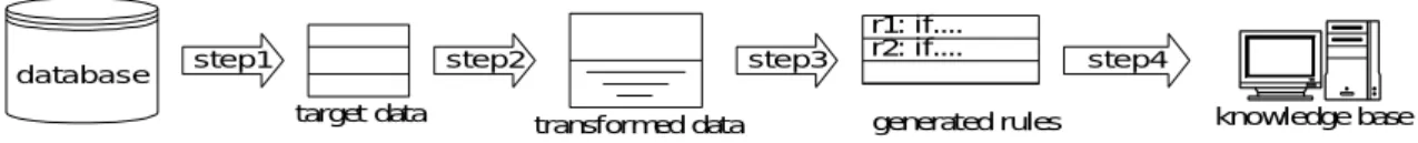
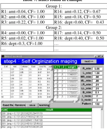
(3) step1. database. step2 target data. step3 transformed data. r1: if.... r2: if.... generated rules. step4 knowledge base. Figure 1. Data mining steps Table 1. An example of selected attributes and weights. Attribute. AMT( att1 ). DEPT( att 2 ). Weight. 0.4 ( wegt1 ). 0.6 ( wegt2 ). VENDOR CID char(10) CNAME char(50) OWNER char(12) CADDR varchar CTEL char(10) CDISCOUNT decimal CTAX decimal. PRODUCT PID LGNO MGNO BARCODE SPECIFICATION UNIT PRICE COMPANY. SALE SID char(10) SDATE date SPID char(10) SQTY integer SDICOUNT decimal SPERSON char(10). If the attribute is non-numerical then user can design data transformation scale. For instance, attribute DEPT in Table 1 is not numerical. We thus need to transform it into normalized numerical response value. When all attributes have the same measurement and ranges, we then can proceed to the next data mining process. 2.3 Step 3 Data Mining Using SOM and Rough Set. FACT_TABLE CUSTOMER char PRODUCT char COMPANY char SALE char char(13) char(5) char(5) char(13) varchar char(5) decimal char(10). Theory CUSTOMER ID char(10) NAME char(12) BIRTHDAY date PID char(10) INTERESTING char(25) ADDR varchar DISCOUNT decimal(2). Figure 2. Fact table for a sales MIS. Before proceeding data mining on data set we should normalize and scale data if it is necessary. Because this paper uses neural network for data mining preprocessing, we transfer data into values between 0 and 1. Here two different formulas can be used to transfer data. (1) Numerical If the attribute is numerical then use the following equation (valuejk − min(att j )) (max(att j ) − min(att j )). * wegt j ,. In this paper, we focus on clustering and association rule generation in data mining tasks. We use a neural network SOM for clustering. After the data are analyzed and clustered by SOM, rough set theory is used to discover association rules. 2.3.1 SOM. 2.2 Step 2-Transformation and Normalization. response _ valuejk =. (2) Non-numerical. (6). where th response _ value jk is the normalized value for the j. attribute of record k, k ∈ [1, p ] , th min(att j ) is the minimum value of the j attribute, th max( att j ) is the maximum value of the j attribute, and th val (att jk ) is the original value of the j attribute of record. k. Since the attribute type of AMT in Table 1 is numerical, we can use equation (6) above for normalization.. Kohonen proposed SOM in 1980. It is an unsupervised two-layer network that can recognize a topological map from a random starting point. By SOM we can cluster enterprise’s customers, products, suppliers, etc. According to different clusters’ characteristics, different marketing strategies may be adopted by making use of the corresponding discovered association rules. In SOM network, input nodes and output nodes are fully connected with each other. Each input node contributes to each output node with a weight. Figures 3 and 4 are the network structure and flow chart for SOM training procedure, respectively. In our developed system user can assign different numbers of output nodes (cluster number), learning rate, radius rate and converge error rate, etc. Users could also be compliant with default assignment of cluster number. In the simple example in Table 1, SOM has two input nodes: DEPT and AMT. Output nodes are set to be nine clusters. SOM network first determines the winning node using the same procedure as the competitive layer. Then the weight vectors for all neurons within a certain neighborhood of the winning neuron are updated. After the SOM network converges, we use those weights to split the data set in dimension table. According to the weights, data items can be assigned to their corresponding clusters..

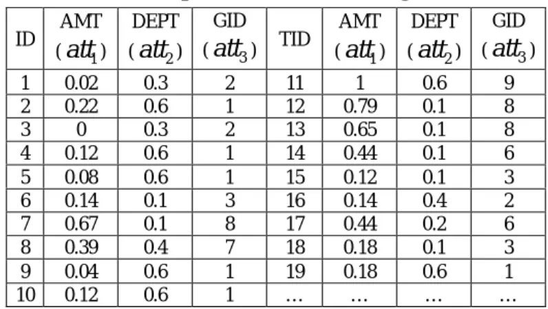
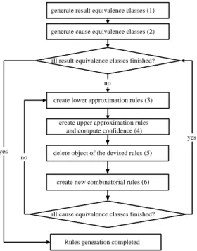
(4) Table 2. Sample records and clustering results AMT. Figure 3. The neural network of SOM setup network. randomly assign weights. set the coordinate values of output nodes. GID. AMT. DEPT. GID. ( att3 ). TID. ( att1 ). ( att 2 ). ( att3 ). 2 1 2 1 1 3 8 7 1 1. 11 12 13 14 15 16 17 18 19 …. 1 0.79 0.65 0.44 0.12 0.14 0.44 0.18 0.18 …. 0.6 0.1 0.1 0.1 0.1 0.4 0.2 0.1 0.6 …. 9 8 8 6 3 2 6 3 1 …. DEPT. ID. ( att1 ). ( att 2 ). 1 2 3 4 5 6 7 8 9 10. 0.02 0.22 0 0.12 0.08 0.14 0.67 0.39 0.04 0.12. 0.3 0.6 0.3 0.6 0.6 0.1 0.1 0.4 0.6 0.6. rules. For example, GID = 1 ⇒ X 1 = {Obj. input a set of attributes. no. cimpute the winning node. update weights and radius Process. converged ?. update learning rate and radius rate yes. end. Figure 4. Flow chart for SOM training procedure 2.3.2 Rough set Table 2 presents the records sampled from our purchase database. The attributes of the records were normalized and clustered, where GID is the cluster number and TID is the transaction identification number. Figure 5 shows the flow chart of implementing rough set. The steps are described as follows. (1) Generate result equivalence classes Let X i denote the result equivalence class as a set of objects for cluster i. Table 3 lists some of the results equivalence classes. (2) Generate cause equivalence classes. (4). , Obj. (5). , Obj. (9). , Obj. (10 ). , Obj. (19 ). A23 * = {Obj } ⇒ “Insert this into the lower rule table: IF amt = 0.04 Then GID = 1.” A24 * = {Obj ( 5) } ⇒ “Insert this into the lower rule table: IF amt = 0.08 Then GID = 1.”. Delete objects of lower approximation rules from result equivalence and cause equivalence classes. A11* = {φ } , … , A23* = {Obj ( 9 ) }. Delete {Obj (5) , Obj (9 ) } from result equivalence class and cause equivalence class then we have:. X1. GID = 1 ⇒ X 1 = {Obj ( 2 ) , Obj ( 4 ) , Obj (10 ) , Obj (19 ) } A11* = {φ }. ,… ,. A23* = {φ } A24 * = {φ } , …. Since there are still some objects in X i ’s, the next step is to find upper approximation rules. (4) Create upper approximation rules and compute confidences Let Aij * denote the set of objects that have the same attribute Aij and some of the objects are the same as those in a cluster. Here equations (2) and (3) are applied to create upper approximation rules and to compute rules’ Table 3. Examples of the results equivalence classes GID. objects, for a specific attribute i with value of j, Ai , j . Table 4 gives some examples of cause equivalence classes.. 1. Here equation (1) is used to create lower approximation. , Obj. (9). Let Yi , j denote the cause equivalence class, a set of. (3) Create lower approximation rules. (2). Xi. {Obj ( 2) , Obj ( 4) , Obj (5) , Obj (9) , Obj (10 ) , Obj (19 ) }. 2. {Obj (1) , Obj (3) , Obj (16 ) }. 3. {Obj ( 6 ) , Obj (15 ) , Obj (18 ) }. …. …. }.

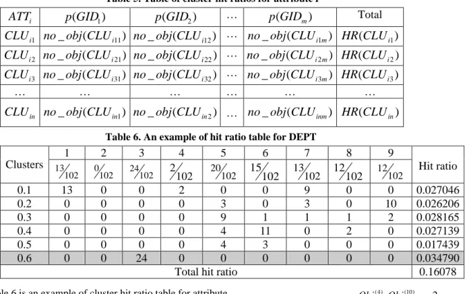
(5) generate result equivalence classes (1). GID=1 ⇒ X1={Obj(2),Obj(4),Obj(10),Obj(19)}. generate cause equivalence classes (2). A11 ⇒ DEPT=0.1, A11*={f }, A12 ⇒ DEPT=0.2, A12*={f }, …. all result equivalence classes finished?. A15 ⇒ DEPT=0.6,. no. A15*={Obj(2),Obj(4),Obj(5),Obj(9),Obj(10),Obj(11)}, … A25 ⇒ AMT=0.12, A25*={Obj(4), Obj(10),Obj(15)}, …. create lower approximation rules (3) create upper approximation rules and compute confidence (4) yes yes. delete object of the devised rules (5). no. create new combinatorial rules (6). (b) Compute confidence for upper approximation rules Use equation (3) to compute each rule’s confidence. Here we can assign a threshold value (minimum confidence) to determine which rules are acceptable. For instance,. all cause equivalence classes finished?. CF ( A16 ) = ( *. Obj( 2) , Obj ( 4 ) , Obj(10) 3 )= Obj , Obj ( 4 ) , Obj(5) , Obj (9) , Obj (10) , Obj(11) 6 ( 2). Rules generation completed. “Insert this into the upper rule table as R3: IF dept = 0.06 Then GID = 1 with CF= 1/2.” Figure 5. Flow chart of implementing Rough set. CF ( A25 ) = ( *. Table 4. Example of the cause equivalence classes. Ai , j i. j. DEPT. 0.1. Yi , j YDEPT , 0.1 = {Obj ( 6 ) , Obj ( 7 ) , Obj (12 ) , Obj (13) , Obj (14 ) , Obj (15) , Obj (18 ) }. DEPT. 0.2. YDEPT ,0.2 = {Obj. DEPT. 0.3. YDEPT , 0.3 = {Obj (1) , Obj ( 3) }. DEPT. 0.4. YDEPT , 0.4 = {Obj (8) , Obj (16) }. DEPT. 0.6. AMT. 0. AMT. (17 ). }. YDEPT ,0.6 = {Obj ( 2 ) , Obj ( 4) , Obj ( 5) , Obj (9 ) , Obj (10) , Obj (11) }. 2 Obj ( 4) , Obj(10) )= ( 4) (10 ) (15) 3 Obj , Obj , Obj. “Insert this into the upper rule table as R4: IF amt = 0.12 Then GID = 1 with CF=2/3.” (5) Create new combinatorial rules Following the above procedure we can find single attribute association rules. Sometimes relationships exist between two or more attributes. In the following we consider two or more attributes to generate association rules. But how to combine and what attributes suits to be combined are quite challenging. To solve those questions, we apply a probability model for each cluster. Table 5 is the table of cluster hit ratios. Where. p (GIDl ) : The probability of group l, l ∈ [1, m] , no _ obj (GIDl ) , total _# _ of _ objects. Y AMT , 0 = {Obj (3) }. p (GIDl ) =. 0.02. Y AMT ,0.02 = {Obj (1) }. no _ obj (GIDl ) : The number of objects in group l,. AMT. 0.04. Y AMT , 0.04 = {Obj ( 9) }. ATTi : The attribute i.,. AMT. 0.08. Y AMT , 0.08 = {Obj (5) }. th CLU ij : For attribute i, the j cluster, j ∈ [1, n] ,. AMT. 0.12. Y AMT , 0.12 = {Obj ( 4) , Obj (10) , Obj (15) }. no _ obj (CLU ijl ) : The number of objects for attributes i,. …. …. the jth cluster, in group l,, …. confidences. (a) Create upper approximation rules For example for. th HR (CLU ij ) : The hit ratio of attributes i, the j cluster. m. HR(CLU ij ) = ∑ [−(. no _ obj (CLU ijl ). ) total _# _ of _ objects no _ obj (CLU ijl ) * log( ) * p (GIDl )] total _# _ of _ objects l =1.

(6) Table 5. Table of cluster hit ratios for attribute I. … p(GID1 ) p(GID2 ) no _ obj (CLU i11 ) no _ obj(CLU i12 ) …. no _ obj (CLU i1m ) HR (CLU i1 ). CLU i 2 no _ obj (CLU i 21 ) no _ obj(CLU i 22 ) …. no _ obj (CLU i 2m ) HR(CLU i 2 ). CLU i 3 no _ obj (CLU i 31 ) no _ obj (CLU i 32 ) …. no _ obj (CLU i 3m ) HR(CLU i 3 ). ATTi CLU i1. …. …. …. …. CLU in no _ obj (CLU in1 ) no _ obj (CLU in 2 ) …. Total. p (GIDm ). …. …. no _ obj (CLU inm ) HR(CLU in ). Table 6. An example of hit ratio table for DEPT. 1 Clusters. 13. 0.1 0.2 0.3 0.4 0.5 0.6. 102. 13 0 0 0 0 0. 2 0. 102. 0 0 0 0 0 0. 3 24. 102. 0 0 0 0 0 24. 4 2. 5 20. 102 102 2 0 0 3 0 9 0 4 0 4 0 0 Total hit ratio. Table 6 is an example of cluster hit ratio table for attribute DEPT. Take on for example in Table 6, the hit ratio for cluster DEPT=0.1 is calculated as follows: 13 13 13 HR(DEPT = 0.1) = [−( ) * log( ) * ( )] + 102 102 102 2 2 2 9 9 13 [−( ) * log( ) * ( )] + [−( ) * log( ) * ( )] = 0.02704 102 102 102 102 102 102. Attribute DEPT has a total hit ratio of 0.16078 that indicates the importance level of DEPT. The cluster DEPT = 0.1 has an importance level of 0.027046. We can combine those attributes of various clusters with higher importance levels to find combinatorial rules. User can simply give a threshold of hit ratio to decide what attributes need to be combined for consideration. After computing all the attributes of various clusters with higher hit ratios, we can combine upper approximation rules with higher hit ratio equivalence classes. For instance, in step 5 we have found an upper rule: * A25 ⇒ AMT = 0.12, YAMT ,0.12 = {Obj( 4) , Obj(10) , Obj(15) } We combine them with all attributes which with higher hit ratios. For example, attribute DEPT, where DEPT = 0.6 has higher hit ratios so we combine them. A15 ⇒ DEPT = 0.6, Y DEPT ,0.6 = {Obj ( 2 ) , Obj ( 4 ) , Obj ( 5) , Obj (9 ) , Obj (10) , Obj (11) }. COM ( A 25 , A15 ) ⇒ ( AMT = 0 .12 ) ∩ ( DEPT = 0 .6 ), *. *. (Y AMT ,0.12 ) ∩ (YDEPT ,0.6 ) = {Obj ( 4) , Obj (10) }. 6. 15. 102 0 0 1 11 3 0. 7 13 102 9 3 1 0 0 0. 8 12. 102 0 0 1 2 0 0. CF (COM ( A25 , A15 )) = ( *. *. 9 12. Hit ratio 102. 0 10 2 0 0 0. 0.027046 0.026206 0.028165 0.027139 0.017439 0.034790 0.16078. Obj ( 4) , Obj (10 ) 2 )= ( 4) (10 ) 2 Obj , Obj. “Insert this into the variation rule table as R5: IF amt = 0.12 and dept=0.6 Then GID = 1 CF=2/2.” (6) Go back to (4) until all of the cause equivalence classes are completed. (7) Go back to (3) until all of the result equivalence classes are completed.. 2.4 Step 4-Knowledge Base We summarize and store rules in lower rule table, upper rule table and variation rule table into knowledge base. Those rules can help managers make better decisions and find some unknown patterns in the database that are meaningful for them. Table 7 presents the rules found in the data mining example. For instance, rules 1 to 3 mean that if customers buy products from the store and the total amt levels are 0.04 or 0.08 or 0.22, respectively, then the purchase records or customers belong to cluster 1. These rules have 100 % confidence. Rules 17 and 18 mean that if customers buy products and the total amt level is 0.14 and the department is 0.4, respectively, then they belong.

(7) Table 7. Rules found in example Group 1: R1: amt=0.04, CF= 1.00 R14: amt=0.12, CF= 0.67 R2: amt=0.08, CF= 1.00 R15: amt=0.18, CF= 0.50 R3: amt=0.22, CF= 1.00 R16: dept=0.60, CF= 0.43 Group 2: R4: amt=0.00, CF= 1.00 R17: amt=0.14, CF= 0.50 R5: amt=0.02, CF=1.00 R18: dept=0.40, CF= 0.50 R6: dept=0.3, CF=1.00 … … …. Figure 7. Rough set analysis Here we set threshold equal to 0.2. We discovered 36 lower rule, 26 upper rule and 5 variation rule. For example, Lower rules: If amt = 0.24 or large_no = 0.1 or price = 0.24 then GID=3 (CF=1). Upper rules: If amt = 0.11 or customer =0.4 or price = 0.11 then GID=3 (CF>=0.5). Variation rules: If dept = 0.2 and amt = 0.3 then GID = 3 (CF=0.29). Then we recuperate each attribute back to its original value. Total amount in range 0.24 means: Figure 6. Self-Organization Mapping to cluster 2. These rules have 0.5% confidence. 3.. Results and Discussions. We follow the proposed data mining procedure and conduct data mining on purchase records of a store. Here we select one day of sales volume in a department store. There are 10,123 records in it and approximately memory is 1MB. First we choose sales table and amt, customer, department, product number (good_no), kind of products (Large_no), price and quality. And then we randomly sample one percept of all the 10,123 records from database and transform those data. After normalizing data we proceed to data mining step – SOM and rough set. Here we set radius equal to 5.0 and learning rate equal to 1.0. The change rate of radius and learning rate are both equal to 0.98. The lowest radius and learning rate are 0.01.When the error rate is lower than 0.1, network is then converged. Figure 6 shows the result of SOM. After the network converges we gain the final weights. Then we can compute the final score of each record with final weights. According to the final score we assign each record to its cluster. After SOM, we use rough set to generate association rules that explain what each cluster means. We create result equivalence classes, create lower approximation rules, create upper approximation rules, compute confidence, and create variation rules (Figure 7).. (value − min(amt )) = 0.24 , where max amount = (max(amt ) − min(amt )) 10,600 and min amount = 2. So current amount = $2,523.. We transfer upper rules to explain what cluster 3 means: total amount approximation is equal to 2,000,the kind of product is from 10 to 20, and the price of product approximation is equal to 1,000. Confidences of those characters equal 100%. And total amount approximation equal to 1,000, the kind of customer belongs to 4 and the price of product approximation is equal to 1,000. Confidences of those characters are more then 50%. 4.. Conclusions. In this paper we use two methods to assist our proposed data mining procedure: a neural network –SOM and rough set to discover association rules. SOM clusters the transaction records for data mining preprocess purpose. Rough set theory is used to analyze what each cluster means and what relationships exist between attributes, so as to discovery enterprise rules. These rules can help managers make better decisions, for each cluster by employing corresponding strategy that realizes one by one on-line marketing. Using the proposed data mining system can help discover many of the enterprise rules. But there is still room for improvement. Future challenges include how to cluster customers and products meaningfully, and how to choose training set properly?.

(8) How to evaluate the rules’ appropriately? Besides, in order to make system applicable, domain expertise is usually needed. Therefore, more intelligent systems will be the main focus of our future work.. 5. REFERENCES [1] Agrawal, R., Imielinski, T. and Swami, A., “Mining Association between Sets of Items in Massive Database,” In Proc. Of the ACM-SIGMOD Int’l Conf. On Management of Data, pp. 207-216, 1993. [2] Agrawal, R. and Srikant, R., “Fast algorithms for mining association rules,” In Proc. Of the International Conf. On Very Large Data Bases, pp. 407-419, 1995. [3] Apte, C. and Hong, S.J., “Predicting equity returns from securities data and minimal rule generation,” Advances in Knowledge Discovery (AAAI Press, Menlo Park, CA/ MIT Press, Cambridge, MA), pp. 541-560, 1995. [4] Basu, A., “Theory and Methodology Perspectives on operations research in data and knowledge management,“ European Journal of Operational Research, Vol. 111, pp. 1-14, 1998. [5] Bayardo, R.J., “Efficiently Mining Long Patterns from Databases,” In Proc. Of the ACM-SIGKDD Int’l Conf. On Management of Data, pp. 85-93, 1998. [6] Bayardo, R.J. and Agrawal, R., “Mining the Most Interesting Rules,” In Proc. Of the Fifth ACM-SIGKDD Int’l Conf. On Knowledge Discovery and Data Mining, pp. 145-154, 1999. [7] Bayardo, R.J., Agrawal, R. and Gunopulos, D., “Constriaint-Based Rule Mining in Large, Dense Databases,” In Proc. Of the 15th Int’l Conf. On Data Engineering, pp. 188-197, 1999. [8] Beery, J. A. and Linoff, G., Data mining techniques: for marketing, sales, and customer support, New York: Wiley, 1997. [9] Chen, M.S., “Using Multi-Attribute Predicates for Mining Classification Rules,” IEEE, pp. 636-641, 1998. [10] Deogun, S., Raghavan, V., Sarkar, A. and Sever, H., “Data Mining: Trends in Research and Development,” Rough Sets and Data Mining – Analysis of Imprecise Data, Kluwer Academic Publishers, 1997. [11] Flexer, A., “On the Use of Self-Organizing Mpas for Clustering and Visualization,” In Proc. Of the 3rd Int’l European Conf. PKDD 99, Prague, Czech Republic, 1999. [12] Ha, S.H. and Park, S.C., “Application of data mining tools to hotel data mart on the Intranet for data base marketing,” Expert Systems with Applications, Vol. 15, pp. 1-31, 1998. [13] Han, J. and Fu, Y., “Mining multiple-level association rules in large databases,” IEEE Transactions on knowledge and data engineering, Vol. 11, No.5, pp. 798-804, 1999. [14] Houtsma, M. and Swami, A., “Set-oriented mining of association rules,” Research Report RJ 9567, IBM Almaden Research Center, San Jose, California, 1993. [15] Kleissner, C., “Data Mining for the Enterprise,” In Proc. Of the 31st Annual Hawaii International Conf. On System Sciences, pp. 295-304, 1998.. [16] Lin, T.Y. and Cercone, N., Rough Sets and Data Mining – Analysis of Imprecise Data, Kluwer Academic Publishers, 1997. [17] Mastsuzawa, H. and Fukuda, T., “Mining Structured Association Patterns from Databases,” In Proc. Of the 4th Pacific-Asia Conference, PAKDD 2000, Kyoto, Japan, pp. 233-244, 2000. [18] Pasquier, N., Bastide Y., Taouil, R. and Lakhal, L., “Efficient mining of association rules using closed itemset lattices,” Information system, Vol. 24, No. 1, pp. 25-46, 1999. [19] Toivonen, H., Klemettinen, M., Ronkainen, P., Hatonen, K. and Mannila, H., “Pruning and grouping of discovered association rules,” In Workshop Notes of the ECML95 Workshop on Statistics, Machine Learning, and Knowledge Discovery in Databases, pp. 47-52, 1995. [20] Tsechansky, S., Pliskin, N., Rabinowitz, G. and Porath, A., “Mining relational patterns from multiple relational tables,” Decision Support Systems, Vol. 27, pp. 177-195, 1999. [21] Tsur, D., Ullman, J.D., Abiteboul, S., Clifton, C., Motwani, R. Nestorov, S. and Rozenthal, A., “Query flocks: A generalization of association –rule mining,” In Proc. Of the ACM-SIGMOD, pp. 1-12, 1998. [22] Zhang, T., “Association Rules,” In Proc. Of the 4th Pacific-Asia Conference, PAKDD 2000, Kyoto, Japan, pp. 233-244, 2000..

(9)