音樂節奏特性與心率變異性之關聯性研究及其硬體實現

全文

(1)國立交通大學電機與控制工程學系碩士論文. 音樂節奏特性與心率變異性之關聯性研究及其硬體實現. A Study of the Relationship between Two Musical Rhythmic Characteristics and Heart Rate Variability (HRV) with Hardware Implementation for HRV analysis. 研究生:林士翔指導教授:黃聖傑中華民國九十七年六月.

(2) 音樂節奏特性與心率變異性之關聯性研究及其硬體實現 A Study of the Relationship between Two Musical Rhythmic Characteristics and Heart Rate Variability (HRV) with Hardware Implementation for HRV analysis. 研究生：林士翔. Student：Shih-Hsiang Lin. 指導教授：黃聖傑. Advisor：Sheng-Chieh Huang. 國立交通大學電機與控制工程學系碩士論文. A Thesis Submitted to Department of Electrical and Control Engineering College of Electrical and Computer Engineering National Chiao Tung University in partial Fulfillment of the Requirements for the Degree of Master in Electrical and Control Engineering June 2008 Hsinchu, Taiwan, Republic of China. 中華民國九十七年六月.

(3) 音樂節奏特性與心率變異性之關連性研究及其硬體實現. 學生：林士翔. 指導教授：黃聖傑國立交通大學電機與控制工程學系碩士班. 摘要. 心率變異性源自心臟搏動速率隨時間不斷的在變化。這種不斷變異的現象主要受人體自主神經系統所控制。在過去二十幾年的研究當中，心率變異性分析已成為越來越普遍的自主神經系統功能性指標。而日常生活中舉凡各種內臟功能、血壓、情緒變化乃至生活壓力等等…，都和自主神經系統的調節息息相關。因此本研究以心率變異性為生理觀測指標，觀察不同節奏特性之音樂所造成的自主神經系統調變情形。本研究基於音樂感知、音訊處理和心電訊號分析提出音樂的兩大節奏特性（節拍速度和節奏複雜度）調變心率變異性之假設。並由實驗結果發現，擁有節拍速度較快且複雜度較低之特性的節奏樣本，有較明顯的同步能力。所謂同步能力即音樂節奏促使心跳節奏產生改變並趨於相似之特性。此外在聆聽完此種特性之節奏樣本後，交感神經系統與副交感神經系統活性之比值的下降情形最為顯著，達到一種甚至比平常休息時更為放鬆的生理狀態。在硬體實做方面，本研究在精確度損失極少的前提下，針對所採用之 QRS 波偵測演算法進行部分簡化以減少硬體設計之複雜度，並透過心電圖標準資料庫的驗證，實現高準確率且低成本的 QRS 波偵測晶片。透過系統化的研究方法，了解各種不同特性的音樂對人體自主神經系統造成的影響，以期藉由音樂調節身心，讓生活更加健康。. i.

(4) A Study of the Relationship between Two Musical Rhythmic Characteristics and Heart Rate Variability (HRV) with Hardware Implementation for HRV analysis. Student: Shih-Hsiang Lin. Advisor: Sheng-Chieh Huang. Department of Electrical and Control Engineering National Chiao Tung University. Abstract Heart rate variability (HRV) is a measure of variations in the heat rate. Over the last 25 years, HRV analysis has became more and more popular as a non-invasive research and clinical tool for indirectly investigating both cardiac and autonomic nervous system (ANS) function in both health and disease area. It is choused as the physiological indicator for observing musical effect on ANS modulation. In this study, the concept of two musical rhythmic features, tempo and complexity, modulating human ANS is proposed. The main findings in this work are as follows. The rhythm pattern with faster tempo and lower complexity is observed to decrease the LF/HF and SDNN measure significantly in the resting period after the loop listening rather than the stable resting state. In the hardware implementation part, a high accuracy and low cost QRS detector SoC is realized. By understanding the relationship between music and the function of ANS, we can improve our life and health by music – non-invasively and simply.. ii.

(5) 誌謝終於，我完成了人生第一本論文。回想起這三年的研究生活，有歡樂、有淚水、有感動、更少不了挫折。在專注完美近乎苛求的研究環境下，讓我不斷茁壯成長。比起剛考上研究所那個稚嫩的我，現在顯得更充滿自信和對人生的期許。研究這條佈滿荊棘的路上，那些支持我、鼓勵我、建議我和不吝訓斥我的人，我都由衷的感激你們。沒有你們，這條路將無比漫長，沒有你們，也許半途中我已傷痕累累的倒下了！首先，要感謝當初願意收我的實驗室大家長－黃聖傑老師。在老師以『人』為出發點的科技思維引領之下，讓我找到了自己感興趣的研究主題，促成了這個論文主題的誕生。實驗室在老師的帶領下呈現自由開放且自主學習的環境，讓我們有探索興趣的機會，也養成了自我督促的習慣，非常慶幸自己可以在這樣的環境當中學習成長，謝謝老師！接著，要感謝在我口試的時候，詹明宜老師、邱一老師、蔡宗漢老師和蕭如宣老師，不辭辛勞來評鑑及指導我的研究成果，給予我寶貴的意見讓論文得以更加完整。在研究期間曾多次向詹明宜老師請益，由於跨領域的思維陌生，詹老師總能以過來人的經驗給予我極度中肯的意見和殷切的鼓勵，實在是我研究旅程上的一盞明燈。碩士一年級的時候也曾受蕭如宣老師指導電路版製作流程，著實獲益匪淺。再來，要感謝實驗室一同打拼的伙伴們，煜傑，感謝你從龍騰微笑競賽贏回來的 21 吋LCD，讓我從事研究的時候事半功倍，也從你身上學到了實事求是的精神，我不會忘記 15 天的德國之旅。清彥，感謝你的外線總是可以給我適時的火力支援，讓我籃板沒有白搶，你井然有序的精神不僅體現在你的晶片設計上，也體現在你總是超級整潔的桌面上。雷峻學長，感謝你在我口試前提出的許多中肯的建議，讓口試更加順利圓滿。奕澄學長，感謝你在醫學領域上的專業知識，和你一同討論許多難題總能迎刃而解。還有 Marcel學長、有梁學長、哲明學弟，在meeting的時候你們猛烈的砲火都成了這本論文的血淚。另外，還有簡韶義老師和其實驗室的同學們，一起meeting的時候提出許多很好的建議，也讓我接觸到許多不同領域的研究。當然還要感謝那些填滿我除了埋首案牘以外時光的朋友們。泳隊的伙伴們，永遠不會忘記在我靈感盡失、全身疲軟的時候，你們用綿綿不絕的水花來迎接我，在泳池的嘻笑時光讓我忘卻煩憂。大學的室友，士傑、忠諺、明翰，研究路上彼此打氣。還有非常厲害的子德，在硬體實現的部分幫了我不少忙。感謝開心果，繹心，在一起的時光體驗了許多新鮮事。遭受委屈的時候你能讓我破涕為笑，得意忘形的時候你提醒我居安思危，在口試前一晚的演練，你不厭煩的熬夜當 iii.

(6) 聽眾，給我許多珍貴的建議，謝謝你在這一路上的陪伴。最後，我要感謝我的爸爸、媽媽和妹妹，你們是研究上的最強支柱，讓我可以無後顧之憂的專注向前，你們的行事作風也如春風化雨般的影響著我，沒有你們就沒有今天的我。再一次感謝那些曾經幫助過我、支持我的許多人，因為有你們，我才能完成這本論文，謝謝大家。. iv.

(7) Contents 1. 2. Introduction ........................................................................................................................ 1. 1.1. Motivation ..........................................................................................................1. 1.2. Goal ....................................................................................................................3. 1.3. The Relating Works and Our Innovation............................................................3. 1.4. Application .........................................................................................................5. 1.5. Thesis Organization............................................................................................5. Background ......................................................................................................................... 6. 2.1. Physiology Background...........................................................................................6 2.1.1 Introduction of Electrocardiogram ....................................................................6 2.1.2 Definition of Electrocardiography Configurations..........................................10 2.1.3 Determining Heart Rate from the Electrocardiogram ..................................... 11 2.1.4 Heart Rate Variability ...................................................................................... 11 2.1.5 Physiological Correlates of Heart Rate Variability..........................................12. 2.2 3. Heart’s Hearing......................................................................................................13. Approach ........................................................................................................................... 15. 3.1. HRV Signal Processing Flow ................................................................................15 3.1.1 Acquirement of the ECG signals .....................................................................15 3.1.2 QRS detection..................................................................................................16 3.1.3 Evaluating the QRS detection algorithm .........................................................24 3.1.4 Abnormal Beats Rejection and Compensation ................................................25 3.1.5 Interpolation and De-trending .........................................................................28 3.1.5.1 Interpolation .........................................................................................28 3.1.5.2 Detrending ............................................................................................31 3.1.6 Measures of Heart Rate Variability .................................................................33 3.1.6.1 Time domain measures .........................................................................33 3.1.6.2 Frequency domain measures ................................................................34. 3.2. Drum loop rhythmic analysis ................................................................................36 v.

(8) 3.2.1 Tempo ..............................................................................................................37 3.2.2 Complexity ......................................................................................................39 3.3. Arrangement of Experiment ..................................................................................39 3.3.1 Subject and Environment ................................................................................39 3.3.2 Music Stimuli ..................................................................................................40 3.3.1 Study Protocol .................................................................................................41. 4. 5. 6. Experimental Results ....................................................................................................... 43. 4.1. Data Presentation..............................................................................................43. 4.2. Main Finding ....................................................................................................43. Implementation ................................................................................................................. 53. 5.1. Motivation of HRV Chip .......................................................................................53. 5.2. Accuracy Simulation .............................................................................................54. 5.3. Hardware Architecture...........................................................................................54. 5.3. The Specs...............................................................................................................57. Conclusion ......................................................................................................................... 59. 6.1. Discussion..............................................................................................................59. 6.2. Conclusion.............................................................................................................62. 6.3. Future Work ...........................................................................................................63. Bibliography ............................................................................................................................ 66 Appendix A ..............................................................................................................................72 Appendix B ..............................................................................................................................76 Appendix C..............................................................................................................................78. vi.

(9) List of Tables Table 3.1: The performance of simplified algorithm adopted in this work ..............................25 Table 3.2: The HRV measures of time and frequency domain analysis ...................................35 Table 3.3: Two rhythmic characteristics of the four testing drum loop samples......................41 Table 4.1: The numerical expression of two notable findings in the experimental results ......45 Table 5.1: Summary of the high accuracy QRS detector SoC..................................................57 Table 5.2: Comparison of HRV analysis SoC...........................................................................58 Table A.1: PhysioBank Annotations.........................................................................................72 Table A.2: The evaluation results of the simplified QRS detector ...........................................73 Table C.1: The detailed deviation between the hardware and software QRS detector of each record........................................................................................................................................78. vii.

(10) List of Figures Fig. 1.1: Human-Based Intelligent Music Playing System ........................................................2 Fig. 2.1: Electrocardiogram ........................................................................................................7 Fig. 2.2: Relationship of current flow to lead axis and electrocardiogram deflection ...............7 Fig. 2.3: The standard ECG leads...............................................................................................8 Fig. 2.4: (a) A complete cardiac cycle. (b) Membrane resting potential of cardiac cell.............8 Fig. 2.5: The variation of membrane potential in a complete contraction and relaxation cycle 8 Fig. 2.6: The normal sequence of cardiac depolarization and repolarization and derivation of ECG ............................................................................................................................................9 Fig. 2.7: A typical ECG tracing ................................................................................................10 Fig. 2.8: Four numbered QRS complex waves.........................................................................10 Fig. 2.9: The time series of beat-to-beat intervals .................................................................... 11 Fig. 2.10: The spectral analysis of HRV. ..................................................................................12 Fig. 3.1: The block diagram of the overall signal processing flow of HRV analysis ...............15 Fig. 3.2(a): MSI E3-80 .............................................................................................................16 Fig. 3.2(b): Electrodes placement.............................................................................................16 Fig. 3.3: Relative power spectra of QRS complex, P and T waves, muscle noise and motion artifacts based on an average of 150 beats ...............................................................................17 Fig. 3.4: QRS peak detection flow ...........................................................................................18 Fig. 3.5: Results of each step of Fig. 3.4 ..................................................................................18 Fig. 3.6(a): Amplitude response of the low-pass filter .............................................................19 Fig. 3.6(b): Phase response of the low-pass filter ....................................................................19 Fig. 3.7(a): Amplitude response of the high-pass filter ............................................................20 Fig. 3.7(b): Phase response of the high-pass filter ...................................................................20 Fig. 3.8: Amplitude response of band-pass filter composed of low-pass and high-pass filters21 Fig. 3.9(a): Amplitude response of the derivative ....................................................................22 Fig. 3.9(b): Phase response of the derivative ...........................................................................22 Fig. 3.10: The corresponding relation between ECG raw data and the signals after moving viii.

(11) window average........................................................................................................................24 Fig. 3.11(a) Abnormal beats detection......................................................................................27 Fig. 3.11(b) Abnormal beats removement and compensation ..................................................27 Fig. 3.12: The RR interval time series after 4Hz cubic spline interpolation. ...........................28 Fig. 3.13: The fundamental idea behind cubic spline interpolation .........................................29 Fig. 3.14: The RR interval time series after de-trending. .........................................................31 Fig. 3.15: Time-varying frequency response of L ( N − 1 = 50 and λ = 10 ) . Only the first half of the frequency response is presented, since the other half is identical ..................................32 Fig. 3.16 Frequency responses, obtained from the middle row of L , for λ = 1, 2, 4, 10, 20, 50, and 300. The corresponding cutoff frequencies are 0.189, 0.132, 0.093, 0.059, 0.041, 0.025, and 0.011 times the sampling frequency ..................................................................................33 Fig. 3.17(a): The sound wave of one single note......................................................................37 Fig. 3.17(b): Onset, attack and transient...................................................................................37 Fig. 3.18: Flowchart of a standard onset detection algorithm ..................................................38 Fig. 3.19: The rhythmic characteristics, tempo and complexity, of the four drum loop patterns ..................................................................................................................................................40 Fig. 3.20: The overall experimental flow of one trial...............................................................41 Fig 3.21: The experiment manual.............................................................................................42 Fig. 4.1: The C2 comparison of LF/HF measure......................................................................44 Fig. 4.2: The C2 comparison of SDNN measure......................................................................45 Fig. 4.3: The C1 comparison of SDNN measure......................................................................45 Fig. 4.4: The C1 and C2 comparisons of LF/HF measure........................................................46 Fig. 4.5: The C1 and C2 comparisons of SDNN measure........................................................47 Fig. 4.6: The C1 and C2 comparisons of THB measure...........................................................48 Fig. 4.7: The C1 and C2 comparisons of MRR measure..........................................................49 Fig. 4.8: The C1 and C2 comparisons of RMSSD measure .....................................................50 Fig. 4.9: The C1 and C2 comparisons of LF measure..............................................................51 Fig. 4.10: The C1 and C2 comparisons of HF measure ...........................................................52 Fig. 5.1: The bit-width of each processing block .....................................................................53 Fig. 5.2: The deviation of detected R peak between the software QRS detector and the hardware QRS detector.............................................................................................................54 Fig. 5.3: The systolic array architecture for digital filters ........................................................55 ix.

(12) Fig. 5.4 The connecting array architecture of QRS detection preprocessing stage..................56 Fig. 5.5: The proposed PE reusing architecture........................................................................56 Fig. 5.6: The layout of the high accuracy QRS detector chip ..................................................58 Fig. 6.1: (a) The C1 comparison of LF/HF measure (b) The C2 comparison of LF/HF measure ..................................................................................................................................................59 Fig. 6.2: The Wundt curve for the relation between music complexity and preference...........60 Fig. 6.3: The inverted U-shaped curve for the relation between the surprising factor and rhythmic complexity.................................................................................................................61 Fig. 6.4: (a) The C1 comparison of SDNN measure (b) The C2 comparison of SDNN measure ..................................................................................................................................................61 Fig. 6.5: A systematic model which links music perception and relating physiological responses...................................................................................................................................63. x.

(13) Chapter 1 Introduction 1.1. Motivation The heartbeat interval in humans is known to exhibit fluctuation which is refereed to as. heart rate variability (HRV). The clinical relevance of heart rate variability was first noted by Hon and Lee [1]. They discovered the fetal distress was preceded by alternations in heartbeat intervals before any appreciable change occurred in the heart rate itself. HRV has received a tremendous amount of attention since the seminal work of Akselrod et al. [2]. Established clinical applications of HRV include risk assessment of patients after myocardial infarction and early diagnosis of diabetic autonomic neuropathy [3]. The past researches have witnessed a significant relationship between the autonomic nervous system and cardiovascular mortality, including sudden cardiac death. HRV represents one of the most promising markers. The easy derivation of this measure has popularized its use. Our emotion and physiological state can be modulated by listening to different music. A variety of studies have reported the musical effect on human psychological and physiological states. Through the nervous control mechanisms, a neural coupling into the cardiac canters of the brain, it is possible to vary the heart rate of human subjects non- invasively by causing an entrainment of the sinus rhythm with external auditory stimuli [4]. Although cardiac automaticity is intrinsic to various pacemaker tissues, heart rate and heart rhythm are largely under the control of the autonomic nervous system [5]. The autonomic nervous system (ANS) is the part of the peripheral nervous system that 1.

(14) acts as a control system, maintaining homeostasis in the body. Its main components are its sensory system, motor system (comprised of the parasympathetic nervous system and sympathetic nervous system), and the enteric nervous system. Sympathetic and parasympathetic divisions typically function in opposition to each other. The sympathetic division acts like the accelerator and the parasympathetic division acts like the brake. For example, the sympathetic division accelerates the heart rate in the emergency; while the parasympathetic division decelerates the heart rate in the resting state. Therefore, it can be further inferred that there must be a connection between the musical stimuli and the synergistic action of the autonomic nervous system. It is mentioned that the complex bodily rhythms are ubiquitous in living organisms. These rhythms arise from stochastic, nonlinear biological mechanisms interacting with a fluctuating environment [6]. And experts in the field of music and sound therapy think that there is one major ways in which music and sound can affect our lives. It is called that the principle of entrainment and refers to the phenomena of being in synchronization [7]. It describes a process whereby two rhythmic processes interact with each other in such a way that they adjust towards and eventually ‘lock in’ to a common phase and/or periodicity. For example, we tap foot and shake body to the beat of a song. In other words, our bodies automatically adjust to the pace, rhythm, or pulse of music. And this is why the rhythmic characteristic of music is first considered in this work. Inspired by these previous researches, this study focuses on exploring the relationship between the musical rhythmic characteristics and heart rate variability (a functional indicator of autonomic nervous system).. Fig. 1.1: Human-Based Intelligent Music Playing System 2.

(15) 1.2. Goal Generally, scientific research has four goals: description of behavior, prediction of. behavior, determination of the causes of behavior and explanations of behavior [8]. Mapping to this research, the behavior to be studied in this work is the physiological response induced by the music with different rhythmic characteristics. The heart rate variability (HRV) is taken as the description of behavior. So the goals of this study are listed below: 1. The changes of HRV can be predicted when the subject is listening to music with a specific rhythmic style. 2. Finding the specific features of musical rhythm which dominate the changes of HRV. 3. Explaining how these features results in the changes of HRV. The final dream to be realized is to construct a physiology-based intelligent music playing system shown in Fig. 1.2. The black box named “Core Research” plays the role to link physiological responses and receiving music stimuli and it is what this study wants to explore. What dose the system can do? For example, a user who feels lethargic or depressed might need to listen to some music and get more vigor. First, the system receives the desired physiological or emotional state as input. In this case, being vigorous and energetic is the input of the system. Then, the system can automatically pick some moderate music to play. At the same time, the user’s real-time physiological information feed back to the system. The feedback information not only shows if the automatically choused music works, but also is the basis for advanced learning mechanism. Through network transmitting, the physiological signals are recorded and analyzed in the remote servers. By the long-term machine learning, the system will be highly accurate and personalized for healthcare and goal-driven music listening.. 1.3. The Relating Works and Our Innovation There were some relating works which discuss the physiological responses induced by. music in the past. For example, the previous work discussed the changes in the cardiovascular and respiratory system induced by music, specifically tempo, rhythm, melodic structure, pause, individual preference, habituation, order effect of presentation and previous musical 3.

(16) training [9]. They captured the physiological signals and observed the responses induced by different music. Our innovation is a “systematical” method to study the physiological changes induced by music. Music perception is not straightforward. There are usually several musical elements in one song. For constructing a systematical model, various features of music need to be extracted from a song first. Then, the changes of biomedical signals induced by these specific musical features are studied. How do these changes integrate to the final physiological or emotional modulation is another more complex problem. When discussing the relationship between music and human cardiovascular system, rhythm is thought as the most important music feature because of the principle of entrainment. For excluding other musical features except for rhythm, drum loop music with simple and pure rhythmic characteristic is choused as the musical stimuli samples in this study. The other reason inspires us to focus on the rhythmic characteristics is the similarity between heart rhythm and musical rhythm. It can be imagined that how boring it is that one piece of song composed of monotone and even-spaced beat. It is in the same condition for the heartbeat rhythm. If our heartbeat rhythm follows a regular even a constant rate, it means that our body can’t maintain the equilibrium state through the fluctuations resulted from the interaction between the external or internal environments and physiological control mechanism. One big challenge confronted in this study is how to quantitatively define rhythm. Two musical rhythmic features, tempo and complexity, are proposed to quantitatively describe rhythm. Sound by its very nature is temporal. So the tempo is the first necessary feature to represent the rhythm. The second feature, complexity, is inspired from the observation of similarity between the musical rhythm and human heart rhythm. Both of them are not a constant or invariable pattern. Another consideration to choose drum loop music as the experimental stimulus is to exclude the individual music preferences. The same music maybe results in two kinds of absolutely different feeling (emotion or physiological responses) between you and me. The drum loop music is easier to exclude the individual music preferences because of its simplicity. Besides, the experiment protocol is carefully designed for more stable and trustable results.. 4.

(17) 1.4. Application Some studies have pointed out that the different music can be used to improve our lives,. for example, promoting sleep [10], reducing anxiety [11], assisting exercise [12] and even increasing brain activity [13]. And these daily activities are all closely related to the autonomic nervous system. The HRV is an indicator of the autonomic nervous system. In other words, the effect of music on the mentioned activities can be assessed by HRV. Once the detail of how music affects human was revealed, people can improve life and health by music – non-invasively and simply.. 1.5. Thesis Organization The thesis is divided into six chapters. In chapter 2, Background, I review most relevant. to my research in these fields: “electrophysiology of the heart” and “heart’s hearing”. In chapter 3, Approach, I explain more formally the problem I am trying to solve, the signal processing flow of HRV, the music analysis algorithms and the arrangement of experiment. In chapter 4, Experimental Results, presents the results of experiment and some inferences are given. In chapter 5, Implementation, the hardware architecture design for QRS complex detection is proposed and a high accuracy and low cost QRS detector chip is implemented. Chapter 6, Conclusion, the contributions made in this study and suggesting directions for further work are summarized.. 5.

(18) Chapter 2 Background 2.1. Physiology Background In this section, some basic physiological knowledge related to this study is introduced. and the physiological measurement, heart rate variability (HRV), will be explained in detail.. 2.1.1 Introduction of Electrocardiogram An electrocardiogram (ECG or EKG) shown in Fig. 2.1 is a graphic which records the electrical activity of the heart over time. The sinoatrial node (abbreviated SA node, also called the sinus node) is the electrical impulse generating tissue located in the right atrium of the heart. The electrical impulse from the SA node triggers a sequence of electrical events in the heart to control the orderly sequence of muscle contractions that pump the blood out of the heart. The depolarization and re-polarization of the SA node and the other elements of the heart's electrical system produces a strong pattern of voltage change. The voltage change can be measured with electrodes on the skin. Therefore, the ECG is a starting point for detecting many cardiac problems. It is used routinely in physical examinations and for monitoring the patient's condition during and after surgery, as well as during intensive care. When a string galvanometer was used, an electrical current passed through electrodes connected to two extremities caused deflection of the recording instrument. Passage of current 6.

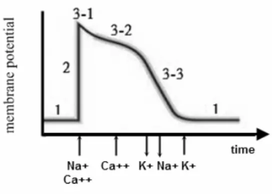
(19) Fig. 2.2: Relationship of current flow to lead Fig. 2.1: Electrocardiogram. axis and electrocardiogram deflection. toward the positive end of a bipolar electrode was set to cause a positive deflection of the recorder shown in Fig. 2.2. The electrodes are traditionally placed on arms and legs for convenience. These connections are called leads. It refers to a combination of electrodes that form an imaginary line in the body along which the electrical signals are measured. The standard leads are shown in Fig. 2.3. There are two main stages of electrical activity in a complete contraction and relaxation cycle of a cardiac cell: polarization and depolarization, as shown in Fig. 2.4(a). The detailed steps in a complete contraction and relaxation cycle are demonstrated as follows.. (1) Polarization In the resting state the membrane resting potential of cardiac cell is about -90mV because of the unbalance of ions as shown in Fig. 2.4(b). The cardiac cells are ready to receive electrical impulses.. (2) Depolarize (polarization to depolarization) When the cardiac cells begin depolarization, the fast sodium channels open and plenty sodium ions flow into the cell. The membrane potential increases sharply.. (3) Repolarize (depolarization to polarization) The process that the membrane potential returns to membrane resting potential is called repolarization. It can be divided into three steps: (3-1) the sodium channels close, (3-2) the calcium ions flow into cell slowly and (3-3) the potassium ions flow out cell. The variations of membrane potential in each step of a complete contraction and relaxation cycle are shown in Fig. 2.5. How the normal sequence of cardiac depolarization and repolarization derivates 7.

(20) the ECG is shown in Fig. 2.6. In the next section, the causes of different wave in the electrocardiogram will be explained.. Fig. 2.3: The standard ECG leads. (a). (b). Fig. 2.4: (a) A complete cardiac cycle. (b) Membrane resting potential of cardiac cell. Fig. 2.5: The variation of membrane potential in a complete contraction and relaxation cycle 8.

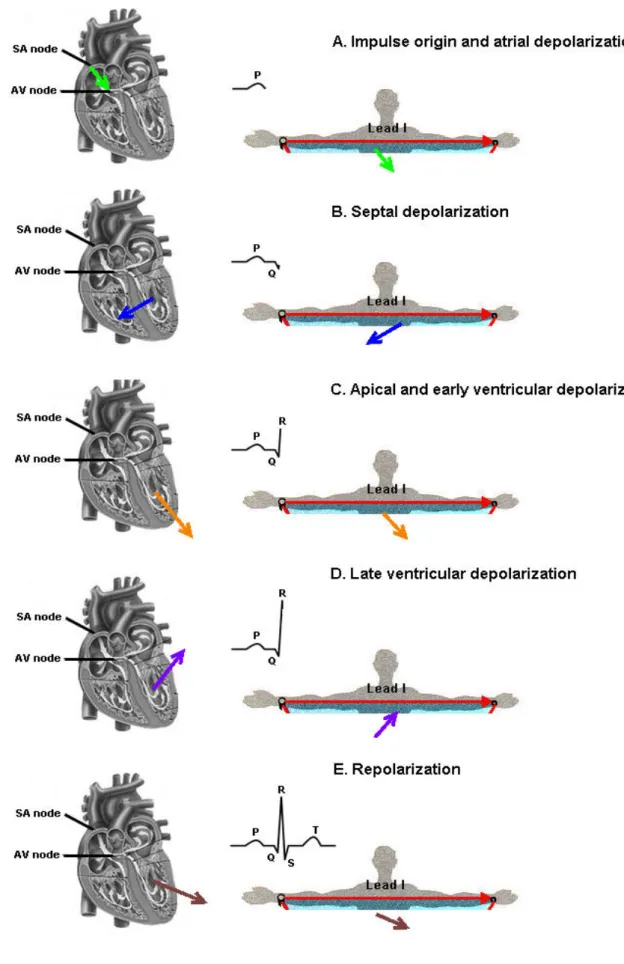
(21) Fig. 2.6: The normal sequence of cardiac depolarization and repolarization and derivation of ECG 9.

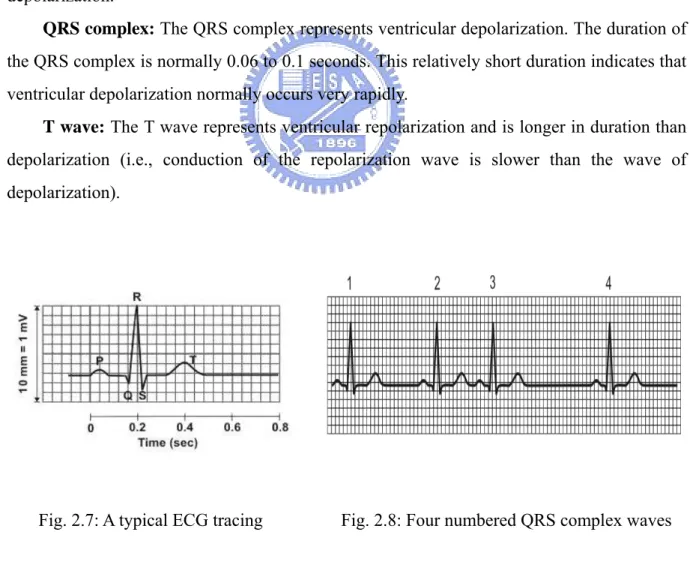
(22) 2.1.2 Definition of Electrocardiography Configurations As the heart undergoes depolarization and repolarization, the electrical currents that are generated spread not only within the heart, but also throughout the body. This electrical activity generated by the heart can be measured by an array of electrodes placed on the body surface. A typical ECG tracing is shown in Fig. 2.7. The different waves that comprise the ECG represent the sequence of depolarization and repolarization of the atria and ventricles. P wave: The P wave represents the wave of depolarization that spreads from the SA node throughout the atria, and is usually 0.08 to 0.1 seconds (80-100 ms) in duration. The period of time from the onset of the P wave to the beginning of the QRS complex is termed the PR interval, which normally ranges from 0.12 to 0.20 seconds in duration. This interval represents the time between the onset of atrial depolarization and the onset of ventricular depolarization. QRS complex: The QRS complex represents ventricular depolarization. The duration of the QRS complex is normally 0.06 to 0.1 seconds. This relatively short duration indicates that ventricular depolarization normally occurs very rapidly. T wave: The T wave represents ventricular repolarization and is longer in duration than depolarization (i.e., conduction of the repolarization wave is slower than the wave of depolarization).. Fig. 2.7: A typical ECG tracing. Fig. 2.8: Four numbered QRS complex waves. 10.

(23) Fig. 2.9: The time series of beat-to-beat intervals. t (n) for n ∈ {1,..., N } I (n + 1) = t (n + 1) − t (n) n ∈ {1,..., N − 1}. ( 2.1 ). 2.1.3 Determining Heart Rate from the Electrocardiogram The term "heart rate" normally refers to the rate of ventricular contractions. As shown in Fig. 2.8, there are four numbered QRS complex waves, each of which is preceded by a P wave. Therefore, the atrial and ventricular rates will be the same because there is a one-to-one correspondence. Atrial rate can be determined by measuring the time intervals between P waves (P-P intervals). Ventricular rate can be determined by measuring the time intervals between the QRS complex waves (R-R intervals).. 2.1.4 Heart Rate Variability Over the last 25 years, HRV analysis has became more and more popular as a non-invasive research and clinical tool for indirectly investigating both cardiac and autonomic nervous system (ANS) function in both health and disease area. The current methodologies used to analyze HRV are based largely on linear techniques to analyze past and present 11.

(24) Fig. 2.10: The spectral analysis of HRV.. electrocardiogram (ECG) data in time and frequency domains. HRV is a measure of variations in the heart rate. It is usually calculated by analyzing the time series of beat-to-beat intervals from the electrocardiogram. As shown in Fig. 2.9, the top curve is a simplified ECG and the corresponding time series of beat-to-beat intervals I(n) is calculated as (2.1) and shown in the bottom. Various measures of heart rate variability are all based on the time series. The variations of these measures after listening to music are expected to be observed and the musical rhythmic effect is discussed in this study.. 2.1.5 Physiological Correlates of Heart Rate Variability Measures of heart rate variability are increasingly being employed in applications ranging from basic investigations of central regulation of autonomic state to studies of fundamental links between psychological processes and physiological functions, to evaluations of cognitive development and clinical risk. As psychological correlates and physiological mechanisms are being delineated, measures of heart rate variability may offer powerful tools for the clarification of relationships between psychological and physiological processes. Although cardiac automaticity is intrinsic to various pacemaker tissues, heart rate and heart rhythm are largely under the control of the autonomic nervous system [14]. An understanding of the modulatory effects of neural mechanisms on the sinus node has been 12.

(25) enhanced by spectral analysis of HRV shown in Fig. 2.10 [2]. Vagal activity is the major contributor to the HF component. Disagreement exists in respect of the LF component. Some studies suggest that LF, when expressed in normalized units, is a quantitative marker for sympathetic modulations, other studies view LF as reflecting both sympathetic and vagal activity. Consequently, the LF/HF ratio is considered by some investigators to mirror sympatho/vagal balance. The origins of heart rate variability are discussed deeply in [15]. There were many researches discussing the relationship between human’s physical state and HRV in the past. The decline in heart rate variation with increasing age was reported in [16]. Endurance exercise increases parasympathetic activity and decreases sympathetic activity in the human heart at rest [17]. The changes of heart rate was used as the parameter to distinguish between positive and negative emotions [18]. The sympathovagal interaction during mental stress was assessed in [19]. Based on these researches, HRV can be taken as an indicator of assessing physical and emotional state. The music modulating effect on human autonomic nervous system can be inferred indirectly from HRV.. 2.2. Heart’s Hearing It is a generally accepted concept that our emotion and physical state change when. listening to different music. For example, Rock music makes someone feel vigorous and increases the heart rate and Jazz music makes someone feel lethargic and slows his breath down. Is there any physiological pathway which links the perception of music with the responses of ANS? Research has revealed that the heart rate can be controlled by external stimuli [4]. However, following several years of research, it was observed that, the heart communicates with the brain in ways that significantly affect how we perceive and react to the world. Neurophysiologists discovered a neural pathway and mechanism whereby input from the heart to the brain could inhibit or facilitate the brain’s electrical activity [20]. From these researches the connection and communication between brain and heart are established. On the other hand, it is long known that changes in emotions are accompanied by predictable changes in physiological state such as heart rate, blood pressure, respiration and digestion. When someone is aroused, his sympathetic division of the autonomic nervous system energizes him for fight or flight. When someone is in quiet times, the parasympathetic 13.

(26) division cools him down. Based on theses researches, it can be sure that there must be some connection between the music perception and the physical responses.. 14.

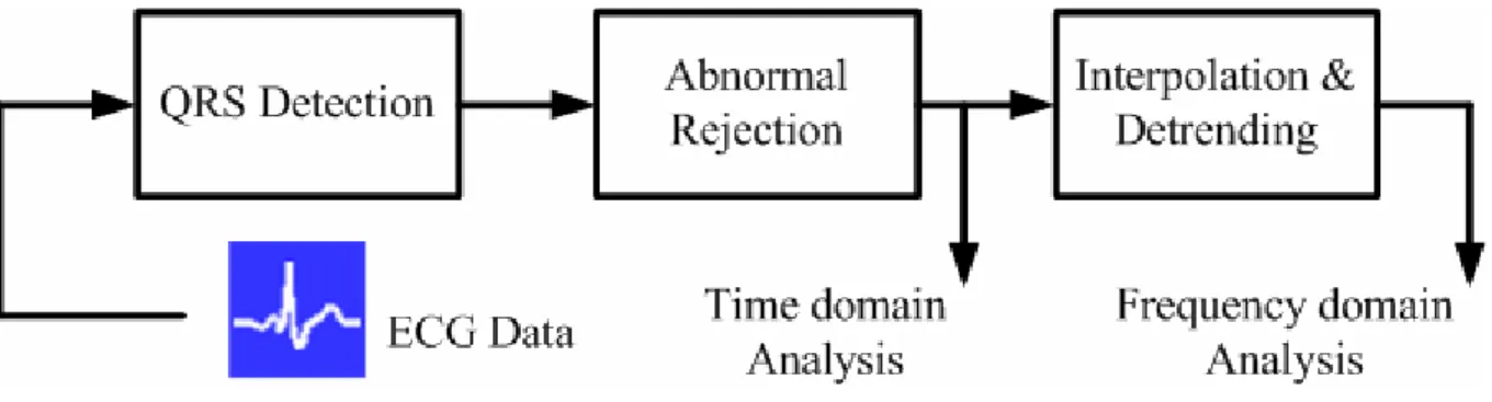
(27) Chapter 3 Approach 3.1. HRV Signal Processing Flow The overall HRV signal processing flow is shown in Fig. 3.1. The processing methods of. each block are detailed in the following subsection.. 3.1.1 Acquirement of the ECG signals The ECG signal is captured by a 3-channel portable device (MSI E3-80, FDA 510(k) K071085) at 500Hz sampling rate from the chest surface of body shown in Fig. 3.2(a) (b) [21]. Only the channel1 (L1) data were taken to be analyzed. In the previous HRV studies, the. Fig. 3.1: The block diagram of the overall signal processing flow of HRV analysis 15.

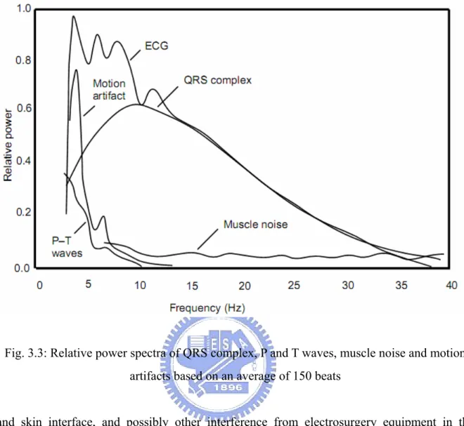
(28) Fig. 3.2(a): MSI E3-80. Fig. 3.2(b): Electrodes placement. duration of recording was dictated by the nature of each investigation. And it is recommended that the recording of approximately 1min is needed to assess the HF components of HRV while approximately 2min are needed to address the LF component [3]. Therefore, 2min duration is taken as the shortest unit to be compared in this study.. 3.1.2 QRS detection As the introduction in 2.1.3, the QRS complex is the most notable waveform within the electrocardiography (ECG). Since it reflects the electrical activity within the heart during the ventricular contraction, the time of its occurrence as well as its shape provides much information about the current state of the heart. Due to its characteristic shape it serves as the basis for the automated determination of the heart rate. Therefore, QRS detection provides the fundamentals for almost all automated ECG analysis algorithms. Within the last decade many new approaches to QRS detection have been proposed; for example, algorithms from the field of artificial neural networks, genetic algorithms, wavelet transforms, filter banks as well as heuristic methods mostly based on nonlinear transforms. The detailed review and comparison of these methods were presented [22]. The detection algorithm described by Hamilton and Tompkins is adopted in this work because of its high reliability and low computational load [23-25]. The ECG waveform contains, in addition to the QRS complex, P and T waves, 60-Hz noise from power line interference, EMG from muscles, motion artifact from the electrode 16.

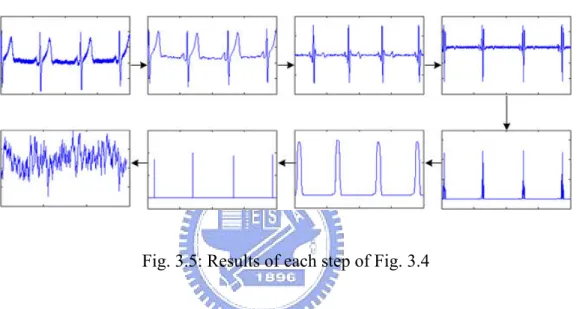
(29) Fig. 3.3: Relative power spectra of QRS complex, P and T waves, muscle noise and motion artifacts based on an average of 150 beats. and skin interface, and possibly other interference from electrosurgery equipment in the operating room. Many clinical instruments such as a cardiotachometer and an arrhythmia monitor require accurate real-time QRS detection. It is necessary to extract the signal of interest, the QRS complex, from the other noise sources such as the P and T waves. Fig. 3.3 summarizes the relative power spectra of the ECG, QRS complexes, P and T waves, motion artifact, and muscle noise based on the previous research [25]. The signal processing flow of QRS detection and the corresponding results are shown in Fig. 3.4 and Fig. 3.5. There are two main stages in the QRS detection flow. One is the preprocessing stage which is composed of various filters for removing noise and acquiring the QRS complex information. The other stage, peak detection, makes use of the information acquired by the preprocessing stage and some criteria to detect the QRS complex peaks. In the beginning of the preprocessing stage, the band-pass filter is used to reduce the influence of muscle noise, 60 Hz interference, baseline wander, and T-wave interference. The desirable pass-band to maximize the QRS energy is approximately 5-15 Hz [25]. 17.

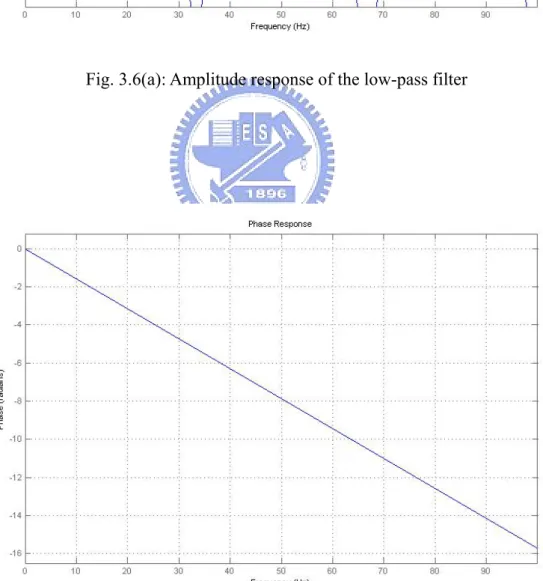
(30) Fig. 3.4: QRS peak detection flow. Fig. 3.5: Results of each step of Fig. 3.4. The band-pass filter is composed of cascaded low-pass and high-pass filters. Their difference equations are listed as (3.1). The performance details of the low-pass filter and high-pass filter are shown in Fig. 3.6 and Fig. 3.7. The amplitude response of the band-pass filter which is composed of the cascade of the low-pass and high-pass filters is shown in Fig. 3.8. The center frequency of the pass-band is at 10 Hz. The amplitude response of this filter is designed to approximate the spectrum of the average QRS complex as illustrated in Figure 12.1. Thus this filter optimally passes the frequencies characteristic of a QRS complex while attenuating lower and higher frequency signals.. LowPass Filter y ( nT ) = 2 y ( nT − T ) − y ( nT − 2T ) + x ( nT ) − 2 x ( nT − 6T ) + x ( nT − 12T ). (3.1) HighPass Filter y ( nT ) = x ( nT − 16T ) −. 1 ⎡ y ( nT − T ) + x ( nT ) − x ( nT − 32T ) ⎤⎦ 32 ⎣ 18.

(31) Fig. 3.6(a): Amplitude response of the low-pass filter. Fig. 3.6(b): Phase response of the low-pass filter. 19.

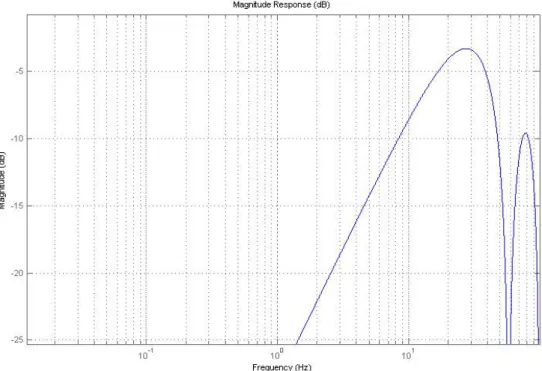
(32) Fig. 3.7(a): Amplitude response of the high-pass filter. Fig. 3.7(b): Phase response of the high-pass filter. 20.

(33) Fig. 3.8: Amplitude response of band-pass filter composed of low-pass and high-pass filters. After the signal has been filtered, it is then differentiated to provide information about the slope of the QRS complex. This derivative is implemented with the difference equation (3.2). The performance characteristics of this derivative implementation are shown as Fig. 3.9. The amplitude response approximates a true derivative up to about 20 Hz. This is the important frequency range since all higher frequencies are significantly attenuated by the band-pass filter. After differentiation, the signal is squared point by point. The equation of this operation is shown as (3.3). This makes all data points positive and dose nonlinear amplification of the output of the derivative emphasizing the higher frequencies.. Derivative y ( nT ) = (1 8 ) ⎡⎣ 2 x ( nT ) + x ( nT − T ) − x ( nT − 3T ) − 2 x ( nT − 4T ) ⎤⎦. Squaring Function y ( nT ) = ⎡⎣ x ( nT ) ⎤⎦. (3.2). (3.3). 2. 21.

(34) Fig. 3.9(a): Amplitude response of the derivative. Fig. 3.9(b): Phase response of the derivative. 22.

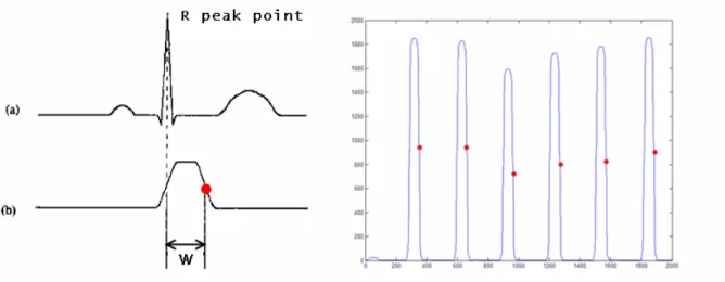
(35) The slope of the R wave alone is not a guaranteed way to detect a QRS event. Many abnormal QRS complexes that have large amplitudes and long durations (not very steep slopes) might not be detected using information about slope of the R wave only. Thus, we need to extract more information from the signal to detect a QRS event. Moving window integration extracts features in addition to the slope of the R wave. It is implemented with the following difference equation (3.4). For a sample rate of 500 sps, the integration window chosen for implementation in the thesis is 64 samples wide (which correspond to 128 ms). After the preprocessing stage, the peak detection stage detects peaks in the signals after moving window average. The corresponding relation between ECG raw data and the signals after moving window average is shown in Fig. 3.10. The detection algorithm stores the maximal levels encountered in the signal since the last peak detection like the red dots in Fig. 3.10. A new peak is defined only after a level is encountered that is less than half the height of the maximal level. Detection occurs halfway down the back side of the peak. This approach eliminates multiple detections from ripple around the wave peak. The peak detection algorithm does not establish that a valid peak has occurred until the middle of the falling slope when the level drops below half the distance from the maximal value to the base point. Because the time between the middle of the rising slope and the middle of the falling slope is equal to the duration of the averaging window, ideally the R peak point representing the peak of the R wave is located with fixed delay of one window’s width. Each time a peak is detected it is classified as either a QRS complex or noise, or it is saved for later classification. This work uses the peak height and peak location to classify peaks. An outline of the basic detection rules in the peak detection stage are listed as follows. 1. Ignore all peaks that precede or follow larger peaks by less than 200ms. 2. If the peak is larger than the detection threshold call it a QRS complex, otherwise call it noise.. Moving − Window Integral y (nT ) = (1 N ) ⎡⎣ x ( nT − ( N − 1)T ) + x ( nT − ( N − 2)T ) + ... + x ( nT ) ⎤⎦ where N is the number of samples in the width of the integration window. 23. (3.4).

(36) Fig. 3.10: The corresponding relation between ECG raw data and the signals after moving window average. 3.1.3 Evaluating the QRS detection algorithm Many algorithm of HRV analysis, such as heart rate calculation, PAV detection, and PVC detection, require a very accurate QRS recognition capability. Several standard ECG database are available for the evaluation of software QRS detection algorithms. Tests on these well-annotated and validated databases provide reproducible and comparable results. Furthermore, these databases contain many selected signals representative for the large variety observed but clinically important. The MIT-BIH Arrhythmia Database is the most frequently used database. It contains 48 half-hour recordings of annotated ECG with sampling rate of 360Hz and 11-bit resolution over a 10mV range. Twenty-five recordings with less common arrhythmias were selected from over 4000 24-hour ambulatory ECG recordings, and the rest was chosen randomly. While some records contain clear R-peaks and few artifacts (e.g., records 100-107), for some records the detection of QRS complexes is very difficult due to abnormal shapes, noise, and artifacts (e.g., records 108 and 207). The MIT-BIH Arrhythmia Database is acquired from the PhysioNet which offers free access via the web to large collections of recorded physiologic signals and related open-source software [26]. There are forty-eight recordings in this database. Each recording include annotations that indicate the times of occurrence and types of each individual heart 24.

(37) beat ("beat-by-beat annotations"). The standard set of annotation codes includes both beat annotations and non-beat annotations. Most PhysioBank databases use these codes as described as Table A.1 in Appendix A. According to [22], essentially three parameters should be used to evaluate the QRS detection algorithm. They are formulated as (3.5) where TP denotes the number of true positive detection, FN denotes the number of false negatives, and. FP denotes the number of false positives. Therefore, TP represents the QRS detector successfully detects the beats which are coded by beat annotations, FN represents the QRS detector misses the beats which are coded by beat annotations and FP means the QRS detector detects the beats which are coded by non-beat annotations or non-existed actually. In this study, all the forty-eight recordings in the MIT-BIH Arrhythmia Database are used to evaluate the QRS detector algorithm. Each recording records half-hour annotated ECG, but just first ten minutes data are used to evaluate the QRS detector performance for simplicity. The evaluation result of each recording is listed in Table A.2 of Appendix A and the performance measures are listed in Table 3.1.. 3.1.4 Abnormal Beats Rejection and Compensation The heart beat is triggered mainly by the sinoatrial (SA) node controlled by the sympathetic and parasympathetic neural systems. In addition to the SA node, other latent. Sensitivity =. TP TP + FN. TP TP + FP ∑ Detected QRS time − Actual QRS time Average Time error (ms ) = TP. Positive predictivity =. Table 3.1: The performance of simplified algorithm adopted in this work. Sensitivity. Positive Predictivity. Average Time Error(ms). 95.65%. 99.36%. 5.33. 25. (3.5).

(38) pacemakers exist throughout the heart. Normally, regular conduction of the electrical impulse from the SA node and the refractory period of the cells reject any other electrical source except those coming from the SA node. However, some of the additional pacemakers may, in certain cases, interpose additional electrical impulses that generate ectopic beats. Besides, QRS complex misdetections can generate a similar effect to that of ectopic beats in HRV analysis [27]. The detector errors can be false positive (FP) when a false beat is detected due to noise or a high amplitude T wave or false negative (FN) when a real beat is missed due to a low amplitude QRS or noise masking. The abnormal beats make the time associated with HRV exhibit a sharp peak and make the power spectral density estimation in the frequency domain analysis strongly unstable shown in Fig. 3.10(a). In this study, the criterion based on the variation of the instantaneous heart rate is used as the abnormal beats detector [27]. The normal heart beat shows a band limited variation of the instantaneous heart rate. So, it is possible to impose a threshold TH on the derivative of the instantaneous heart rate to screen out the abnormal beats. The criterion is formulated as (3.6). The threshold TH is set to 0.2 empirically in this study. When the criterion in (3.6) is not met for some peak time instant tk , it means that some position tk −1 , tk , or tk +1 are abnormal. The six conditions which judge whether the anomalies were caused by QRS complex misdetections or not is checked all over the recorded data: by removing tk , removing tk +1 , inserting an intermediate beat between tk −1 and tk , inserting an intermediate beat between tk and tk +1 , moving tk to the intermediate position between tk −1 and tk +1 , and moving tk +1 to the intermediate position between tk and tk + 2 . If the criterion is now satisfied when removing, it implies a FP at the removal position; if the criterion is satisfied on insertion, this implies a FN and if satisfied when moving it typically implies an ectopic beat. It can be found that almost all of the abnormal beats are produced by QRS complex. rˆk′ =. 1 1 − t −t t −t = k +1 k k k −1 ≤ TH tk +1 − tk −1. tk −1 − 2tk + tk +1 ( tk −1 − tk )( tk −1 − tk +1 )( tk − tk +1 ). (3.6). unit :. ms. ( ms ). 3. =. 1. ( ms ). 2. =. 1. ( s *10 ). −3 2. =. 1 ⋅106 2 s. 26.

(39) misdetection from the collected data in the experiment. There is a data filtering mechanism existing in this study for data accuracy and stability. There are two criteria for each HRV analysis section in one ECG recording. First, the number of detected abnormal beats in each HRV analysis section must be lower than 5. Second, it must be confirmed that there is not any abnormal beat remaining after the abnormal beat processing in each HRV analysis section. If any one criterion is not satisfied in any analysis section of one ECG recording, the ECG recording will be looked as the unstable data and be abandoned. A simple method for abnormal beats processing is utilized and the detailed algorithm is formulated in Appendix B. It can be seen in Fig. 3.10(b) that the more stable and accurate spectrum analysis can be obtained after the removing and compensating of these abnormal beats.. Fig. 3.11(a) Abnormal beats detection. Fig. 3.11(b) Abnormal beats removement and compensation. 27.

(40) Fig. 3.12: The RR interval time series after 4Hz cubic spline interpolation.. 3.1.5 Interpolation and De-trending. 3.1.5.1 Interpolation The RR interval time series is an irregularly time-sampled signal. This is not an issue in time domain analysis, but in the frequency domain analysis it has to be taken into account. If the spectrum estimate is calculated from this irregularly time-sampled signal, implicitly assuming it to be evenly sampled, additional harmonic components are generated in the spectrum. Therefore, the RR interval signal is usually interpolated before the spectral analysis to recover an evenly sampled signal from the irregularly sampled event series. The RR interval time series after interpolation is shown in Fig. 3.11. The 4Hz cubic spline interpolation is used in this study [28]. The fundamental idea behind cubic spline interpolation is based on the engineer’s tool used to draw smooth curves through a number of points as shown in Fig. 3.12. The mathematical spline is similar in principle. The points, in this case, are numerical data. The weights are the coefficients on the cubic polynomials used to interpolate the data. These 28.

(41) Fig. 3.13: The fundamental idea behind cubic spline interpolation. coefficients ’bend’ the line so that it passes through each of the data points without any erratic behavior or breaks in continuity. The essential idea is to fit a piecewise function of the form shown as (3.6). And si is a third degree polynomial function defined by (3.7) for. i = 1, 2,… , n − 1 . In this work, “natural splines” which include the stipulation that the second derivative be equal to zero at end point is adopted. By the four properties of cubic splines listed in (3.8), the weights can be determined by the matrix equation (3.9) and (3.10). The iterative method to solving M i is shown as (3.11) for the future hardware implementation.. ⎧ s1 ( x ) if ⎪ ⎪ s ( x ) if S ( x) = ⎨ 2 ⎪ ⎪ ⎩ sn −1 ( x ) if. x1 ≤ x < x2 x2 ≤ x < x3 xn −1 ≤ x < xn. si ( x ) = ai ( x − xi ) + bi ( x − xi ) + ci ( x − xi ) + di 3. 2. (1). The piecewise function S ( x ) will interpolate all data points.. (2). S ( x ) will be continuous on the interval [ x1 , xn ] .. (3). S ' ( x ) will be continuous on the interval [ x1 , xn ] .. (4). (3.6). S '' ( x ) will be continuous on the interval [ x1 , xn ] .. 29. (3.7). (3.8).

(42) ⎡4 ⎢ ⎢1 ⎢0 ⎢ ⎢ ⎢0 ⎢ ⎢0 ⎢0 ⎣. ai =. 1 0 4 1 1 4 0 0 0 0 0 0. ⎡ y1 − 2 y2 + y3 ⎤ ⎢ ⎥ ⎢ y2 − 2 y3 + y4 ⎥ ⎢ y3 − 2 y4 + y5 ⎥ ⎢ ⎥ ⎢ ⎥ ⎢ yn − 4 − 2 yn − 3 + yn − 2 ⎥ ⎢ ⎥ ⎢ yn −3 − 2 yn − 2 + yn −1 ⎥ ⎢ ⎥ ⎣ yn − 2 − 2 yn −1 + yn ⎦. 0 0 0⎤ ⎡ M 2 ⎤ 0 0 0 ⎥⎥ ⎢⎢ M 3 ⎥⎥ 0 0 0⎥ ⎢ M 4 ⎥ 6 ⎥ ⎥⎢ = 2 ⎢ ⎥ ⎥ xi − xi −1 ) ( ⎢ ⎥ ⎥ 4 1 0 M n −3 ⎥ ⎥⎢ 0 4 1 ⎥ ⎢ M n−2 ⎥ 0 1 4 ⎥⎦ ⎢⎣ M n −1 ⎥⎦. M i +1 − M i M bi = i 6 ( xi − xi −1 ) 2. ci =. yi +1 − yi ⎛ M i +1 + 2M i ⎞ −⎜ ⎟ ( xi − xi −1 ) di = yi h 6 ⎝ ⎠. (3.9). (3.10). for i = 0 : ( n − 1) hi = xi +1 − xi. bi = ( yi +1 − yi ) hi end u1 = 2 ( h0 + h1 ) v1 = 6 ( b1 − b0 ) for i = 2 : ( n − 1) ui = 2 ( hi −1 + hi ) −. hi2−1. vi = 6 ( bi − bi −1 ) −. hi −1vi −1. ui −1 ui −1. end Mn. for i = ( n − 1) : −1:1 Mi =. ( vi − hi zi +1 ) ui. end M0 = 0. 30. (3.11).

(43) Fig. 3.14: The RR interval time series after de-trending.. 3.1.5.2 Detrending Heart rate variability (HRV) is widely used quantitative marker of autonomic nervous system activity. Various time and frequency domain methods have been applied to HRV analysis. A traditional spectral method, power spectral density (PSD) estimation, provides information about power distribution as a function of frequency. Spectral estimation inherently assumes that the signal is at least weakly stationary. However, real HRV is usually non-stationary. Non-stationarities like slow linear or more complex trends in the HRV signal can cause distortion to time and frequency domain analysis. Origins for non-stationarities in HRV are discussed [15].. The method tries to remove the slow non-stationary trends from the. HRV signal before analysis is called de-trending. The detrending is usually based on first-order or higher order polynomial models. In this thesis, an advanced detrending procedure based on smoothness priors approach is adopted [29]. The main advantage of the method is its simplicity. The frequency response of the method is adjusted with a single parameter. This smoothing parameter should be selected in such a way that the spectral components of interest are not significantly affected by the detrending. The RR interval time series after de-trending is shown in Fig. 3.13. The detailed processing flow of detrending is explained as follows: The RR interval time series is denoted as (3.12). The detrended nearly stationary RR series can be calculated as (3.13) where the second-order difference matrix D2 ∈ 31. ( N −3)×( N −1).

(44) z = ( R2 − R1 , R3 − R2 ,..., RN − RN −1 ). T. (. 0 1 1. N −1. (3.12). )z. (3.13). 0⎞ ⎟ ⎟ 0⎟ ⎟ −2 1 ⎠. (3.14). zˆstat = I − ( I + λ 2 D2T D2 ) ⎛ 1 −2 1 ⎜ 0 1 −2 ⎜ D2 = ⎜ ⎜ 0 ⎝0. ∈. −1. is shown as (3.14). The frequency response of the detrending method is detailed as follows. Equation (3.13) can be written as zˆstat = Lz , where L = I − ( I + λ 2 D2T D2 ). −1. corresponds to a. time-varying finite-impulse response high-pass filter. The frequency response of L for each discrete time point, obtained as a Fourier transform of its rows, is presented in Fig. 3.14. The filtering effect is attenuated for the first and last elements of z and, thus, the distortion of end points of data is avoided. The effect of the smoothing parameter λ on the frequency response of the filter is presented in Fig. 3.15. The cutoff frequency of the filter decreases when λ is increased. Besides, the λ parameter the frequency response naturally depends on the sampling rate of signal z . Because each RR series is first interpolated to obtain a regularly sampled series with sampling rate of 4Hz, the smoothing parameter λ is set to 300, which equals a cutoff frequency of 0.043 Hz.. Fig. 3.15: Time-varying frequency response of L ( N − 1 = 50 and λ = 10 ) . Only the first half of the frequency response is presented, since the other half is identical 32.

(45) Fig. 3.16 Frequency responses, obtained from the middle row of L , for λ = 1, 2, 4, 10, 20, 50, and 300. The corresponding cutoff frequencies are 0.189, 0.132, 0.093, 0.059, 0.041, 0.025, and 0.011 times the sampling frequency. 3.1.6 Measures of Heart Rate Variability There are many measures and analyzing methods of heart rate variability have been proposed such as time domain analysis, frequency domain analysis, linguistic analysis, etc. Although many other measures of HRV have been proposed and investigated, those specified by the Task Force of the European Society of Cardiology and the North American Society of Pacing and Electrophysiology (the Task Force) have been the most widely applied [3]. In this study, time and frequency domain analysis are the main methods used to observe the changes of physiological responses. The effect of synchronization can be observed by the time domain analysis and the modulation of autonomic nervous system can be observed by the frequency domain analysis.. 3.1.6.1 Time domain measures The Task Force specified many different HRV metrics for both short-term records (5min) and long-term records (24h). Taking the reliability and accuracy of heart rate variability 33.

(46) measurements into account [30], I choose THB (total heart beats), MRR (mean of RR intervals), SDNN (standard deviation of normal to normal) and RMSSD (root mean square of successive NN interval differences) as the time domain measurements in this study. The detailed calculation formulas are shown by the following equation (3.12). Here, N is the total number of the heart beats and I ( n ) is a time series of beat-to-beat intervals which can be referred to Fig. 2.9. 3.1.6.2 Frequency domain measures While the time domain measures help in assessing the magnitude of the temporal variations in the autonomically modulated cardiac rhythm, the frequency domain analysis provides the spectral composition of these variations. All frequency domain HRV metrics are based on the estimated power spectral density (PSD) of the NN (Normal to Normal) intervals. Although the Task Force gave specific definitions of these metrics, it did not specify how to estimate the PSD. There are many methods of estimating PSD and each generates different HRV metric values. In this section we give a complete description of our PSD estimator, as required by the Task Force. Power spectral density (PSD) analysis provides the basic information of how power (i.e. variance) distributes as a function of frequency. Methods for the calculation of PSD may be generally classified as non-parametric and parametric [31]. Due to the simplicity of the algorithm (Fast-Fourier Transform) and high processing speed, non-parametric method, Welch method, is chosen to estimate the power spectral density [32]. The detailed procedure of power spectral analysis in this study is explained as. THB = N MRR =. 1 N ∑I (n) N −1 n=2. (. 1 N SDNN = ∑ I (n) − I N − 2 n=2 RMSSD =. ). 2. I=. 1 N ∑I (n) N −1 n=2. 1 N 2 [ I (n) − I (n −1)] ∑ N − 2 n=3 34. (3.12).

(47) follows: 1. The signal is split up into overlapping segments: The original data segment is split up into K data segments of length L (zero padding), overlapping by L/2 points (L=1024 in this study). 2. The overlapping segments are then windowed by the Hamming window. 3. After doing the above, the periodogram is calculated by computing the discrete Fourier transform, and then computing the squared magnitude of the result. The individual periodograms are then time-averaged, which reduces the variance of the individual power measurements. The end result is an array of power measurements vs. frequency bin. Through the use of computationally efficient algorithms such as Fast-Fourier Transform, the HRV signal is decomposed into its individual spectral components and their intensities, using Power Spectral Density (PSD) analysis. These spectral components are then grouped into three distinct bands: very-low frequency (VLF), low frequency (LF) and high frequency (HF). The cumulative spectral power in the LF and HF bands and the ratio of these spectral powers (LF/HF) has demonstrable physiological relevance in healthy and disease states [33, 34]. Changes in the LF band spectral power (0.04-0.15Hz frequency range) reflect a. Table 3.2: The HRV measures of time and frequency domain analysis Variable. Units. Description Time domain analysis. THB MRR. ms. Total number of heart beats Mean of RR interval. SDNN. ms. Standard deviation of all RR intervals.. ms. The square root of the mean of the sum of the squares of differences between adjacent NN intervals.. RMSSD. Frequency domain analysis. LF. ms 2. Power in low frequency range 0·04–0·15 Hz. HF. ms 2. Power in high frequency range 0·15–0·4 Hz. LF/HF. /. Ratio LF /HF 35.

(48) combination of sympathetic and parasympathetic ANS outflow variations, while changes in the HF band spectral power (0.15-0.40Hz range) reflect vagal modulation of cardiac activity. The physiological explanation of the VLF component (0.0033-0.04Hz) is much less defined and the existence of a specific physiological process attributable to these heart period changes might even be questioned. The LF/HF power ratio is used as an index for assessing sympatho-vagal balance. The HRV measures of time and frequency domain analysis we want to observe are listed in Table 3.2.. 3.2. Drum loop rhythmic analysis Sound by its very nature is temporal, and in its most generic sense, the word rhythm is. used to refer to all of the temporal aspects of a musical work, whether represented in a score, measured form a performance, or existing only in the perception of the listener [35]. The drum loop music is taken as the stimuli in this study because of its obvious and simple rhythm characteristic. Drum loops are prerecorded percussive riffs that are designed to create a continuous beat or pattern when played repeatedly. Loops are usually compiled in commercially available databases containing several hundreds, or even thousands, of these riffs. These collections are widely used in computer music composition and production as a means to generate high-quality music tracks in a quick and easy manner. This study utilizes the techniques in the field of audio signal processing and music analysis to extract some features from the drum loops and discusses their effects on the modulation of autonomic nervous system. Entrainment describes a process whereby two rhythmic processes interact with each other in such a way that they adjust towards and eventually ‘lock in’ to a common phase and/or periodicity [7]. For example, we tap foot and shake body to the beat of a song. Similarly, there are many naturally occurring rhythms within the human body such as the heartbeat, blood circulation, respiration and many others. Therefore, the relationship between the musical rhythmic characteristics and heart rhythm is what this study wants to explore. So the next problem is how to quantitatively define the musical characteristic, rhythm. Intuitively, the first feature of rhythm is its speed. The speed of heart rhythm is called heart rate and the speed of musical rhythm is called tempo. Tempo is usually indicated in beats per 36.

(49) Fig. 3.17(b): Onset, attack and transient. Fig. 3.17(a): The sound wave of one single note. minute (BPM) in modern music. The beat means the exact time we nod our head or tap our feet to the rhythm. It is one temporal aspects of a musical work existing in the perception of the listener and a fundamental unit of the temporal structure of music. Once the beats in one piece of music were detected, the tempo could be decided as the unit, beats per minute. Is the tempo enough to describe the musical rhythm fully? Through the automatic beat tracking algorithm, each onset in a piece of music which probably makes us tap to follow will be identified. And it can be found that the intervals between each identified beat are almost the same. If the other components of a piece of music were removed except the beats, the remains are only the repeated and equal spaced sound pulses. These pulses can’t make us feel rhythmic. So it is not enough to represent the musical rhythm by the only one feature, tempo. Observing the characteristics of heart rhythm, it can be found the variability of heart rate exists in a stable and near constant heart rate. Inspired by the similarity, the second feature, complexity, is proposed to be the second quantitative measure to describe the musical rhythm. As the tempo is to musical rhythm, so is the average heart rate to the heart rhythm. As the complexity is to musical rhythm, so is the heart rate variability to the heart rhythm. That’s why the feature, complexity, is chosen. The heart rhythm is just like a piece of music. If it is just a monotone pulse, it will be not good to listen, in other words, not a healthy heart rhythm.. 3.2.1 Tempo To find the exact time when we nod our heads or tap our feet is called “beat tracking.” 37.

(50) Automatic beat tracking is an essential task for many applications such as musical analysis, automatic rhythm alignment of multiple musical instruments, cut and paste operations in audio editing, beat driven special effects. Music is expressed by the successive notes. These notes record the relating temporal information. Identifying and characterizing these notes is an important aspect of the following steps of music analysis. Here some nouns must be explained first. In the Fig. 3.14 (a), the sound wave of one single note is shown. The definitions of onset, attack and transient are shown in Fig. 3.14(b) and were explained in [36]. An onset can be defined as the instant when the attack transient begins, thus marking the beginning of the note. So the first step of music analysis is to detect the onset. In the general case of a polyphonic signal, where multiple sound objects may be present at a given time, the onset detection is not easy. The procedure employed in the majority of onset detection algorithms is illustrated in Fig. 3.15: from the original audio signal, which can be pre-processed to improve the performance of subsequent stages, a detection function is derived at a lower sampling rate, to which a peak-picking algorithm is applied to locate the onsets. Once the rhythmic events (the onsets) have been determined, the beat tracking algorithm will be applied. The beat tracking algorithm adopted in this work is developed by Simon Dixon [37]. First, the time intervals between pairs of events are determined. These data are. Fig. 3.18: Flowchart of a standard onset detection algorithm 38.