適用於H.264視訊晶片之功率感知編碼系統

(1)

國立交通大學

電子工程學系電子研究所碩士班

碩士論文

適用於 H.264 視訊晶片之功率感知編碼系統

Power-Aware Coding for H.264 Video Chip

研究生: 張瑋城

指導教授: 張添烜

(2)

(3)

適用於 H.264 視訊晶片之功率感知編碼系統

Power-Aware Coding for H.264 Video Chip

研究生: 張瑋城 Student: Wei-Cheng Chang

指導教授: 張添烜博士 Advisor: Tian-Sheuan Chang

國立交通大學電子工程學系電子研究所碩士班

碩士論文

A Thesis

Submitted to Department of Electronics Engineering & Institute of Electronics College of Electrical Engineering and Computer Science

National Chiao Tung University in Partial Fulfillment of Requirements

for the Degree of Master of Science

In

Electrical Engineering November 2008

Hsinchu, Taiwan, Republic of China

(4)

(5)

i

適用於 H.264 視訊晶片之功率感知編碼系統

研究生：張瑋城指導教授：張添烜博士國立交通大學電子工程學系電子研究所

摘要

有限的電池容量，一直都是多媒體手持裝置使用時間上的主要考量，所以具有功率感知功能的視訊編碼系統逐漸在相關裝置上盛行，然而，之前相關研究中，以軟體為基礎的方法雖然可以達到功率-碼率-失真的最佳化，但是其中從處理器觀點所發展出的公式及模型不適用於用途特殊積體電路設計上，另一方面，以硬體為基礎的方法雖然可以根據不同的操作環境來調整功率消耗，可是整體碼率與失真的效能並沒有被考慮到。為了解決以上的問題，本篇研究提出了一個功率感知編碼系統適用於 H.264 視訊晶片，在滿足功率限制的情況下，我們提出的方法使用碼率-失真代價來預測且分配功率給每一個宏塊，根據內容來決定此宏塊相對應之編碼情形來達到碼率與失真的效能最佳化，如此一來，功率可以有效的被使用在編碼。實驗模擬的結果顯示出，在較靜態的視訊且百分之 65 的功率限制下，我們提出的方法可以達到和全功率近乎相同的碼率與失真，且同時只會消耗百分之 32.5 的功率；對於較動態的視訊而言，我們提出的方法可以將功率限制所造成較差的碼率與失真減到最低，而且在同樣功率限制下，相較於沒有功率感知的方法，峰值信噪比可提升多於 1dB。

(6)

(7)

iii

Power-Aware Coding for H.264 Video Chip

Student: Wei-Cheng Chang Advisor: Dr. Tian-Sheuan Chang

Department of Electronics Engineering & Institute of Electronics National Chiao Tung University

Abstract

Limited battery capacity is always a major concern for increasing the working time of mobile multimedia devices. Thus, power-aware video coding has become popular in recent researches. However, previous works on software-based approaches are optimized on power-rate-distortion, but not suitable for ASIC design due to its processor-based formulation and modeling. On the other hand, hardware-based approaches only directly adjust its power consumption in response to different operating conditions without considering rate-distortion (RD) performance.

Being aware above problems, this thesis proposed a power-aware video coding suitable for dedicated H.264 ASIC design. The proposed method uses encoded rate-distortion (RD) cost to predict and allocate the power for each macroblock (MB) under the given power constraint. Then the corresponding intra modes and inter modes are selected based on content to maximize the RD performance. Thus, simple MBs will have less power allocation while complex MBs will have more power for better overall RD performance.

The simulation result shows that the proposed method at 65% of power constraint can achieve nearly the same quality and bit rate as that in full power mode but only consumes 32.5% of full power for low motion sequences. For high motion sequences, the proposed method can degrade the quality gracefully for increasingly lower power supply, and achieves more than 1dB higher at PSNR compared with non power-aware scheme.

(8)

(9)

v

誌謝

首先，要感謝我的指導教授—張添烜博士，這兩年來給我的支持和鼓勵，引領我以正確的態度來面對與解決問題。在研究上，總是讓我能自由的發揮，並在遇到瓶頸的時候給予建議與協助。此外感謝老師提供豐富的實驗室資源，使我不但能充分的利用軟硬體設備來進行研究，老師不僅是研究上的良師也是生活上的益友，不僅了解學生的想法也協助學生處理生活上的各種問題。謝謝我的口試委員們，清大電機陳永昌教授和交大資工彭文孝教授，感謝你們百忙中抽空來指導我，因為你們寶貴的意見讓我的論文更加完備。感謝 VSP 實驗室的好伙伴們，特別要謝謝引我入門的林佑昆學長，帶領我從零開始，一點一滴的從研究中學習與成長，尤其是當我對困難感到迷惘時，總是不厭其煩的和我討論，並且提供我許多寶貴的意見與想法。感謝張彥中學長、李國龍學長，你們對於經驗與知識的分享，讓我受用無窮。謝謝李得瑋學長、郭子筠學長和廖英澤學長耐心的教導我許多硬體設計的觀念與技巧，也感謝林嘉俊學長與吳秈璟學長，你們在研究上認真負責的態度是我學習的榜樣。感謝戴瑋呈、蔡宗憲和詹景竹同學不時的給予研究上的幫忙與協助，能跟你們一起討論是一段很難得的過程。感謝黃筱珊學妹、陳之悠、沈孟維、許博淵、蔡政君與廖元歆學弟們，有你們的陪伴，我的碩士班生涯充滿了歡笑。謝謝實驗室的所有成員們，和你們一起努力的日子，都是我在交大寶貴的回憶。最後要感謝默默支持我的家人們，我的爸媽與姊姊，你們的溫暖是我努力最大的支柱。在此，把本論文獻給所有愛我與所有我愛的人。

(10)

(11)

vii

1. INTRODUCTION ... 2 1.1. BACKGROUND ... 2 1.2. RELATED WORK ... 2 1.3. MOTIVATION AND CONTRIBUTION ... 3 1.4. ORGANIZATION OF THE THESIS ... 4 2. OVERVIEW OF H.264 STANDARD AND ENCODER CHIP ... 5 2.1. OVERVIEW OF H.264 STANDARD ... 5 2.1.1. Encoding Structure ... 5 2.1.2. Variable Block Size Motion Estimation ... 6 2.1.3. Quarter‐Pixel Resolution Motion Vector ... 6 2.1.4. Directional Intra Prediction ... 6 2.1.5. In‐Loop Deblocking Filter ... 7 2.1.6. Context Adaptive Entropy Coding ... 7

2.2. OVERVIEW OF H.264 ENCODER CHIP ... 8

2.2.1. Overview of H.264 Encoder Chip ... 8

2.2.2. Power Consumption of H.264 Encoder Chip ... 9

3. REVIEW OF POWER‐AWARE VIDEO ENCODER ... 11

3.1. REVIEW OF SOFTWARE‐BASED POWER‐AWARE VIDEO ENCODER ... 12

3.2. REVIEW OF HARDWARE‐BASED POWER‐AWARE VIDEO ENCODER ... 14

4. PROPOSED HARDWARE ORIENTED POWER‐AWARE ALGORITHM ... 16

4.1. CONCEPT OF POWER CONSTRAINT AND POWER BUDGET ... 17

(12)

viii

4.3. SKIP MODE DETECTION AND IME POWER ALLOCATION ... 21

4.4. PROPOSED FME POWER ALLOCATION ... 22

4.5. PROPOSED INTRA POWER ALLOCATION ... 25

4.5.1. SADThd_INTRA4x4 ... 26

5. SIMULATION AND ANALYSIS ... 28

5.1. POWER CONSTRAINT PATTERN ... 29

5.2. SIMULATION RESULT ... 30 5.2.1. Rate‐Distortion Performance ... 31 5.2.2. Power‐Distortion Performance ... 36 5.2.3. Power Comparison ... 41 5.2.4. Distribution of Skip Mode ... 44 5.2.5. Distribution of INTRA MB ... 49 6. CONCLUSION AND FUTURE WORK ... 52 6.1. CONCLUSION ... 52 6.2. FUTURE WORK ... 52 7. REFERENCE ... 53

(13)

ix

LIST OF FIGURES

FIGURE 2‐1 THE BASIC STRUCTURE OF ENCODER [13] ... 6

FIGURE 2‐2 SYSTEM OVERVIEW OF H.264 HIGH PROFILE ENCODER [14] ... 9

FIGURE 2‐3 POWER PROFILE OF H.264 VIDEO ENCODER ... 10

FIGURE 3‐1 P‐R‐D MODEL [7] ... 13

FIGURE 3‐2 RATE‐DISTORTION CURVE OF [10], FOREMAN CIF ... 15

FIGURE 3‐3 POWER‐DISTORTION CURVE OF [10], FOREMAN CIF @ 700 KBPS ... 15

FIGURE 4‐1 POWER BUDGET CONCEPT ... 18

FIGURE 4‐2 FLOW CHART OF PROPOSED POWER‐AWARE ALGORITHM ... 20

FIGURE 4‐3 FLOW OF SKIP MODE DECISION AND IME POWER ALLOCATION ... 21

FIGURE 4‐4 FLOW OF FME POWER ALLOCATION ... 22

FIGURE 4‐5 POWER CONSUMPTION OF 1‐MODE AND 2‐MODE FME ... 23

FIGURE 4‐6 FLOW OF INTRA POWER ALLOCATION ... 26

FIGURE 5‐1 EXAMPLE OF POWER CONSTRAINT OF 80 ... 29

FIGURE 5‐2 RD CURVES OF PA W/O SKIP UNDER DIFFERENT POWER CONSTRAINTS FOR “AKIYO” ... 32

FIGURE 5‐3 RD CURVES OF PA W/ SKIP UNDER DIFFERENT POWER CONSTRAINTS FOR “AKIYO” ... 32

FIGURE 5‐4 RD CURVES OF PA W/O SKIP UNDER DIFFERENT POWER CONSTRAINTS FOR “FOREMAN” ... 33

FIGURE 5‐5 RD CURVES OF PA W/ SKIP UNDER DIFFERENT POWER CONSTRAINTS FOR “FOREMAN” ... 33

FIGURE 5‐6 RD CURVES OF PA W/O SKIP UNDER DIFFERENT POWER CONSTRAINTS FOR “FOOTBALL” ... 34

FIGURE 5‐7 RD CURVES OF PA W/ SKIP UNDER DIFFERENT POWER CONSTRAINTS FOR “FOOTBALL” ... 34

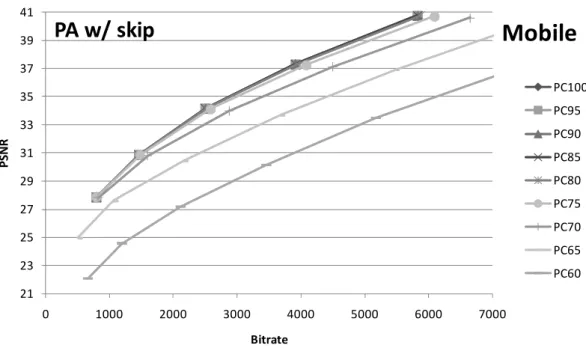
FIGURE 5‐8 RD CURVES OF PA W/ SKIP UNDER DIFFERENT POWER CONSTRAINTS FOR “MOBILE” ... 35

FIGURE 5‐9 RD CURVES OF PA W/ SKIP UNDER DIFFERENT POWER CONSTRAINTS FOR “MOBILE” ... 35

FIGURE 5‐10 POWER‐DISTORTION CURVE ... 36

FIGURE 5‐11 P‐D CURVES OF PA W/O SKIP AND PA W/ SKIP FOR “AKIYO” AT LOW BITRATE 150(KB/S) ... 37

(14)

x

FIGURE 5‐13 P‐D CURVES OF PA W/O SKIP AND PA W/ SKIP FOR “AKIYO” AT HIGH BITRATE 550(KB/S) ... 37

FIGURE 5‐14 P‐D CURVES OF PA W/O SKIP AND PA W/ SKIP FOR “FOREMAN” AT LOW BITRATE 400(KB/S) ... 38

FIGURE 5‐15 P‐D CURVES OF PA W/O SKIP AND PA W/ SKIP FOR “FOREMAN” AT MEDIAN BITRATE 1300(KB/S) ... 38

FIGURE 5‐16 P‐D CURVES OF PA W/O SKIP AND PA W/ SKIP FOR “FOREMAN” AT HIGH BITRATE 2200(KB/S) ... 38

FIGURE 5‐17 P‐D CURVES OF PA W/O SKIP AND PA W/ SKIP FOR “FOOTBALL” AT LOW BITRATE 1000(KB/S) ... 39

FIGURE 5‐18 P‐D CURVES OF PA W/O SKIP AND PA W/ SKIP FOR “FOOTBALL” AT MEDIAN BITRATE 2300(KB/S) ... 39

FIGURE 5‐19 P‐D CURVES OF PA W/O SKIP AND PA W/ SKIP FOR “FOOTBALL” AT HIGH BITRATE 3600(KB/S) ... 39

FIGURE 5‐20 P‐D CURVES OF PA W/O SKIP AND PA W/ SKIP FOR “MOBILE” AT LOW BITRATE 1200(KB/S) ... 40

FIGURE 5‐21 P‐D CURVES OF PA W/O SKIP AND PA W/ SKIP FOR “MOBILE” AT MEDIAN BITRATE 3300(KB/S) ... 40

FIGURE 5‐22 P‐D CURVES OF PA W/O SKIP AND PA W/ SKIP FOR “MOBILE” AT HIGH BITRATE 5400(KB/S) ... 40

FIGURE 5‐23 POWER COMPARISON OF PA W/O SKIP AND PA W/ SKIP FOR “AKIYO” ... 42

FIGURE 5‐24 POWER COMPARISON OF PA W/O SKIP AND PA W/ SKIP FOR “FOREMAN” ... 42

FIGURE 5‐25 POWER COMPARISON OF PA W/O SKIP AND PA W/ SKIP FOR “FOOTBALL” ... 43

FIGURE 5‐26 POWER COMPARISON OF PA W/O SKIP AND PA W/ SKIP FOR “MOBILE” ... 43

FIGURE 5‐27 SKIP MODE DISTRIBUTION UNDER POWER CONSTRAINT FROM 95 TO 65 FOR “AKIYO” ... 45

FIGURE 5‐28 SKIP MODE DISTRIBUTION UNDER POWER CONSTRAINT 60 FOR “AKIYO” ... 45

FIGURE 5‐29 SKIP MODE DISTRIBUTION UNDER POWER CONSTRAINT FROM 95 TO 65 FOR “FOREMAN” ... 46

FIGURE 5‐30 SKIP MODE DISTRIBUTION UNDER POWER CONSTRAINT 60 FOR “FOREMAN” ... 46

FIGURE 5‐31 SKIP MODE DISTRIBUTION UNDER POWER CONSTRAINT FROM 95 TO 65 FOR “FOOTBALL” ... 47

FIGURE 5‐32 SKIP MODE DISTRIBUTION UNDER POWER CONSTRAINT 60 FOR “FOOTBALL” ... 47

FIGURE 5‐33 SKIP MODE DISTRIBUTION UNDER POWER CONSTRAINT FROM 95 TO 65 FOR “MOBILE” ... 48

FIGURE 5‐34 SKIP MODE DISTRIBUTION UNDER POWER CONSTRAINT 60 FOR “MOBILE” ... 48

(15)

xi

LIST OF TABLES

TABLE 4‐1 THE SADTHD_INTRA4X4 UNDER DIFFERENT POWERLEFTAVG ... 27

TABLE 5‐1 DISTRIBUTION OF INTRA MB FOR PA W/O SKIP AND PA W/ SKIP UNDER DIFFERENT POWER CONSTRAINTS FOR

“AKIYO” IN QP28 ... 50

“FOREMAN” IN QP28 ... 50

“FOOTBALL” IN QP28 ... 50

(16)

1

(17)

2

1. Introduction

1.1. Background

Mobile multimedia devices become very popular in our daily life with the fast development of semiconductor and communication technologies. In these devices, more novel and fancy multimedia functions are integrated in order to meet consumer’s endless demand for entertainments.

Thus the demand can be fulfilled by recent H.264 video coding standard [1] due to its outstanding coding efficiency and visual quality. The coding efficiency and visual quality are enhanced by powerful coding tools [2], such as variable block size motion estimation, directional intra prediction, context-based adaptive variable length coding, and in-loop de-blocking filter. At the same time, these powerful coding tools also lead to high power consumption overhead.

To support high power consumption of H.264 video coding on a mobile device with limited battery capacity, the emerging concept of power-aware design [3] [4] [5] [6] is expected to be introduced for further power optimization. The design idea is to provide more operating point between binary on and off state. As a consequence, the power-aware design helps extend the battery lifetime of mobile devices significantly.

1.2. Related Work

According to related works on power-ware video encoder, we separate them into two categories. One is the software-based approaches [7] [8] and the other is the hardware-based approaches [9] [10] [11] [12].

First, the software-based approaches are optimized on power-rate-distortion but not suitable for dedicated hardware due to its processor-based formulation and modeling.

(18)

3

Then, the hardware-based approaches have multiple power modes of operation and adapt the power mode according to the awareness of power constraints. However, the adaptation is only a look-up-table, and no further rate-distortion optimization is considered.

1.3. Motivation and Contribution

The issues mentioned above motivate us to develop a power-aware video coding system suitable for the H.264 ASIC design to maximize the rate-distortion performance while can dynamically meet different power constraints.

First, we analyze the encoding mechanism of our H.264 ASIC design and its power consumption of the major encoding modules. Then, we develop a corresponding video encoding architecture which adaptively controls the power consumption of power-demanding part by the proposed algorithm. The proposed algorithm dynamically allocates available power to each MB according to encoded RD cost in order to maximize the RD performance. Under such scheme, we further develop the following methods for these power-demanding parts.

1. We adopt a method of pre-skip mode detection to find if that is a pre-skip MB in order to save the most power consumption.

2. We propose fractional motion estimation (FME) power allocation method to determine appropriate power for FME encoding for maximizing RD performance.

3. We propose an INTRA power allocation method which can allocate essential power to INTRA-prone MB according to a content-adaptive threshold.

(19)

4

1.4. Organization of the Thesis

In this thesis, the H.264 video coding standard and our previous work on H.264 encoder chip will be introduced in Chapter 2. We review some recent works on power-aware encoder design in Chapter 3. The proposed hardware-oriented power-aware algorithm is presented in Chapter 4. We present the simulation result of our proposed algorithm in Chapter 5. Finally, conclusion and future work are in Chapter 6.

(20)

5

2. Overview of H.264 Standard and Encoder Chip

2.1. Overview of H.264 Standard

The H.264/AVC video coding standard [1] consists of a number of coding tools. Compared to the prior video coding standards, many important and new techniques can be found in [2]. Here, we would like to give a brief introduction of these tools, which have existed for some time but well integrated to form outstanding compression efficiency in H.264.

2.1.1. Encoding Structure

A simplified encoding flow of H.264 is shown in Figure 2-1 [13]. A video frame is first partitioned into a number of 16x16 Macro Blocks (MBs). Then each MB may go through the intra-prediction or the inter-prediction called motion unit called Motion Estimation (ME). The intra-prediction unit uses the neighboring block data to predict the current block. The inter-prediction unit uses the references frames to predict the current frame. Each predictor has a number of modes. A good design should pick up the best mode with the lowest rate and distortion. The prediction residuals are the transformed, quantized and entropy coding into the output encoded bitstream. In order to continue operating on the next incoming frame, the quantized current frame is reconstructed and stored.

(21)

6

Figure 2-1 the basic structure of encoder [13]

2.1.2. Variable Block Size Motion Estimation

In H.264, the standard defines the various block sizes for motion estimation. Seven kinds of block sizes are introduced, including 16x16, 16x8, 8x16, 8x8, 8x4, 4x8 and 4x4. It helps to enhance the efficiency of coding irregularly shaped objects or background behind moving objects.

2.1.3. Quarter-Pixel Resolution Motion Vector

The H.264 supports quarter-pixel resolution motion compensation, which is first found in the advanced profile of MPEG-4 Visual (Part 2) standard. It uses a 6-tap filter for interpolation.

2.1.4. Directional Intra Prediction

The H.264 uses the intra prediction techniques to reduce the spatial correlation inside a block. This technique estimates the current block prediction based on the previously encoded and reconstructed blocks. The intra prediction also adopts various-directional prediction modes to further enhance the coding efficiency.

(22)

7

2.1.5. In-Loop Deblocking Filter

In H.264, a filter is applied to every decoded macroblock in order to reduce blocking distortion caused by block-based transformation. In the encoder, the deblocking filter is applied after the inverse transform and before reconstructing and storing the macroblock for future predictions. In the decoder, it is applied before reconstructing and displaying the macroblock. The filter has two benefits: in the first place, block edges are smoothed, improving the appearance of decoded images, especially at higher compression ratios. In the second place, the filtered macroblock is used for motion-compensated prediction of further frames in the encoder, resulting in a smaller residual after prediction.

2.1.6. Context Adaptive Entropy Coding

Two entropy coding methods, Context-based Adaptive Binary Arithmetic Coding (CABAC) and Context-based Adaptive Variable Length Coding (CAVLC), are provided in H.264. Both methods contribute overall compression performance a lot.

(23)

8

2.2. Overview of H.264 Encoder Chip

2.2.1. Overview of H.264 Encoder Chip

In this section, we briefly overview our previous work on H.264 encoder chip [14]. We present the system overview in Figure 2-2. It focuses on high definition and high resolution video, and supports high profile coding tools. The new high profile coding tools are included as the shaded parts. The system architecture of the encoder has three MB-pipelining stages.

The first stage is the integer motion (IME) stage which occupies the most computation and memory resource of the entire H.264 encoder. For IME, we use a parallelized subsampling algorithm, Parallel Multi-Resolution ME (PMRME) [15]. It searches three subsampling levels of different search ranges in parallel so that all searches are done within 256 cycles in single step. After IME, we use Mode Filtering (MF) to select only two best modes for FME refinement so that FME tests at most 18 motion vectors instead of 41 motion vectors.

In the second stage, intra prediction and fractional motion estimation (FME) are placed in the same stage to share the current block buffer and pipelined buffer. As for FME, it searches only six candidates in a single step to improve the throughput. On the other hand, the intra prediction supports intra8x8, intra4x4 and intra16x16. It uses eight-pixel parallelism to solve the high throughput request and structure hazard.

The third stage is the entropy coding stage including Context-Adaptive Variable Length Coding (CAVLC) and Context-Adaptive Binary Arithmetic Coding (CABAC), which both provide high compression efficiency to generate the final bit-stream.

(24)

9

Figure 2-2 system overview of H.264 high profile encoder [14]

2.2.2. Power Consumption of H.264 Encoder Chip

The previous work focuses on high profile and high definition. However, the power consumption of previous work is too large to afford on mobile multimedia devices with small size resolution. As a consequence, we discard some power-hungry components, such as high profile coding tools, level-1 IME and level-2 IME, and form a modified design for our proposed power-aware H.264 encoder.

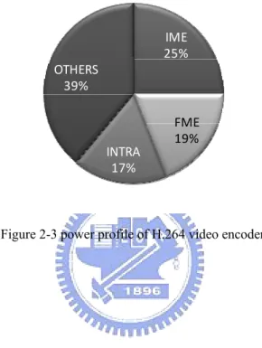
We generate power consumption result from PrimePower post-layout simulation. Our design is fabricated by UMC 0.13μm process. The required operating frequency is 7.2 MHz for Common Intermediate Format (CIF) sequence. The average power profile from different sequences is shown in Figure 2-3. The power consumption of IME only consists of PMRME level-0 mention before. The power consumption of FME is the 2-mode FME power consumption. The power consumption of INTRA consists of intra4x4 and intra16x16. The power consumption of OTHERS consists of

(25)

10

a number of necessary parts, such as external bus controller, global controller, current buffer, deblocking filter, and pipeline registers. Note that the power profile is 15% when the pre-skip mode detection [16] is occurred. We use the power profile generated here as a power database for developing the power-aware H.264 video encoder in Chapter 4.

Figure 2-3 power profile of H.264 video encoder

IME 25% FME 19% INTRA 17% OTHERS 39%

(26)

11

3. Review of Power‐Aware Video Encoder

The power-aware design concept [3] [4] [5] [6] has been introduced recently for further power optimization due to supporting high power consumption multimedia function, such as H.264 video coding, on a mobile device with limited battery capacity.

Simply speaking, a power-aware design is a smart design that is aware of the limiting power, and it can utilize the available power in a smart and efficient way by dynamically adjust its power consumption. The design idea is to provide more operating point between binary on and off state. For example, in a power-rich environment, a high quality service is preferred in spite of higher power consumption cost. On the other hand, if the battery capacity is low, users may allow poor quality service with lower power consumption. As a result, the power-aware design helps extend the battery lifetime of mobile devices significantly.

In this chapter, we partition the recent works on power-aware video encoder into two categories, software-based power-aware video encoder [7] [8] and hardware-based power-aware video encoder [9] [10] [11] [12].

(27)

12

3.1. Review of Software‐Based Power‐Aware Video Encoder

The rate-distortion analysis has been one of the major research focuses in information theory and communication for the past several decades, but there has been no analytic framework for modeling the power-rate-distortion (P-R-D) behavior of the video encoding system. Thus, the software-based power-ware video encoder designs are proposed to solve above issues.

First, they develop a MPEG-4 [18] video encoder architecture which is fully scalable in power consumption according to several control parameters. In other words, they introduce several control parameters into the video encoder to control the power consumption of major encoding modules by a complexity profiling of software-based encoder on CPU and a dynamic voltage scaling (DVS). Then, they analyze the rate-distortion behavior of these control parameters, and derive a comprehensive P-R-D model for the video encoding system. Finally, based on the P-R-D model, they develop a quality optimization scheme to determine the best configuration of complexity control parameter according to the power supply level of the mobile device to maximize the video presentation quality. Figure 3-1 show the proposed P-R-D model.

However, when we deal with the power-aware approach on ASIC design, the software-based approach is not suitable for dedicated hardware due to the processor-based formulation and modeling.

(28)

13

Figure 3-1 P-R-D model [7]

(29)

14

3.2. Review of Hardware‐Based Power‐Aware Video Encoder

In [6], this article provides an overview of power-aware video codec design concepts and approaches. From an ASIC design’s perspective, the focus will be more on how a dedicated architecture is able to being power-aware. A hardware-dedicated but parameter-reconfigurable architecture is a promising approach as it can meet the hard real-time processing requirement and also enable the power awareness. In this article, design perspectives and examples on power-aware motion estimation and discrete cosine transform will be discussed.

In [9] [10] [11] [12], they provide dedicated hardware designs with power-ware pre-skip detection, FME module, IME module and whole encoder respectively. From Figure 3-2 and Figure 3-3, we find that the hardware-based approaches have multiple power modes of operation, and can adapt its power mode according to the awareness of power constraints. In Figure 3-2 and Figure 3-3, the points from “a” to “b” represent high power consumption mode to low power consumption mode. For example, the point “a” represents 2 reference frames and 3-mode for FME processing. However, the adaptation is only a look-up-table, and no further rate-distortion optimization is considered.

(30)

15

Figure 3-2 rate-distortion curve of [10], foreman CIF

Figure 3-3 power-distortion curve of [10], foreman CIF @ 700 kbps

(31)

16

4. Proposed Hardware Oriented Power‐Aware

Algorithm

In this chapter, we present the proposed algorithm which is based on our previous work of H.264 high profile encoder reviewed in chapter 2. From chapter 3, we know that the related power-aware works on software-based approach and hardware-based approach still have room for improvement. The software-based approaches are not good solution to ASIC design. The hardware-based approaches are just a look-up-table way to adjust its power mode without further considering optimization on RD performance.

In order to achieve a power-aware functionality on ASIC design while can maximize the RD performance, the proposed algorithm dynamically allocates available power to each MB according to encoded RD cost. Then the corresponding intra and inter modes are selected based on content. Thus, simple MBs will have less power allocation while complex MBs have more power allocation for better overall RD performance.

(32)

17

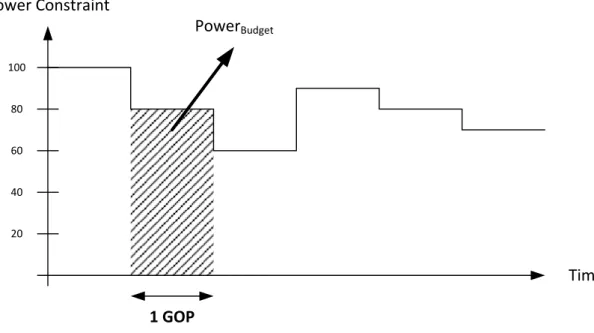
4.1. Concept of Power Constraint and Power Budget

As shown in Figure 4-1, we briefly introduce two basic concepts through the rest of this thesis, power constraint and power budget.

First, the concept of power constraint is a constraint on power consumption per MB of proposed power-aware encoder in order to have a power-aware environment. A power-aware environment is controlled according to various power conditions, such as different battery status, user preferences, and operating environments. Note that the power conditions do not change very often; say every frame or even every MB. Therefore, we choose the changing period of power constraint to be a Group of Picture (GOP).

Then, the concept of power budget denotes that the budget of power in one GOP can be allocated by proposed power-aware algorithm. It is shown as the shaded region in Figure 4-1. Before encoding of each GOP, we initialize the power budget defined in equation (4-1) according to three terms: MBsPerFrame, FramesPerGOP and PowerConstraint. The first two terms denote constant values, MB numbers per frame and frame numbers per second. The third term is power constraint mentioned before. After initialization of power budget, we enter the proposed MB level power allocation shown in Figure 4-2 until end of GOP.

(33)

18

Figure 4-1 power budget concept

(4-1)

Power Constraint Time 100 80 60 40 20 1 GOP PowerBudget

(34)

19

4.2. Overview of Proposed Algorithm

In order to meet the power constraint mentioned before while maximizing the rate-distortion performance, we develop a corresponding video encoding architecture which adaptively controls the power consumption of power-demanding part by the proposed algorithm shown in Figure 4-2.

Then, we analyze the encoding mechanism of our H.264 ASIC design in section 2.2.2. We know the dominant power-consuming parts in an H.264 encoder are ME and INTRA prediction (IP). The ME includes IME and FME. Therefore, a power-aware video encoding system focusing on ME and IP is a must.

To adaptively control the power consumption of ME and IP, we proposed four main parts which are colored with gray in Figure 4-2; skip mode detection, IME power allocation, FME power allocation, INTRA power allocation and power budget update. Details of each part are presented in the following sections. Note that we do not activate the proposed power-aware algorithm in I-frame because a poor quality I-frame may cause error propagating on the rest of P-frames in the same GOP.

(35)

20

Figure 4-2 flow chart of proposed power-aware algorithm

MB Start IME Power Allocation Skip ? IME FME Power Allocation INTRA Power Allocation FME FME ? INTRA MB End INTRA ? Mode Decision Loop Filter Entropy Skip Mode Detection IME ? Yes No INTRA frame ? Power Budget Update No Yes Yes No Yes Yes No No

(36)

21

4.3. Skip Mode Detection and IME Power Allocation

In this section, we present a skip mode detection and IME power allocation. There are two steps in the flow shown in Figure 4-3. First, we adopt a hardware friendly skip mode detection which is based on our previous work [16]. With the skip mode detection method, we can greatly reduce power consumption for our proposed power-aware algorithm. The power saved can be used for other un-coded and complex MBs which require more power to avoid quality degradation. Then, if the condition of skip mode detection is not met, we will go to IME power allocation marked with italic font. If left average power per MB obtained from equation (4-2) is larger than power of PowerOthers plus PowerIME both obtained from section 2.2.2, we

will allocate power to IME encoding, otherwise we allocate power to INTRA encoding only. In other words, we don’t use IME encoding to prevent power from being exhausted.

Figure 4-3 flow of skip mode decision and IME power allocation

(4-2)

(

1

)

1 1 − − − =

∑

− = k n Power Power Power k i i Usage Budget LeftAvg

(37)

22

4.4. Proposed FME Power Allocation

In this section, we present the proposed FME power allocation method in Figure 4-4. There two steps in the method. First, we first predict the power for FME encoding by the concept that MBs with larger IME minimum SAD cost have a larger opportunity to further reduce FME SATD cost significantly. Then we decide the power for FME encoding. In other words, we determine the number of modes for FME encoding. More details are as follow:

Figure 4-4 flow of FME power allocation

Step 1: FME Power Prediction

In this step, we develop a mechanism that can dynamically predict usable power for FME encoding of current MB according to available power budget. We present the predicted power of FME encoding for current MB (PowerPredFME) as in equation (4-3).

It is a product of two terms.

(4-3)

First term in the right hand side of equation (4-3) denotes left average power per MB for FME encoding (PowerLeftAvgFME), and it is defined in equation (4-4). In right

hand side of equation (4-4), PowerLeftAvg is obtained from equation (4-2); PowerOthers

and PowerIME are obtained from our power database in section 2.2.2. We use

⎟ ⎟ ⎠ ⎞ ⎜ ⎜ ⎝ ⎛ × = PreAvgIME CurMinIME LeftAvgFME PredFME SAD SAD Power Power

(38)

23

PowerLeftAvgFME to predict power for FME encoding, because we have no knowledge

about the future coding condition.

(4-4) Then, second term in the right hand side of equation (4-3) is the ratio of minimum IME SAD cost of current MB to average minimum IME SAD cost of previous MBs which is defined in equation (4-5). The idea of this term is to achieve the concept of allocating more power to FME encoding with larger IME SAD cost.

(4-5)

Step 2: FME Power Decision

After the predicted power for FME encoding obtained from step 1, we decide the power for FME encoding by considering the interval of FME power consumption shown in Figure 4-5. In which, Power1-mode FME and Power2-mode FME denote the power

consumption of 1-mode and 2-mode FME, and they are obtained from our power database in section 2.2.2.

Figure 4-5 power consumption of 1-mode and 2-mode FME

Then, the decision of the allocated power for FME encoding is shown blow. Note that the decision is only related to power concern.

PowerLeftAvgFME =PowerLeftAvg −

(

PowerOthers +PowerIME

)

NumPreIME SAD SAD 1 k 1 i i MinIME PreAvgIME

∑

− = =

(39)

24

if( PowerPredFME> Power2-mode FME)

{

2-mode FME; }

else if( PowerPredFME > Power1-mode FME) { 1-mode FME; } else { No FME; }

(40)

25

4.5. Proposed INTRA Power Allocation

In this section, we present an INTRA power allocation method to efficiently allocate power to INTRA-prone MB by a content-adaptive threshold. First, we introduce some observations and motivations. Then, the proposed INTRA power allocation flow is presented. Finally, we describe the most important part in the proposed algorithm, the threshold SADThd_INTRA4x4.

Three observations are presented here. First, the average percentage of MB which the final mode is INTRA is from 0.19% (low motion sequence, for example mobile) to 18.51% (high motion sequence, for example football). Thus, most power allocated to INTRA encoding is waste. If we can be sure at early stage that the best macroblock type belongs to INTER mode, we can bypass INTRA encoding stage and save lots of INTRA encoding power. Second, according to section 2.2.2, the INTRA encoding power is dominated by INTRA4x4 encoding power. Therefore, we choose to allocate INTRA4x4 encoding power in the proposed INTRA power algorithm, while INTRA16x16 encoding always turns on. Third, we observe most of best macroblock types belongs to the INTRA4x4 have large IME SAD cost. As a result, we can use the IME SAD cost to allocate INTRA encoding power. This observation is the main idea in the proposed content adaptive threshold in proposed INTRA power allocation.

The proposed INTRA power allocation algorithm is presented in Figure 4-6. First, we calculate the threshold SADThd_INTRA4x4 as equation (4-6). The details of the

threshold are in section 4.5.1. Then, if the IME minimum SAD cost of current MB is larger than SADThd_INTRA4x4, power will be allocated to INTRA4x4 encoding. In other

(41)

26

Figure 4-6 flow of INTRA power allocation

(4-6)

4.5.1. SAD

Thd_INTRA4x4

The SADThd_INTRA4x4 is a threshold used to decide whether turn on INTRA4x4

encoding or not. When the threshold is too low, too much power will be allocated to INTRA4x4 encoding, and other coding tools will have less power to use. Thus, the threshold plays an important role in tradeoff between power consumption and coding performance.

From equation (4-6), the threshold is a product of three terms. First term is the ratio of equation (4-7) to equation (4-8). This ratio is a good indication of INTRA MB probability among different sequences. For example, the ratio is 1.315 in INTRA-prone football sequence, while the ratio is 2.805 in non INTRA-prone mobile sequence. As a result, we choose the ratio to determine the threshold SADThd_INTRA4x4.

If the ratio is low, the proposed method tends to be INTRA-prone, and vice versa. Second term is the equation (4-5). It is average minimum IME SAD cost of previous MBs which can provide a reference level for threshold SADThd_INTRA4x4. Third part is a

weighting term which is a function of left average power per MB obtained from

(

)

LeftAvg PreAvgIME R PreAvgINTE A PreAvgINTR x4

Thd_INTRA4 SAD WeightPower

SATD SATD

(42)

27

equation (4-2). The function is shown in Table 4-1. We use an example to illustrate this viewpoint. In a power-rich environment, abundant power can be allocated to INTRA4x4 encoding for better quality, thus the threshold is low. On the contrary, in a low power environment, we have little power to allocate to INTRA4x4 encoding for better power distribution in the whole encoding system, thus the threshold is high.

(4-7)

(4-8)

Table 4-1 the SADThd_INTRA4x4 under different PowerLeftAvg

PowerLeftAvg [100,95) [95,90) [90,85) [85,80) [80,75) [75,70) [70,65) Others

Weighting 0.4 0.5 0.6 0.7 0.8 0.9 1.0 1.1

A NumPreINTR SATD SATD 1 k 1 i i MinINTRA A PreAvgINTR

∑

− = = R NumPreINTE SATD SATD 1 k 1 i i MinINTER R PreAvgINTE

∑

− = =

(43)

28

5. Simulation and Analysis

In this chapter, we present the simulation and analysis of our proposed algorithm mentioned in chapter 4. First, we will introduce the power constraint pattern. Then, we will present the experimental results in five categories as follows.

1. Rate-Distortion Performance 2. Power-Distortion Performance 3. Power Comparison

4. Distribution of skip mode 5. Distribution of INTRA MB

(44)

29

5.1. Power Constraint Pattern

We simulate the proposed algorithm with different power constraints. The definition of power constraint is presented in section 2.2.2. An example of constant power constraint of 80 is shown as a straight line in Figure 5-1, while another line is the power consumption of our proposed power-aware encoder. Note that we do not show the power consumption of first frame in each GOP due to its constant power consumption and simplicity of Figure 5-1. Though the proposed power-aware algorithm supports time-variant power constraint mentioned in section 2.2.2, we only present the simulation result of constant power constraint because the time variant one has similar result.

Figure 5-1 example of constant power constraint 80

0.00% 10.00% 20.00% 30.00% 40.00% 50.00% 60.00% 70.00% 80.00% 90.00% 100.00% 1 ₁₂ ₂₃ ₃₄ ₄₅ ₅₆ ₆₇ ₇₈ ₈₉ 100 111 122 133 144 155 166 177 188 199 210 221 232 Po w e r Frames Proposed Power constraint

(45)

30

5.2. Simulation Result

In this section, we present the simulation result of our proposed power-aware algorithm. At the beginning, there are two test schemes in our simulation, “PA without skip” and “PA with skip”. The “PA without skip” denotes the proposed power-aware algorithm without skip mode detection, while the “PA with skip” is our proposed one with skip mode detection.

In each of above test scheme, we will show the performance with four CIF size sequences, including low motion, medium motion and high motion. The low motion sequence is “Akiyo”, and the medium motion sequence is “Foreman”. The high motion sequences are “Football” and “Mobile”. Note that “Football” also has a large portion of INTRA-encoded MB.

The test settings are: baseline profile, no rate distortion optimization, one reference frame and no B frames are used. For simplicity, we set the number of frame per GOP to 10, and the leading frame of each GOP is an I-frame. We partition the simulation results to five categories mentioned before in order to evaluate the performance with different viewpoints. These categories are shown in the following section one by one.

(46)

31

5.2.1. Rate-Distortion Performance

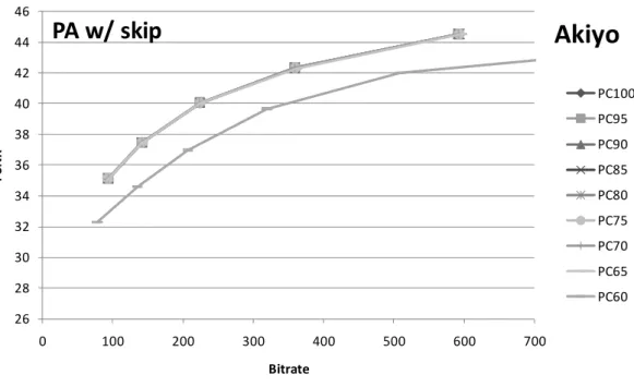
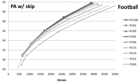
The RD curves for all test sequences under different power constraints are depicted from Figure 5-2 to Figure 5-9. Note that PC100 stands for power constraint of 100, and so on. These RD curves provide us a very first understanding of RD performance under different power constraints.

For low motion sequence in Figure 5-2 and Figure 5-3, we find that the two schemes both have nearly the same RD performance under power constraints of 70 and above. Besides, in scheme of “PA w/ skip”, we have a huge improvement on RD performance under power constraints of 65 and 60. Thus, we have a short conclusion that low motion sequence is suitable for low power constraint without degradation on RD performance especially when the skip mode detection is applied.

On the other hand, for median and high motion sequences in Figure 5-4 to Figure 5-9, there will be slight degradation on the RD performance when we increasingly lower the power constraint because the pre-skip rate is not as high as low motion sequence.

(47)

32

Figure 5-2 RD curves of PA w/o skip under different power constraints for “Akiyo”

Figure 5-3 RD curves of PA w/ skip under different power constraints for “Akiyo”

26 28 30 32 34 36 38 40 42 44 46 0 100 200 300 400 500 600 700 PS N R Bitrate

PA w/o skip

PC100 PC95 PC90 PC85 PC80 PC75 PC70 PC65 PC60

Akiyo

26 28 30 32 34 36 38 40 42 44 46 0 100 200 300 400 500 600 700 PS N R Bitrate

PA w/ skip

Akiyo

(48)

33

Figure 5-4 RD curves of PA w/o skip under different power constraints for “Foreman”

Figure 5-5 RD curves of PA w/ skip under different power constraints for “Foreman”

27 29 31 33 35 37 39 41 43 0 500 1000 1500 2000 2500 3000 PSN R Bitrate

PA w/o skip

Foreman

27 29 31 33 35 37 39 41 43 0 500 1000 1500 2000 2500 3000 PSN R Bitrate

PA w/ skip

Foreman

(49)

34

Figure 5-6 RD curves of PA w/o skip under different power constraints for “Football”

Figure 5-7 RD curves of PA w/ skip under different power constraints for “Football”

28 30 32 34 36 38 40 42 0 500 1000 1500 2000 2500 3000 3500 4000 4500 5000 PS N R Bitrate

PA w/o skip

Football

28 30 32 34 36 38 40 42 0 500 1000 1500 2000 2500 3000 3500 4000 4500 5000 PSNR Bitrate

PA w/ skip

Football

(50)

35

Figure 5-8 RD curves of PA w/ skip under different power constraints for “Mobile”

Figure 5-9 RD curves of PA w/ skip under different power constraints for “Mobile”

21 23 25 27 29 31 33 35 37 39 41 0 1000 2000 3000 4000 5000 6000 7000 PS N R Bitrate

PA w/o skip

Mobile

21 23 25 27 29 31 33 35 37 39 41 0 1000 2000 3000 4000 5000 6000 7000 PSNR Bitrate

PA w/ skip

Mobile

(51)

36

5.2.2. Power-Distortion Performance

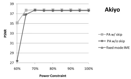
The power-distortion (PD) curve illustrated in Figure 5-10 shows the performance of a power-aware video coding system at a fixed bitrate. In Figure 5-10 between point A and point B, there are two power-aware curves, the solid one and the dashed one. The solid curve is the better one because the PSNR of point A is higher than the PSNR of point B at a fixed power constraint.

Thus, we analyze all the RD curves mentioned before with low, median and high bit rate, and depict PD curves in Figure 5-11 to Figure 5-22. Besides two test scheme mentioned before, we add one point in these curves. This point is called “fixed mode IME”, and is the non power-aware encoding with IME only. Because our proposed power-aware algorithm is mainly based on the result of IME, we check out how the PD curve of our proposed algorithm can approach this point.

In those PD curves, we find that average PSNR increase 6.5dB under the lowest power constraint 60 for low motion sequence when comparing power-aware with skip to power-aware without skip. For high motion sequence, we can also achieve the good PD curve as we mentioned before.

(52)

37

Figure 5-11 P-D curves of PA w/o skip and PA w/ skip for “Akiyo” at low bitrate 150(kb/s)

Figure 5-12 P-D curves of PA w/o skip and PA w/ skip for “Akiyo” at median bitrate 350(kb/s)

Figure 5-13 P-D curves of PA w/o skip and PA w/ skip for “Akiyo” at high bitrate 550(kb/s)

27 29 31 33 35 37 39 60% 70% 80% 90% 100% PS N R Power Constraint PA w/ skip PA w/o skip fixed mode IME

Akiyo

33 34 35 36 37 38 39 40 41 42 43 60% 70% 80% 90% 100% PS N R Power Constraint PA w/ skip PA w/o skip fixed mode IME

Akiyo

36 37 38 39 40 41 42 43 44 45 60% 70% 80% 90% 100% PS N R Power Constraint PA w/ skip PA w/o skip fixed mode IME

Akiyo

(53)

38

Figure 5-14 P-D curves of PA w/o skip and PA w/ skip for “Foreman” at low bitrate 400(kb/s)

Figure 5-15 P-D curves of PA w/o skip and PA w/ skip for “Foreman” at median bitrate 1300(kb/s)

Figure 5-16 P-D curves of PA w/o skip and PA w/ skip for “Foreman” at high bitrate 2200(kb/s)

28 29 30 31 32 33 34 35 60% 70% 80% 90% 100% PS N R Power Constraint PA w/ skip PA w/o skip fixed mode IME

Foreman

34 35 36 37 38 39 40 60% 70% 80% 90% 100% PS N R Power Constraint PA w/ skip PA w/o skip fixed mode IME

Foreman

37 38 39 40 41 42 60% 70% 80% 90% 100% PS N R Power Constraint PA w/ skip PA w/o skip fixed mode IME

Foreman

(54)

39

Figure 5-17 P-D curves of PA w/o skip and PA w/ skip for “Football” at low bitrate 1000(kb/s)

Figure 5-18 P-D curves of PA w/o skip and PA w/ skip for “Football” at median bitrate 2300(kb/s)

Figure 5-19 P-D curves of PA w/o skip and PA w/ skip for “Football” at high bitrate 3600(kb/s)

30.5 31 31.5 32 32.5 33 33.5 60% 70% 80% 90% 100% PS N R Power Constraint PA w/ skip PA w/o skip fixed mode IME

Football

35 35.5 36 36.5 37 37.5 38 38.5 60% 70% 80% 90% 100% PS N R Power Constraint PA w/ skip PA w/o skip fixed mode IME

Football

38 38.5 39 39.5 40 40.5 41 41.5 60% 70% 80% 90% 100% PS N R Power Constraint PA w/ skip PA w/o skip fixed mode IME

Football

(55)

40

Figure 5-20 P-D curves of PA w/o skip and PA w/ skip for “Mobile” at low bitrate 1200(kb/s)

Figure 5-21 P-D curves of PA w/o skip and PA w/ skip for “Mobile” at median bitrate 3300(kb/s)

Figure 5-22 P-D curves of PA w/o skip and PA w/ skip for “Mobile” at high bitrate 5400(kb/s)

22 23 24 25 26 27 28 29 30 31 60% 70% 80% 90% 100% PSN R Power Constraint PA w/ skip PA w/o skip fixed mode IME

Mobile

28 29 30 31 32 33 34 35 36 37 60% 70% 80% 90% 100% PSN R Power Constraint PA w/ skip PA w/o skip fixed mode IME

Mobile

33 34 35 36 37 38 39 40 41 60% 70% 80% 90% 100% PSN R Power Constraint PA w/ skip PA w/o skip fixed mode IME

Mobile

(56)

41

5.2.3. Power Comparison

We plot the curve of power constraint versus power consumption as shown in Figure 5-23 to Figure 5-26. There are five lines in those figures: “Ideal”, “PA w/o skip avg”, “PA w/ skip QP20”, “PA w/ skip QP28” and “PA w/ skip QP36”. The “Ideal” line means the maximum power consumption can be used. The “PA w/o skip avg” line stands for average of proposed power-aware algorithm without skip of all QPs. The others stand for proposed power-aware algorithm with skip of QP20, QP28 and QP36 individually. First, for the “PA w/o skip avg” line, we find that the power constraint is not exhausted when power constraints are 90 and 95. The power saved here is mainly from INTRA power allocation due to the saturated quality. In other words, increasing the power allocation to INTRA encoding only have little or no contribution to quality improvement. Then, we find the skip mode can save a lot of power for most test sequences especially for high QP.

(57)

42

Figure 5-23 power comparison of PA w/o skip and PA w/ skip for “Akiyo”

Figure 5-24 power comparison of PA w/o skip and PA w/ skip for “Foreman”

25% 35% 45% 55% 65% 75% 85% 95% 60% 65% 70% 75% 80% 85% 90% 95% Pow e r C ons um pt ion Power Constraint Ideal PA w/o skip avg PA w/ skip QP20 PA w/ skip QP28 PA w/ skip QP36

Akiyo

50% 55% 60% 65% 70% 75% 80% 85% 90% 95% 60% 65% 70% 75% 80% 85% 90% 95% Pow e r C o ns um pt ion Power Constraint Ideal PA w/o skip avg PA w/ skip QP20 PA w/ skip QP28 PA w/ skip QP36

Foreman

(58)

43

Figure 5-25 power comparison of PA w/o skip and PA w/ skip for “Football”

Figure 5-26 power comparison of PA w/o skip and PA w/ skip for “Mobile”

55% 60% 65% 70% 75% 80% 85% 90% 95% 60% 65% 70% 75% 80% 85% 90% 95% Pow e r C o ns um pt ion Power Constraint Ideal PA w/o skip avg PA w/ skip QP20 PA w/ skip QP28 PA w/ skip QP36

Football

55% 60% 65% 70% 75% 80% 85% 90% 95% 60% 65% 70% 75% 80% 85% 90% 95% Po w e r C ons um pt io n Power Constraint Ideal PA w/o skip avg PA w/ skip QP20 PA w/ skip QP28 PA w/ skip QP36

Mobile

(59)

44

5.2.4. Distribution of Skip Mode

From Figure 5-27 to Figure 5-34, we present the distribution of skip mode of our proposed algorithm with skip mode detection under different power constraints. In those figures, there are three kinds of skipped MB, one is “miss skip”, another is “correct skip”, and the other is “error skip”. First, the “miss skip” means that the MB should be pre-skipped but it is not detected in the pre-skip stage. Second, the “correct skip” represents that we successfully detect skip mode in the pre-skip stage. Third, the “error skip” denotes that the MB is pre-skipped but it should not be skipped. Because the skip mode distributions of three types mentioned above are similar under different power constraints of 65 and above, the average of those power constraints is presented in simulation result. Compare the skip mode distribution under power constraint of 65 and above to the skip mode distribution under power constraint 60, we find that the “correct skip” decreases under power constraint 60. Because a lot of MBs are only encoded with INTRA under power constraint 60, the MVP is not as accurate as power constraint of 65 and above.

(60)

45

Figure 5-27 skip mode distribution under power constraint from 95 to 65 for “Akiyo”

Figure 5-28 skip mode distribution under power constraint 60 for “Akiyo”

2.46% 2.58% 2.36% 1.85% 1.13% 59.95% 69.46% 74.91% 79.95% 84.24% 8.38% 5.96% 5.23% 4.71% 4.12% 29.21% 21.99% 17.50% 13.49% 10.51% 0% 10% 20% 30% 40% 50% 60% 70% 80% 90% 100% QP20 QP24 QP28 QP32 QP36 not skip miss skip correct skip error skip

Akiyo

PC95‐65

Akiyo

PC60

(61)

46

Figure 5-29 skip mode distribution under power constraint from 95 to 65 for “Foreman”

Figure 5-30 skip mode distribution under power constraint 60 for “Foreman”

Foreman

PC95‐65

Foreman

PC60

(62)

47

Figure 5-31 skip mode distribution under power constraint from 95 to 65 for “Football”

Figure 5-32 skip mode distribution under power constraint 60 for “Football”

Football

PC95‐65

Football

PC60

(63)

48

Figure 5-33 skip mode distribution under power constraint from 95 to 65 for “Mobile”

Figure 5-34 skip mode distribution under power constraint 60 for “Mobile”

Mobile

PC95‐65

Mobile

PC60

(64)

49

5.2.5. Distribution of INTRA MB

The Table 5-1, Table 5-2, Table 5-3 and Table 5-4 are the distribution of INTRA MB for two schemes mentioned before under different power constraints and sequences in QP28. There are four terms in these tables: “Allocated”, “Allocated INTRA”, “Original INTRA” and “Hitrate”. The “Allocated” means the percentage of MB which is allocated power to INTRA encoding by our proposed algorithm. The “Allocated INTRA” means the percentage of MB which final mode is INTRA when we allocate power to INTRA encoding. The “Original INTRA” means the minimum RD cost of the MB is INTRA. Note that in this condition we do not set final mode of the MB to INTRA when we do not allocate power to INTRA encoding. This term is only for hit rate analysis of INTRA distribution, and it is not feasible in hardware. The “Hitrate” is the ratio of “Allocated INTRA” to “Original INTRA”.

First, with all these tables, we find that our proposed algorithm tends to allocated more power to INTRA encoding when more INTRA-prone sequence is applied. For example, the sequence of football in Table 5-3 has the highest percentage of MB which power is allocated to INTRA encoding. Second, with non INTRA-prone

sequences of akiyo and mobile in Table 5-1 and Table 5-4, we will allocate less power to INTRA encoding. Third, we find that the results are similar in the two schemes in sequence of football, because high INTRA-prone sequence usually has low skip mode number.

(65)

50

Table 5-1 distribution of INTRA MB for PA w/o skip and PA w/ skip under different power constraints for “Akiyo” in QP28

Akiyo PA without skip PA with skip

QP28 Allocated (%) Allocated INTRA (%) Original INTRA (%) Hitrate (%) Allocated (%) Allocated INTRA (%) Original INTRA (%) Hitrate (%) PC95 30.38 0.00 0.00 100.00 17.38 0.00 0.00 100.00 PC90 22.53 0.00 0.00 100.00 17.10 0.00 0.00 100.00 PC85 14.33 0.00 0.00 100.00 16.47 0.00 0.00 100.00 PC80 7.32 0.00 0.00 100.00 15.54 0.00 0.00 100.00 PC75 5.23 0.00 0.00 100.00 14.56 0.00 0.00 100.00 PC70 4.03 0.00 0.00 100.00 13.60 0.00 0.00 100.00 PC65 3.43 0.00 0.00 100.00 12.74 0.00 0.00 100.00

Table 5-2 distribution of INTRA MB for PA w/o skip and PA w/ skip under different power constraints for “Foreman” in QP28

Foreman PA without skip PA with skip

Table 5-3 distribution of INTRA MB for PA w/o skip and PA w/ skip under different power constraints for “Football” in QP28

Football PA without skip PA with skip

(66)

51

Table 5-4 distribution of INTRA MB for PA w/o skip and PA w/ skip under different power constraints for “Mobile” in QP28

Mobile PA without skip PA with skip

(67)

52

6. Conclusion and Future Work

6.1. Conclusion

The main contribution of this thesis is to develop a power-aware video coding system suitable for the H.264 ASIC to maximize the rate-distortion performance while can dynamically meet different power constraints.

From our simulation, we know that the proposed method at 65% of power constraint can achieve nearly the same quality and bit rate as that in full power mode but only consumes 32.5% of full power for low motion sequences. On the other hand, for high motion sequences, the proposed method can degrade the quality gracefully for increasingly lower power supply, and achieves more than 1dB higher at PSNR compared with non power-aware scheme.

6.2. Future Work

In this thesis, we provide a good power-aware function, while there are several issues could be further analyzed to improve the performance of the power-rate-distortion performance. We can add more coding tools to the proposed power-aware H.264 encoder, such as high profile, level-1 IME and level-2 IME, in order to support high definition and high resolution video encoding on Digital Video (DV). A high resolution implies large search range. Thus, we can analyze some adaptive search range methods [19] [20] to have a balance between power and coding performance.

(68)

53

7. Reference

[1] Draft ITU-T Recommendation and Final Draft International Standard of Joint Video Specification (ITU-T Rec. H.264/ ISO/ IEC14496-10 AVC), Mar. 2003. [2] T. Wiegand, and et al, “Overview of the H.264/AVC Video Coding Standard,”

IEEE Transaction on Circuits and Systems for Video Technology, vol. 13, pp. 560-575, July 2003.

[3] T. Sakurai, “Perspectives on Power-Aware Electronics,” Digest of Technical Papers, IEEE Int. Solid-State Circuits Conf. 2003 (ISSCC 2003), vol. 1, pp. 26-29.

[4] L. G. Chen, “Power-aware multimedia,” SE2 Power-Aware Signal Processing, Evening Session, Digest of Technical Papers, IEEE International Solid-State Circuits Conference 2006 (ISSCC 2006), p. 17.

[5] M. Bhardwaj and et al, “Quantifying and enhancing power awareness of VLSI systems,” IEEE Trans. on Very Large Scale Integration (VLSI) Systems, vol. 9, no. 6, pp. 757–772, Dec. 2001.

[6] C. J. Lian and et al, “Power-Aware Multimedia: Concepts and Design Perspectives,” IEEE Circuits and Systems Magazine, vol. 7, issue 2, pp. 26-34, 2007.

[7] Z. HE and et al, “Power-Rate-Distortion Analysis for Wireless Video Communication Under Energy Constraints,” IEEE Transactions on Circuits and Systems for Video Technology, vol. 15, issue 5, pp. 645-658, May 2005.

[8] Z. HE and et al, “From rate-distortion analysis to resource-distortion analysis,” IEEE Circuits and Systems Magazine, vol. 5, no. 3, pp. 6-18, 2005.

(69)

54

[9] Y. H. Chen and et al, “Power-Scalable Algorithm and Reconfigurable Macro-Block Pipelining Architecture of H.264 Encoder for Mobile Application,” IEEE International Conference on Multimedia and Expo, pp. 281-284, July 2006.

[10] T. C. Chen and et al, “Low Power and Power Aware Fractional Motion Estimation of H.264/AVC for Mobile Applications,” in Proc. International Conference on Circuit and System (ISCAS), pp. 4, May 2006.

[11] S. S. Lin and et al, “Multi-Mode Content-Aware Motion Estimation Algorithm for Power-Aware Video Coding Systems,” in Proc. IEEE Workshop on Signal Processing Systems, pp. 239-244, 2004.

[12] T. C. Chen and et al, “2.8 to 67.2mW Low-Power and Power-Aware H.264 Encoder for Mobile Applications,” IEEE Symposium on VLSI Circuits, pp. 222-223, June 2007.

[13] H.264/MPEG 4 Part 10 White Paper, Overview, 2003.

[14] Y. K. Lin and et al, “A 242mW 10mm2 1080p H.264/AVC High Profile Encoder Chip,” International Solid-State Circuits Conference (ISSCC), pp. 314-315, Feb. 2008.

[15] Y. K. Lin and et al, “PMRME: A Parallel Multi-Resolution Motion Estimation Algorithm and Architecture for HDTV Sized H.264 Video Coding,” In proc. ICASSP, vol. 2, pp. 385-388, Apr. 2007.

[16] C. C. Lin and et al, “Hardware Efficient Skip Mode Detection for H.264/AVC,” International Conference on Consumer Electronics, pp. 1-2, Jan. 2008.

[17] Joint Video Team Reference Software JM9.0, ITU-T.

[18] Coding of Audio-Visual Objects – Part 2: Visual, ISO/IEC 14496-2, International Standard: 1999/Amd1:2000, Jan. 2000.

(70)

55

[19] Tian Song and et al, “Adaptive Search Range Motion Estimation Algorithm for H.264/AVC,” IEEE International Symposium on Circuits and Systems, pp. 3956-3959, May 2007.

[20] Toru YAMADA and et al, “Fast and Accurate Motion Estimation Algorithm by Adaptive Search Range and Shape Selection,” IEEE International Conference on Acoustics, Speech, and Signal Processing, vol. 2, pp. 897-900, March 2005.

適用於H.264視訊晶片之功率感知編碼系統

國 立 交 通 大 學

電子工程學系 電子研究所碩士班

碩 士 論 文

適用於 H.264 視訊晶片之功率感知編碼系統

Power-Aware Coding for H.264 Video Chip

研 究 生: 張瑋城

指導教授: 張添烜

適用於 H.264 視訊晶片之功率感知編碼系統

Power-Aware Coding for H.264 Video Chip

適用於 H.264 視訊晶片之功率感知編碼系統

摘要

Power-Aware Coding for H.264 Video Chip

Abstract

誌 謝

TABLE OF CONTENTS

LIST OF FIGURES

LIST OF TABLES

1. Introduction

1.1. Background

1.2. Related Work

1.3. Motivation and Contribution

1.4. Organization of the Thesis

2. Overview of H.264 Standard and Encoder Chip

2.1. Overview of H.264 Standard

2.1.1. Encoding Structure

2.1.2. Variable Block Size Motion Estimation

2.1.3. Quarter-Pixel Resolution Motion Vector

2.1.4. Directional Intra Prediction

2.1.5. In-Loop Deblocking Filter

2.1.6. Context Adaptive Entropy Coding

2.2. Overview of H.264 Encoder Chip

2.2.1. Overview of H.264 Encoder Chip

2.2.2. Power Consumption of H.264 Encoder Chip

3. Review of Power‐Aware Video Encoder

3.1. Review of Software‐Based Power‐Aware Video Encoder

3.2. Review of Hardware‐Based Power‐Aware Video Encoder

4. Proposed Hardware Oriented Power‐Aware

Algorithm

4.1. Concept of Power Constraint and Power Budget

4.2. Overview of Proposed Algorithm

4.3. Skip Mode Detection and IME Power Allocation

(

)

∑

4.4. Proposed FME Power Allocation

(

)

∑

4.5. Proposed INTRA Power Allocation

4.5.1. SAD

(

)

∑

∑

5. Simulation and Analysis

5.1. Power Constraint Pattern

5.2. Simulation Result

5.2.1. Rate-Distortion Performance

PA w/o skip

Akiyo

PA w/ skip

Akiyo

PA w/o skip

Foreman

PA w/ skip

Foreman

PA w/o skip

Football

PA w/ skip

Football

PA w/o skip

Mobile

PA w/ skip

Mobile

5.2.2. Power-Distortion Performance

Akiyo

Akiyo

Akiyo

Foreman

國立交通大學

電子工程學系電子研究所碩士班

碩士論文

研究生: 張瑋城

誌謝