Computer Simulation of 3D Temperature and Power Distributions in Tissue with a Countercurrent Blood Vessels Network during Hyperthermia

Computer Simulation of 3-D Temperature and Power

Distributions in Tissue with a Countercurrent

Blood Vessels Network during Hyperthermia

Huang-Wen Huang

Tzu-Ching Shih

Chihng-Tsung Liauh

Tzyy-Leng Horng

1_{Department of Innovative Information and Technology, Langyang Campus, Tamkang University, I-lan County 26247, Taiwan, ROC} 2_{Department of Biomedical Imaging and Radiological Science, China Medical University, Taichung 40402, Taiwan, ROC}

3

Department of Radiology, China Medical University Hospital, Taichung 40402, Taiwan, ROC

4_{Department of Mechanical Engineering, Kun Shan University, Tainan 71003, Taiwan, ROC} 5_{Department of Applied Mathematics, Feng Chia University, Taichung 40724, Taiwan, ROC}

Received 24 Mar 2009; Accepted 22 Jul 2009

Abstract

A countercurrent blood vessel network (CBVN) model for calculating tissue temperatures has been developed for studying optimized hyperthermia cancer treatment. This type of model represents a more fundamental approach to modeling temperatures in tissue than do the generally used approximate equations such as the Pennes’ bio-heat transfer equation (BHTE) or effective thermal conductivity equations. The 3-D temperature distributions are obtained by solving the conduction equation in the tissue and the convective energy equation with specified Nusselt number in the vessels. This study uses an optimization scheme to investigate the impact of thermally significant blood vessels during hyperthermia cancer treatment. The optimization scheme used here is adjusting power based on the local temperature in the treated region in an attempt to reach the ideal therapeutic temperature of 43ºC. The scheme can be used (or adapted) in a non-invasive power supply application such as high-intensity focused ultrasound (HIFU). Results show that first, a large amount of thermal absorbed power is focused on the locations near (or in) blood vessels and/or dense vessels in the treated tumor region during hyperthermia treatment as mass flow rates contribute cooling effects from vessels to tissues. Second, veins also play a significant role of affecting temperature distributions in the treated region and need to be taken into consideration.

Keywords: Hyperthermia, High Intensity Focused Ultrasound (HIFU), Optimization Power, Thermally Significant Vessels

1. Introduction

The Pennes’ [1] bio-heat transfer equation (BHTE) has been a standard model for predicting temperature distributions in living tissues for more than half century now. The equation was established through conducting a sequence of experiments of temperature measurements of tissue and arterial blood temperatures in the resting human forearm. The equation includes a special term that describes the heat exchange between blood flow and solid tissues. The blood temperature is assumed to be constant arterial blood temperature. Some researchers [2-6] also developed alternative equations having the same goal: to formulate a single, general field equation that can predict the overall characteristics of temperature * Corresponding author: Huang-Wen Huang

Tel: +886-3-9873088; Fax: +886-3-9873066 E-mail: hhw402@mail.tku.edu.tw

distributions in tissues. However, this has been challenged by many research groups internationally when trying to predict temperature distribution in regions which involving isolated large vessels.

Those approximate field equations neither have, nor were they ever intended to have, the ability to accurately model the effects of isolated, large vessels. Such infrequently occurring vessels cannot be simulated by such approximate field equations, which are intended to predict the average thermal behavior of the tissue. Thus, such vessels must be modeled using separate equations. The effect of such vessels have been studied by Chato [7] and Huang et al. [8,9], who developed analytical models for single vessels, and by other investigators [10-18] who have done numerical and experimental hyperthermia studies of single vessels and/or counter current vessel pairs imbedded in either a purely conductive media (with either a normal thermal conductivity, or an enhanced, effective thermal conductivity) or in media modeled by the Pennes

BHTE. One of those studies by Rawnsley et al. [17] compared the predictions from such a combined model (approximate field equation plus a separate blood vessel model) with experimental hyperthermia results. It clearly showed the increased accuracy of such combined models. Leeuwen et al. [18] also stressed that efforts to obtain information on the positions of the large vessels in an individual hyperthermia patient will be rewarded with a more accurate prediction of the temperature distribution. Finally a few studies have modeled the effect of collections of a large number of parallel vessels or of networks of vessels [18-21].

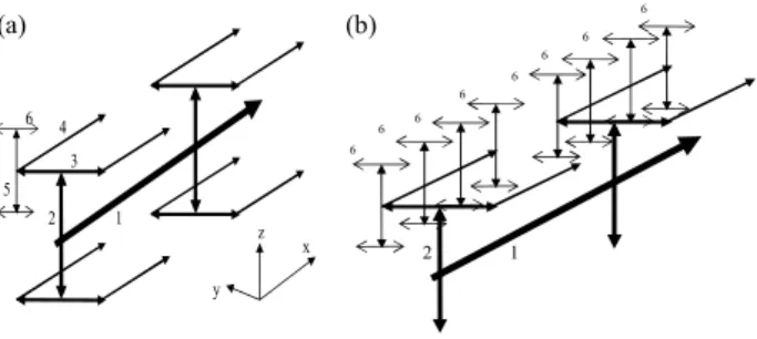
The present paper describes the effects of 3-D temperature distributions using a adapted model [19] comprising a network of blood vessels applied with an optimization scheme to reach ideal therapeutic temperature distribution of uniform 43ºC during hyperthermia cancer treatment. Figure 1 shows the constructed vascular model with vessel level generations up to level 6. This level 6 model presents no level 7 vessels and no blood perfusing linearly into tissues along the level 7 arteries. It gives an alternative to the one illustrated in the level 7 model [19]. This paper uses a rather simple, generic vessel network model in order to develop and illustrate the basic approach of the thermal model, and to illustrate the types of applications possible for such a model.

1 2 3 4 5 6 x z y 1 2 6 6 6 6 6 6 6 6

Figure 1. (a) The locations of a subset of the vessels in the whole control volume. All of the level 1, 2, 3 and 4 vessels are shown, but only two sets of the connected level 5-6 vessels are shown. A total of 64 such sets are used in the model, and they are regularly and uniformly spaced in the control volume. (b) The upper left hand quadrant of the entire blood vessel network. This quadrant contains 16 sets of the connected level 5-6 vessels. In total, there are 128 level 6 terminal vessels that pass through the centers of the 128 terminal subvolumes of Fig. 2 in [19].

2. Materials and methods

2.1 Vessel network geometry

The geometry used consists of a regular, branching vessel network as partially shown (only the arterial vessels are shown) in Figs. 1(a) and 1(b), that is embedded in a control volume which is an (approximate) cube of dimensions L = 8.2 cm and

W = H = 8 cm in the x, y, and z directions, respectively. All

vessels are straight line segments parallel to one of the three Cartesian axes. There are up to six levels of arteries, beginning with the main artery (level one) which lies along the central, lengthwise (x) axis of the cube. Table 1 of [19] lists the basic vessel network properties including level 7 vessels used in

these studies. The diameters of the arteries decrease by a constant ratio γ between successive levels of branched vessels (the ratio of diameters of successive vessel generations) i.e.

γ i1 i D D + = (1)

where Di and Di+1 are the diameters of two successive levels of

branching arteries. When two successive levels of numbered vessels do not branch but only change direction (i.e., levels six and seven in this model) the vessel diameter does not change.

The treated tumorous region is described by Fig. 2(a) with a volume of 2 cm by 2 cm by 2 cm in size. Inside the treated region, the locations and paths of arterial vessels are described in Figs. 2(b) and 2(c). The geometric arrangement of the countercurrent veins is essentially identical to that of the arteries, with all of the veins offset from the arteries by one finite difference node in x, y, and z as appropriate to avoid intersections of vessels. X=62 mm plane (x, y,z)= (0,40,40)mm X=0 plane X=42 mm plane (0,0,0) (42,40,40) (62,40,40) (62,40,60) (62,60,60) (62,20,40) (42,60,40) (42,60,60) (42,40,60) (a) (b) x z y 5 4 (c) 4 1 2 3 6 5 6 1 4 5 6 1 (62,60,60) (42,60,60) (52,60,60) (62,60,60) (52,60,60) (42,60,50)

Figure 2. (a) A transparent view of the parallelepiped showing the internal heated tumor region which is a cubic volume of 20 mm by 20 mm by 20 mm. The level 1 largest blood vessel is running through the volume’s edge from location (42, 40, 40) mm to location (62, 40, 40) mm. The original point is located at the southeastern corner when facing the x=0 plane. (b) The location of the cubic volume in a parallelepiped by indicating its 8 corners’ coordinates. The units are millimeters (mm). (c) A dissecting transparent view of all associated arterial blood vessel paths in the cubic volume. However veinous vessels do not appear in the figure. Within the volume, there are 2 branches of level 5-6 blood vessels, as the expanded dissecting view indicates. An x-y plane at z = 50 mm, shows multiples of level 6 arterial vessels.

2.2 Optimization scheme

The computational flow to continuously adjust power deposition in hyperthermia cancer treatment in order to reach ideal temperature (uniform temperature of 43°C throughout the volume of the tumorous region) is described below.

1. Set initial power field equal to 105 W/m3 uniform in the treated region.

2. Solve governing equations in tissue and blood temperature distributions with given boundary condition and inlet temperatures of vessels, which are all set to be 37 ºC. 3. Compare predicted temperature field with ideal temperature

field and calculate criteria value expressed below in Eq. (2). 4. If calculated temperature field does not meet the condition

described in Eq. (2), power is updated according to local temperature as it is described below in Eq. (4). Go to step 2 and continue the loop.

5. If calculated temperature field meets the condition, the optimal power and temperature distributions are obtained.

The criterion of power deposition theoretically can be based on two types of evaluation methods. The first method shown in Eq. (2), states that the root mean square of the difference between ideal temperature (which is set to be 43ºC) and calculated temperature in the treated region of all heated target nodes divided by (43-37)ºC reaches less than the criterion value (is set to be 10% of the temperature difference of (43-37)ºC). The second evaluation method, in Eq. (3), shows the average of the all magnitudes of temperature differences between ideal temperature (which is set to be 43ºC) and computational nodes (or tumor nodes) in the treated region. The value calculated in the second method is smaller than the value calculated in Eq. (2), which was chosen to perform our optimization scheme in this study. If the criterion is met, we have obtained the optimization of absorbed power such that the estimated temperature distribution is close to the ideal temperature distribution. Otherwise power deposition will be adjusted according to local temperature, i.e. it is a function of position and temperature. The readjusted power deposition is described in Eq. (4).

First evaluation method:

2

(43 37 )

( )

0.1

all target nodes

C

T

Total number of target nodes

T − °

∆

≤

∑

(2)

Second evaluation method:

(43 37 )

0.1

all target nodes

C

T

Total number of target nodes

T − ° ∆ ≤

∑

where ∆p(x, y, z) = Coef．∆T(x, y, z), Coef is 10000, n is the iteration index and ∆T(x, y, z) is the difference between ideal temperature (which is 43ºC) and calculated temperature. Smaller Coef values cause more repetitive loops in adjusting power deposition field to reach ideal temperature distribution. In other words, much more time is required to process the optimization. If the power deposited on a position that causes temperature in the tissue to rise over 43ºC, it will readjust its

power deposition to a smaller one in the scheme for an ideal temperature distribution.

2.3 Statistical analyses

The governing equation in tissues as described below, (k T x y z( , , )) w c T x y z_{b b}( ( , , ) T_a) q_s 0

∇ ∇ − _& − + =

(5) where k, cb, wb, and qs are the thermal conductivity of solid

tissue, specific heat of blood, blood perfusion rate and absorbed thermal power per volume in cubic meters from the source, respectively. The metabolism effect is neglected in Eq. (5).

The convective energy equation is solved for the CBVN model,

2 , ( , , ) ( ( , , ) ( , , )) ,

b i b b w b s bv i

m c∇T x y z =h⋅π T x y z −T x y z +qπR ( 6 ) where mb,i is the blood mass flow rate at level i vessel segment. h, Rbv,i and Tw are the heat transfer coefficient, thermal

conductivity in blood, the radius of blood vessel at level i and blood vessel wall temperature, respectively. The Nusselt number is defined as h/kb. A total of 682 vessels in the model

need to be calculated using Eq. (6). That is, i is from 1 to 682 for Eq. (6). Except for 128 arterial and 128 venous terminal ends of level 7 vessels, constant blood bleeding or collection along the vessels are considered.

2.4 Numerical methods

The numerical scheme used to calculate the temperatures was a black and red finite difference SOR method [22] with upwind differencing used for the vessels. The numerical details are described by Chen [23] and Huang [9]. Special algorithms are used to account for the vessel corners where arteries and veins change direction, and where two or more arteries divide, or two or more veins join. The thermal resistances around the circular vessels were calculated using the logarithmic resistance approach as described by Chen and Roemer [24]. The property values used in treated tumorous and non-treated normal tissues were k = 0.5 W/m3/ºC, c = cb = 4000 J/kg/ºC and ρ =

1000 kg/m3. The vessel heat transfer coefficient (h) was calculated using a constant Nusselt number of four (4) for all vessel levels. In all cases, a finite difference nodal spacing of 2mm was used. Test results with a nodal spacing of 1 mm for test cases using either the arterial vessel network (when no veins were present) or the countercurrent vessel network showed no significant differences with the results of the comparable 2-mm nodal spacing models. This 2-mm spacing gives an inter-vessel centerline to centerline diagonal spacing of 2.8 mm for the countercurrent vessels due to the 2-mm offsets in x, y, and z.

2.5Fully conjugated blood vessel network model or CBVN

CBVN model is a fully conjugated blood vessel network model. It is a model formulation which describes the solid tissue matrix having thermally significant vessel generations (six levels for level 6 model; seven levels for level 7 model). For terminal vessels, the blood perfuses into tissues provided with slow motion of liquid. Thermal equilibrium length is very

short for terminal vessels. The effects of all vessels smaller than the terminal vessels are not explicitly modeled in FCBVNM. Thus, those smaller vessels (connected to the terminal arteries and the terminal veins in the network) are implicitly assumed to be thermally insignificant in the FCBVNM. Details of the model are described in Huang et al. [19].

3. Results

Testing of this vascular network model has been done by several means [9] including: a check of the single-vessel numerical results (all vessels removed except the level one artery) against an analytical solution; a verification that all temperatures vary linearly with the applied power; and a check that for all results presented in this paper that the overall energy balance on the control volume was accurate to within 0.1 percent. In all cases studied in the present paper, the true tissue perfusion ( P

•

) was assumed to be uniform everywhere, i.e.,

i tsv P , • = P •

for I = 1-128 (The subscript tsv indicates terminal subvolume in the control volume.). Finally, Fig. 3 of [19] shows the vessel diameters, total surface areas, and velocity distributions (for P• = 0.5) as a function of the vessel level. The general trends present in that figure are similar to those shown for physiological systems in Green [25] and Whitmore [26].

(a) (b)

(c) (d)

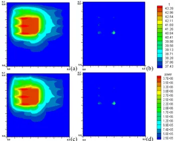
Figure 3. Temperature and absorbed power distributions at z = 50 mm, in the x-y plane of 82 mm by 80 mm in dimensions for perfusion rate of 0.5 kg·s-1m-3 after optimization. (x – vertical side, y – horizontal side) (a) temperature distribution at the x-y plane, which shows level 6 (terminal ends) arterial vessels in and out of treated tumorous region. (b) absorbed power distribution with the case (a). (c) temperature distribution in the x-y plane, which shows level 6-7 (terminal ends) arterial vessels in and out of the treated tumorous region with a vasculature with level 7 vessels present. (b) absorbed power distribution with case (c). (t: temperature units of ۫C, power: absorbed power units of W/m3).

The present vascular model with vessel level generations up to level 6 reveals no significant difference in temperature and power distributions (shown in Fig. 3) after optimization as

compared to a level 7 model which was used in 1996 for perfusion rate of 0.5 kg·s-1m-3 [19]. Fig. 3 shows temperature and absorbed power distributions at z = 50 mm, in an x-y plane of 82 mm by 80 mm in dimension for perfusion rate of 0.5 kg·s-1m-3 after optimization. (x – vertical side, y – horizontal side) Temperature distribution of Fig. 3(c) shows some perturbations due to the presence of level 7 arterial vessels as compared to Fig. 3(a) which indicates no level 7 arteries. As to power, a little bit more power for the level 7 model than the level 6 model is shown at the corners of Figs. 3(b) and (d). However it is negligible.

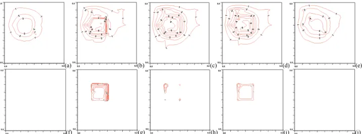
Unsuccessful hyperthermia treatments lead to survival of cancerous tissues. Insufficient net absorbed thermal energy in localized tissue area is one of the major problems. Figure 4(a) shows a cold spot at the center in which the spot is due to level 1 largest arterial blood vessel running perpendicularly inward to the plane. At its southeastern diagonal direction about 2.8 mm away to the level 1 artery, a level 1 veinous blood vessel is running in an opposite direction outward to the plane. The vein appears to be collecting some thermal energy by convection through the treated region as the vein’s temperature is higher than the artery’s. The plane of temperature distribution shown in Fig. 4(a) is approximately 40.0ºC near the treated region, which is located 4mm away from heated boundary.

Figure 4(b) shows steep thermal gradients near the level 2 artery running north from the center point, which is a branching node with level 1 artery. As shown in Fig. 4(g), large amount of thermal absorbed power were focused on level 2, 3 and 5 arteries after optimization. The maximum thermal absorbed power deposition is approximately 3.7E+6 W/m3. Figure 4(b) also shows that temperature higher than ideal temperature (which is 43ºC) exists outside of the treated region due to a level 6 westbound artery carrying convective thermal energy. Figure 4(c) shows maximum temperature located on (or near) the left-side artery branch node of level 5 and level 6 arteries in the treated region. Figure 4(h) shows large thermal power is focused on the corner of the treated region, an area having dense blood vessels (level 3, 4 and 5 arteries and veins).

Figure 4(d) shows the temperature distribution at the back boundary of the treated region and it’s surrounding. A cold spot is found near the northwestern corner of the heated region. The spot is 1.7ºC below the ideal temperature, and its cause is due to the level 4 vein flowing into the heated region. As expected, Fig. 4(i) shows a large amount of thermal energy is focused on the same corner shown in Fig. 4(h). Dense blood vessels in the area contribute to the effect of large amount of thermal power deposition.

Figure 4(e) shows some relative hot spots in the region which is 4 mm away from the back boundary of the heated volume. The hot spots are approximately 1ºC below the ideal temperature. One spot located in the northeastern direction that is more than 4 mm away from the region has a temperature of about 38.3ºC. Those hot spots are caused by arteries carrying more thermal away by convection, since the locations are downstream of arterial vessels to heated region.

There are, respectively, 6 levels of iso-temperature and iso-power contours shown in Figs. 4 and 5. From low to high

(a) (b) (c) (d) (e)

(f) (g) (h) (i) (j)

Figure 4. (a), (b), (c), (d) and (e) (top row from left to right) are temperature distributions at x=38 mm (4mm away from the front boundary), x=42 mm (the front boundary), x=52 mm (middle of the treated region), x=62 mm (the back boundary) and x= 66 mm (4mm away from the back boundary) planes respectively with perfusion rate of 0.5 kg·m-3_s-1 _{after power optimization scheme. The blood flow}

rate is about 320 mm/sec in the level 1 branch vessel. (f), (g), (h), (i) and (j) (bottom row from left to right) are thermal absorbed power distributions at x=38 mm (4mm away from the front boundary), x=42 mm (the front boundary), x=52 mm (the middle of the treated region), x=62 mm (the back boundary) and x= 66 mm (4mm away from the back boundary) planes, respectively, after power optimization scheme. No power is present on the planes at x=38 mm and 66 mm. There are 15 levels of iso-temperature and iso-power contours shown in the figures. From low to high 1-6 levels, the temperature (°C) set is {38, 39, 40, 41, 42, and 43} and the power (Wm-3_{) set is {2.5x10}5_{, 5.0x10}5_{, 1.0x10}6_{, 2.0x10}6_{, 3.0x10}6_{, and 3.5x10}6_{}, respectively.}

1-6 levels, the temperature (°C) set is {38, 39, 40, 41, 42 and 43}, and the power (Wm-3_{) set is {2.5x10}5_{, 5.0x10}5_{, 1.0x10}6_,

2.0x106_{, 3.0x10}6 _{and 3.5x10}6_}.

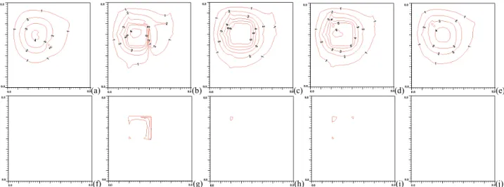
With perfusion rate reduced from 0.5 to 0.123 (kg·m-3_s-1_),

less thermal energy is removed by blood. As a result of this, power supply to the treated region is significantly reduced as shown in Figs. 5(g), (h) and (i). Comparing Fig. 5(g) to Fig. 4(g), the maximum thermal power deposition is about 7.7e5 to 3.7e6 Wm-3_{. The ratio is about 1 to 4.8 in reduction of}

power absorbed. Figures 5(a) and (e) show relatively higher temperatures in tissue as compared to Figs. 4(a) and (e). For example, at the location (38, 57, 23) mm, the tissue temperature is 37.96◦_{C for higher perfusion and 37.56ºC for the lower}

perfusion one.

From Figs. 5(b), (c) and (d), level 1, 2 and 3 vessels show still high thermal gradients near vessels. However, the level 5 and 6 vessels have significant reduced impact on local temperatures as the figures show rather smooth and uniform temperature distributions in the treated region. The level 1 artery passing by the edge of the treated region shows no significant impact on local temperature at downstream planes due to reduced mass flow rate and higher blood temperature in the vessel.

Figure 6 shows Temperature distributions of level 4 arterial (level4a) and veinous (level4v) vessel segments in and out of treated region from their downstream directions (x direction) for perfusion rate of 0.5 kg·m-3_s-1 _{at (x, y, z)}

= (x, 0.06, 0.06) meters. The association of level 4 vessel segments with treated region shows that the artery starts from the position 4.2 cm to 7.2 cm and its countercurrent vein starts from the reverse direction of the artery. Some portions of the temperature distribution are tissue temperatures, as indicated in the figure. Also, the distance between and artery and vein is about 2.8 mm. Boundary temperature is set to be 37°C.

4. Discussion and conclusion

The presented vascular model shown in Fig. 1 describes a level 6 model. The level 6 model shows no significant difference in temperature and power distributions with the level 7 model, as illustrated in Fig. 3. It implies that when in a low perfusion rate, the assumption of linear blood perfusion into tissues (via terminal vessels) acts as a way to connect to those vessels which are smaller than level 7 arteries. That means, it is an alternative model for the level 7 model under those conditions. The region perfused by a terminal vessel by the level 7 model is approximately a circle with radius of 1 cm, and the terminal vessel is located at center of circle. Slow motion of blood into tissues makes that reaching thermal equilibrium with tissues is in completion. Thus, the presence of level 7 vessels with optimization makes no significant difference in temperature with the level 6 model (removing level 7 vessels). Although there are temperature perturbations at the beginning spots of level 7 arteries, they are damped out very quickly in downstream direction.

From the simulation results, the CBVN model with γ = 0.9 and true perfusion rate of 0.5 and 0.123 kg·m-3s-1, temperature distributions show great impact by a network of vessels, particularly by level 1, 2 and 3 vessels. As optimization treatment is applied on the region with the CBVN model, the absorbed thermal power is focused on the region with thermally significant vessels which the vessels have large mass flow rates or the region contains high density of vessels. Veins also play a significant impact on temperature distributions at (or near) the treated boundary area. As shown in Figs. 6 and 4(d), the level 4 vein flows into the heated region from outside of the region, in which the outside region reserves a rather cold tissue temperature environment. From Figs. 4 and 5, mass flow rate and inlet vessel temperature of a vessel contribute vital factors in reaching uniform temperature distributions during hyperthermia.

(a) (b) (c) (d) (e)

(f) (g) (h) (i) (j)

Figure 5. (a), (b), (c), (d) and (e) (top row from left to right) are temperature distributions at x=38 mm (4mm away from the front boundary), x=42 mm (the front boundary), x=52 mm (the middle of the treated region), x=62 mm (the back boundary) and x= 66 mm (4mm away from the back boundary) planes respectively with perfusion rate of 0.123 kg·m-3s-1 after power optimization scheme. The blood flow rate is about 80 mm/sec in level 1 branch vessel. (f), (g), (h), (i) and (j) (bottom row from left to right) are thermal absorbed power distributions at x=38 mm (4mm away from the front boundary), x=42 mm (the front boundary), x=52 mm (the middle of the treated region), x=62 mm (the back boundary) and x= 66 mm (4mm away from the back boundary) planes respectively after power optimization scheme. No power presents on the planes at x=38 mm and 66 mm. There are 15 levels of iso-temperature and iso-power contours shown in figures. From low to high 1-6 levels, the temperature (℃) set is {38, 39, 40, 41, 42, and 43} and the power (Wm-3) set is {2.5x105, 5.0x105, 1.0x106, 2.0x106, 3.0x106, and 3.5x106}, respectively.

Figure 6. Temperature distributions of level 4 arterial (level4a) and veinous (level4v) vessel segments in and out of the treated region from their downstream directions (x direction) for perfusion rate of 0.5 kg·m-3s-1 at (x,y,z) = (x, 0.06, 0.06) meter. The association of level 4 vessel segments with the treated region shows that the artery starts from the position 4.2 cm to 7.2 cm and its countercurrent vein starts from the reverse direction of the artery. Some portions of the temperature distribution are tissue temperatures, as indicated in the figure.

In summary, the comparison of level 6 and level 7 models shows no significant difference in temperature and power distributions at a treated tumorous region when in a lower perfusion rate after optimization. Large amount of thermal absorbed power is focused on the locations near (or in) blood vessels and/or dense vessels in treated tumor region during hyperthermia treatment as mass flow rates contribute cooling effects from vessels to tissues. Also, veins are also playing a significant role in affecting temperature distributions in the treated region and need to be taken into consideration.

Future efforts should be aimed at developing more

accurate and tissue-specific fully conjugated models which can better predict actual tissue temperatures in in vivo situations. Acknowledgement

The authors would like to thank the National Science Council of Taiwan for partially supporting this research under no. NSC 98-2221-E-032 -033.

References

[1] H. H. Pennes, “Analysis of tissue and arterial blood temperature in the resting human forearm,” J. Appl. Phys., 1: 93-122, 1948. [2] M. M. Chen and K. R. Holmes, “Microvascular contributions in

tissue heat transfer,” Ann. NY Acad. Sci., 335: 137-150, 1980. [3] J. J. Lagendijk, M. Schellekens, J. Schipper and P M van der

Linden, “A three-dimensional description of heating patterns in vascularised tissues during hyperthermia treatment,” Phys. Med. Biol., 29: 495-507, 1984.

[4] S. Weinbaum and L. M. Jiji, “A new simplified bioheat equation for the effect of blood flow on local average tissue temperature,” J. Biomech. Eng.-Trans. ASME, 107: 131-139, 1985.

[5] J. J. Lagendijk and J. Mooibroek, “Hyperthermia treatment planning,” Recent Results Cancer Res., 101: 119-131, 1986. [6] L. M. Jiji, S. Weinbaum and D. E. Lemons, ‘Theory and

experiment for the effect of vascular microstructure on surface tissue heat transfer–Part II: Model formulation and solution,” J. Biomech. Eng.-Trans. ASME, 106: 331-341, 1984.

[7] J. C. Chato, “Heat transfer to blood vessels,” J. Biomech. Eng.-Trans. ASME, 102: 110-118, 1980.

[8] H. W. Huang, C. L. Chan and R. B. Roemer, “Analytical solutions of Pennes bio-heat transfer equation with a blood vessel,” J. Biomech. Eng.-Trans. ASME, 116: 208-212, 1994. [9] H. W. Huang, “Simulation of large vessels in hyperthermia

therapy,” Master’s Thesis, University of Arizona, Tucson, AZ, USA, 1992.

[10] J. W. Baish, “Heat transport by countercurrent blood vessels in the presence of an arbitrary temperature gradient,” J. Biomech. Eng.-Trans. ASME, 112: 207-211, 1990.

[11] J. W. Baish, P. S. Ayyaswamy and K. R. Foster, “Small-scale temperature fluctuations in perfused tissue during local hyperthermia,” J. Biomech. Eng.-Trans. ASME, 108: 246-250, 1986.

[12] J. W. Baish, P. S. Ayyaswamy and K. R. Foster, “Heat transport mechanisms in vascular tissues: a model comparison,” J. Biomech. Eng.-Trans. ASME, 108: 324-331, 1986.

[13] J. W. Baish, K. R. Foster and P. S. Ayyaswamy, “Perfused phantom models of microwave irradiated tissue,” J. Biomech. Eng.-Trans. ASME, 108: 239-245, 1986.

[14] C. K. Charny and R. L. Levin, “Heat transfer normal to paired arterioles and venules embedded in perfused tissue during hyperthermia,” J. Biomech. Eng.-Trans. ASME, 110: 277-282, 1988.

[15] Z. P. Chen and R. B. Roemer, “The effects of large blood vessels on temperature distributions during simulated hyperthermia,” J. Biomech. Eng.-Trans. ASME, 114: 473-481, 1992.

[16] J. Crezee and J. J. W. Lagendijk, “Experimental verification of bioheat transfer theories: measurement of temperature profiles around large artificial vessels in perfused tissues,” Phys. Med. Biol., 35: 905-923, 1990.

[17] R. J. Rawnsley, R. B. Roemer and A. W. Dutton, “The simulation of large vessel effects in experimental hyperthermia,” J. Biomech. Eng.-Trans. ASME, 116: 256-262, 1994.

[18] G. M. Van Leeuwen, A. N. Kotte, B. W. Raaymakers and J. J. W. Lagendijk, “Temperature simulations in tissue with a realistic

computer generated vessel network,” Phys. Med. Biol., 45: 1035-1049, 2000.

[19] H. W. Huang, Z. P. Chen and R. B. Roemer, “A counter current vascular network model of heat transfer in tissues,” J. Biomech. Eng.-Trans. ASME, 118: 120-129, 1996.

[20] D. Shrivastava and R. B. Roemer, “Readdressing the issue of thermally significant blood vessels using a countercurrent vessel network,” J. Biomech. Eng.-Trans. ASME, 128: 210-216, 2006. [21] J. W. Baish, “Formulation of a statistical model of heat transfer in

perfused tissue,” J. Biomech. Eng.-Trans. ASME, 116: 521-527, 1994.

[22] L. Lapidus and G. F. Pinder, Numerical Solution of Partial Differential Equations in Science and Engineering, New York: Wiley-Interscience Publication, 1982.

[23] Z. P. Chen, “A three-dimensional treatment planning program for hyperthermia,” PhD’s Dissertation, University of Arizona, Tucson, AZ, USA, 1989.

[24] Z. P. Chen and R. B. Roemer, “Improved Cartesian coordinate finite difference simulations of small cylindrical objects,” J. Biomech. Eng.-Trans. ASME, 115: 119-121, 1993.

[25] H. D. Green, “Circulation, physical principles,” in: O. Glasser (Ed.), Med. Phys., Chicago: The Year Book Publishers., 208-252, 1944.

[26] R. L. Whitmore, Rheology of the Circulation, New York: Pergamon Press, 1968.