Paper : TNN CE485
Data Classification with Radial Basis Function
Networks Based on a Novel Kernel Density Estimation
Algorithm
Yen-Jen Oyang∗, Shien-Ching Hwang1, Yu-Yen Ou2, Chien-Yu Chen3, and Zhi-Wei Chen4 Department of Computer Science and Information Engineering
National Taiwan University, Taipei, Taiwan, R. O. C. {yjoyang*, yien2, zwchen4}@csie.ntu.edu.tw
{schwang1, cychen3}@mars.csie.ntu.edu.tw
∗
Abstract
This paper presents a novel learning algorithm for efficient construction of the radial basis function (RBF) networks that can deliver the same level of accuracy as the support vector machines (SVM) in data classification applications. The proposed learning algorithm works by constructing one RBF sub-network to approximate the probability density function of each class of objects in the training data set. With respect to algorithm design, the main distinction of the proposed learning algorithm is the novel kernel density estimation algorithm that features an average time complexity of O(nlogn), where n is the number of samples in the training data set. One important advantage of the proposed learning algorithm, in comparison with the SVM, is that the proposed learning algorithm generally takes far less time to construct a data classifier with an optimized parameter setting. This feature is of significance for many contemporary applications, in particular, for those applications in which new objects are continuously added into an already large database.
Another desirable feature of the proposed learning algorithm is that the RBF network constructed is capable of carrying out data classification with more than two classes of objects in one single run. In other words, unlike SVM, it does not need to invoke mechanisms such as one-against-one or one-against-all for handling datasets with more than two classes of objects. The comparison with SVM is of particular interest, because it has been shown in a number of recent studies that SVM generally are able to deliver higher level of accuracy than the other existing data classification algorithms. As the proposed learning algorithm is instance-based, the data reduction issue is also addressed in this paper. One interesting observation in this regard is that, for all three data sets used in data reduction experiments, the number of training samples remaining after a naïve data reduction mechanism is applied is quite close to the number of support vectors identified by the SVM software. This paper also compares the performance of the RBF networks constructed with the proposed learning algorithm and those constructed with a conventional cluster-based learning algorithm. The most interesting observation learned is that, with respect to data classification, the distributions of training samples near the boundaries between different classes of objects carry more crucial information than the distributions of samples in the inner parts of the clusters.
Key terms: radial basis function (RBF) network, kernel density estimation, data classification,
1. Introduction
The radial basis function (RBF) network is a special type of neural networks with several distinctive features [21, 23, 27]. Since its first proposal, the RBF network has attracted a high degree of interest in research communities. A RBF network consists of three layers, namely the input layer, the hidden layer, and the output layer. The input layer broadcasts the coordinates of the input vector to each of the units in the hidden layer. Each unit in the hidden layer then produces an activation based on the associated radial basis function. Finally, each unit in the output layer computes a linear combination of the activations of the hidden units. How a RBF network reacts to a given input stimulus is completely determined by the activation functions associated with the hidden units and the weights associated with the links between the hidden layer and the output layer.
RBF networks have been exploited in many applications and quite a few learning algorithms have been proposed [5, 7, 8, 17, 19, 27, 29, 31, 32]. The problems that RBF networks have been applied to include function approximation, data classification, and data clustering. Depending on the problems that the learning algorithms are designed for, different optimization criteria may be employed.
One of the main applications that RBF networks have been applied to is data classification. However, latest development in data classification research has focused more on support vector machines (SVM) [13] than on RBF networks, because several recent studies have reported that SVM generally are able to deliver higher classification accuracy than the other existing data classification algorithms [16, 18, 20]. Nevertheless, SVM suffer one serious drawback. That is, the time taken to carry out model selection could be unacceptably long for some contemporary applications, in particular, for those applications in which new objects are continuously added into an already large database. Therefore, how to expedite the model selection process has become a critical issue for SVM and has been addressed by a number of recent articles [11, 14, 15, 22].
of SVM all lead to lower prediction accuracy. Anyway, this is an issue that deserves continuous investigation. Another minor drawback of SVM is that mechanisms such as one-against-one or one-against-all must be invoked to handle datasets with more than two classes of objects.
In this paper, a novel learning algorithm is proposed for efficient construction of the RBF networks that can deliver the same level of accuracy as SVM in data classification applications without suffering the drawbacks of SVM addressed above. In the RBF networks constructed with the proposed learning algorithm, each activation function associated with the hidden units is a spherical (or symmetrical) Gaussian function. In some articles, the specific type of RBF networks with spherical Gaussian functions is referred to as the spherical Gaussian RBF network [33]. For simplicity, we will use spherical Gaussian function (SGF) networks to refer to the RBF networks constructed with the learning algorithm proposed in this paper. With respect to algorithm design, the main distinction of the proposed learning algorithm is the novel kernel density estimation algorithm designed for efficient construction of the SGF network. The main properties of the proposed learning algorithm are summarized as follow:
(i) the SGF network constructed with the proposed learning algorithm generally delivers the same level of classification accuracy as the SVM;
(ii) the average time complexity for constructing an SGF network is bounded by O(n log n), where
n is total number of training samples;
(iii) the average time complexity for classifying n' incoming objects is bounded by O(n' log n). (iv) the SGF network is capable of carrying out data classification with more than two classes of
objects in one single run. That is, unlike the SVM, the SGF network does not need to incorporate mechanisms such as one-against-one or one-against-all for handling data sets with more than two classes of objects.
set in order to improve the efficiency of the instance-based classifier. Experimental results reveal that the naïve data reduction mechanism employed in this paper is able to reduce the size of the training data set substantially with a slight impact on classification accuracy. One interesting observation is that, in the three data sets used in experiments, the number of training samples remaining after data reduction is applied and the number of support vectors identified by the SVM software are in the same order. In fact, in two out of the three cases reported in this paper, the difference is less than 15%. Since data reduction is a crucial issue for instance-based learning algorithms, further study on this issue should be conducted.
This paper also compares the performance of the SGF networks constructed with the proposed learning algorithm and the RBF networks constructed with a conventional cluster-based learning algorithm [19]. The most interesting observation learned is that, with respect to data classification, the distributions of samples near the boundaries between different classes of objects carry more crucial information than the distributions of samples in the inner parts of the clusters. Since the conventional cluster-based learning algorithm for RBF networks places one radial basis function at the center of a cluster, the distributions of samples near the boundaries between different classes of objects may not be accurately modeled. As a result, the RBF network constructed with the conventional cluster-based learning algorithm in general is not able to deliver the same level of accuracy as those data classification algorithms such as SVM and the SGF network that exploit the distributions of samples near the boundaries between different classes of objects.
In the following part of this paper, section 2 presents a review of the related works. Section 3 presents an overview of how data classification is conducted with the proposed learning algorithm. Section 4 elaborates the novel kernel density estimation algorithm on which the proposed learning algorithm is based. Section 5 discusses the implementation issues and presents an analysis of time complexity. Section 6 reports the experiments conducted to evaluate the performance of the
2. Related Works
As mentioned earlier, there have been quite a few learning algorithms proposed for RBF networks. The learning algorithm determines the number of units in the hidden layer, the activation functions associated with the hidden units, and the weights associated with the links between the hidden and output layers. Learning algorithms designed for different applications may employ different optimization criteria. The general mathematical form of the output units in a RBF network is as follows:
∑
= = h i i j i j w r f 1 , ( ) ) (x x ) ,where f)j is the function corresponding to the j-th output unit and is a linear combination of h radial basis functions r1, r2, …, rh. Basically, there are two categories of learning algorithms
proposed for RBF networks [8, 27, 29]. The first category of learning algorithms simply places one radial basis function at each sample [28]. On the other hand, the second category of learning algorithms attempts to reduce the number of hidden units in the network, or equivalently the number of radial basis functions in the linear function above [12, 19, 24, 26, 25]. One primary motivation behind the design of the second category of algorithms is to improve the efficiency of the learning process, as the conventional approaches employed to figure out the optimal parameter settings for the RBF network involve computing the inverse of a matrix with dimension equal to the number of hidden units in the network.
As mentioned earlier, one of the main applications of RBF networks is data classification. Most learning algorithms proposed for constructing RBF network based classifiers conduct a clustering analysis on the training data set and allocate one hidden unit for each cluster [8, 17, 19, 25]. Algorithms differ by the clustering algorithm employed and how the parameters of the RBF network are set. The cluster-based approaches effectively improve the efficiency of the learning
cluster-based approaches typically place one radial basis function at the center of each cluster, the distributions of training samples near the boundaries between different classes of objects may not be accurately modeled. As the experimental results presented in section 6 of this paper reveals, with respect to data classification, the distributions of samples near the boundaries between different classes of objects carry more crucial information than the distributions of samples in the inner parts of the clusters. As a result, the RBF network constructed with a conventional cluster-based learning algorithm generally is not able to deliver the same level of accuracy as those data classification algorithms such as SVM and the SGF netowrk that exploit the distributions of samples near the boundaries between different classes of objects.
In this paper, a novel learning algorithm for constructing SGF networks is presented. The mathematical treatment presented in this paper for the derivation of the learning algorithm is different from our previous work []. Nevertheless, both treatments exploit essentially the same idea and result in the same equations.
3. Overview of Data Classification with the Proposed Learning Algorithm
This section presents an overview of how data classification is conducted with the SGF networks constructed with the proposed learning algorithm. The details of the learning algorithms will be elaborated in the next section.
Assume that the objects of concern are distributed in an m-dimensional vector space and let fj denote the probability density function that corresponds to the distribution of class-j objects in the
m-dimensional vector space. The proposed learning algorithm constructs one SGF sub-network
for approximating the probability density function of one class of objects in the training data set. In the construction of the SGF network, the learning algorithm places one spherical Gaussian function at each training sample. The general form of the SGF network based function approximators is as follows:
∑
∈ ⎟⎟⎠ ⎞ ⎜⎜ ⎝ ⎛− − = j S i i j w f i s i s v v 2 2 2 || || exp ) ( ˆ σ , (1) where(i) fˆ is the SGF network based function approximator for class-j training samples; j (ii) v is a vector in the m-dimensional vector space;
(iii) Sj is the set of class-j training samples;
(iv) ||v − si|| is the distance between vectors v and si;
(v) wi and σi are parameters to be set by the learning algorithm.
With the SGF network based function approximators, a new object located at v with unknown class is predicted to belong to the class that gives the maximum value of the likelihood function defined in the following:
) ( ˆ | | | | ) (v j j v j f S S L = ,
where Sj is the set of class-j training samples and S is the set of training samples of all classes. The essential issue of the learning algorithm is to construct the SGF network based function approximators. In the next section, the novel kernel density estimation algorithm designed for efficient construction of the SGF network will be presented. For the time being, let us address how to estimate the value of the probability density function at a training sample. Assume that the sampling density is sufficiently high. Then, by the law of large numbers in statistics [30], we can estimate the value of the probability density function fj(⋅) at a class-j sample si as follows:
1 2 1 ) 1 ( ) ( | | ) 1 ( ) ( 2 − ⎥ ⎥ ⎦ ⎤ ⎢ ⎢ ⎣ ⎡ + Γ ⋅ + ≅ m m j j m R S k f i π i s s (2) where
(ii) ) 1 ) ( 2 + ( Γ m2 m m R si π
is the volume of a hypersphere with radius R(si) in an m-dimensional vector
space;
(iii) Γ(⋅) is the Gamma function [1];
(iv) k1 is a parameter to be set either through cross validation or by the user.
In equation (2), R(si) is determined by one single training sample and therefore could be unreliable,
if the data set is noisy. In our implementation, we use R(si) defined in the following to replace
R(si) in equation (2), ⎟ ⎠ ⎞ ⎜ ⎝ ⎛ − + =
∑
= 1 1 1 || ˆ || 1 1 ) ( k h k m m R si sh si , where 1 2 1 s sksˆ ,ˆ ,...,ˆ are the k1 nearest training samples of the same class as si. The basis of
employing R(si) is elaborated in Appendix A.
4. The Proposed Kernel Density Estimation Algorithm
This section elaborates the efficient kernel density estimation algorithm for construction of the SGF network based function approximators. In fact, the proposed kernel density estimation algorithm is derived with some ideal assumptions. Therefore, some sort of adaptation must be employed, if the target data set does not conform to these assumptions. In this section, we will first focus on the derivation of the kernel density estimation algorithm, provided that these ideal assumptions are valid. The adaptation employed in this paper will be addressed later.
Assume that we now want to derive an approximate probability density function for the set of class-j training samples. The proposed kernel density estimation algorithm places one spherical Gaussian function at each sample as shown in equation (1). The challenge now is how to figure out the optimal wi and σi values of each Gaussian function. For a training sample si, the learning
set is derived from two ideal assumptions and serves as an analogy of the distribution of class-j training samples in the proximity of si. The first assumption is that the sampling density in the
proximity of si is sufficiently high and, as a result, the variation of the probability density function
at si and the neighboring class-j samples approaches 0. The second assumption is that si and the
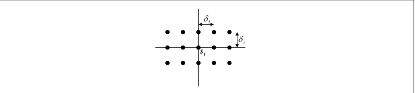
neighboring class-j samples are evenly spaced by a distance determined by the value of the probability density function at si. Fig. 1 shows an example of the synthesized data set for a
training sample in a 2-dimensional vector space. The details of the model are elaborated in the following.
(i) Sample si is located at the origin and the neighboring class-j samples are located at (h1δi,
h2δi, …, hmδi), where h1, h2, …, hm are integers and δi is the average distance between two
adjacent class-j training samples in the proximity of si. How δi is determined will be addressed later on.
(ii) The values of the probability density function at all the samples in the synthesized data set, including si, are all equal to fj(si). The value of fj(si) is estimated based on equation (2) in
section 3. i δ i δ i s
Fig. 1. An example of the synthesized data set for a training sample in a 2-dimensional vector space.
The proposed kernel density estimation algorithm begins with an analysis on the synthesized data set to figure out the values of wi and σi that make function gi(⋅) defined in the following
virtually a constant function equal to fj(si), ) ( 2 || ) ..., , , ( || exp ) ( 1 2 2 2 2 1 i s x x j h h h i i m i i i i f h h h w g m ≅ ⎥ ⎦ ⎤ ⎢ ⎣ ⎡ ⎟⎟ ⎠ ⎞ ⎜⎜ ⎝ ⎛− − =
∑ ∑ ∑
∞ −∞ = ∞ −∞ = ∞ −∞ = σ δ δ δ L . (3)In other words, the objective is to make gi(x) a good approximator of fj(x) in the proximity of si.
Let number real a is where , 2 ) ( exp ) ( 2 2 y h y y q h i i
∑
∞ −∞ = ⎟⎟⎠ ⎞ ⎜⎜ ⎝ ⎛ − − = σ δ . (4) Then, we have m R y i i m R y i q y g w q y w {Minimum[ ( )]} ( ) {Maximum[ ( )]} ∈ ∈ ≤ ≤ ⋅ ⋅ x , since∑ ∑ ∑
∞ −∞ = ∞ −∞ = ∞ −∞ = ⎟⎟⎠ ⎞ ⎜⎜ ⎝ ⎛ − − 1 2 2 2 2 1 2 || ) ..., , , ( || exp h h h i i m i i m h h h σ δ δ δ x L∑
∑
∑
∞ −∞ = ∞ −∞ = ∞ −∞ = ⎟⎟⎠ ⎞ ⎜⎜ ⎝ ⎛ − − ⋅⋅ ⋅ ⎟⎟ ⎠ ⎞ ⎜⎜ ⎝ ⎛ − − ⋅ ⎟⎟ ⎠ ⎞ ⎜⎜ ⎝ ⎛ − − = m h i i m m h i i h i i x h x h h x 2 2 2 2 2 2 2 2 1 1 2 ) ( exp 2 ) ( exp 2 ) ( exp 2 1 σ δ σ δ σ δ ,where x = (x1, x2, …, xm). It is shown in Appendix B that, if σi =δi, then q(y) is bound by
2.5066282745 ± 1.34 × 10⁻⁸. Therefore, with σi =δi, gi(x) defined in equation (3) is virtually a constant function. In fact, we can apply basically the same procedure presented in Appendix B to find the upper bounds and lower bounds of q(y) with alternative
i i
δ σ
ratios. As Table 1 reveals,
the bounds of q(y) becomes tighter, if
i i
δ σ
β = is set to a larger value. However, the tightness of the bounds of q(y) is not the only concern with respect to choosing the appropriate β value. We will discuss another effect to consider later.
i i δ σ β = Bounds of q(y) 0.5 1.253314144 ± 1.80 × 10⁻²
1.0 2.506628275 ± 1.34 × 10⁻⁸ 1.5 3.759942412 ± 2.94 × 10⁻¹¹
Tab. 1: The bounds of function q(y) defined in equation (4) with alternative i i
δ σ
ratios.
As it has been shown that, with an appropriate i
i
δ σ
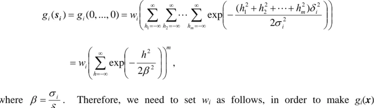
ratio, gi(x) defined in equation (3) is virtually a constant function, the next thing to do is to figure out the appropriate value of wi that makes equation (3) satisfied. We have
⎟ ⎟ ⎠ ⎞ ⎜ ⎜ ⎝ ⎛ ⎟⎟ ⎠ ⎞ ⎜⎜ ⎝ ⎛− + + + = =
∑
∞∑
∑
−∞ = ∞ −∞ = ∞ −∞ = 1 2 2 2 2 2 2 2 1 2 ) ( exp ) 0 ..., , 0 ( ) ( h h i i m h i i i m h h h w g g σ δ L L i s m h i h w ⎟⎟ ⎠ ⎞ ⎜ ⎜ ⎝ ⎛ ⎟ ⎟ ⎠ ⎞ ⎜ ⎜ ⎝ ⎛ − =∑
∞ −∞ = 2 2 2 exp β , where i i δ σβ = . Therefore, we need to set wi as follows, in order to make gi(x) a good approximator of fj(x) in the proximity of si:
) ( 2 exp 2 2 i s j m h i f h w ⎟⎟ = ⎠ ⎞ ⎜ ⎜ ⎝ ⎛ ⎟ ⎟ ⎠ ⎞ ⎜ ⎜ ⎝ ⎛ −
∑
∞ −∞ = β .If we employ equation (2) to estimate the value of fj(si), then we have
∑
∞ −∞ = 2 ⎟⎟ ⎠ ⎞ ⎜⎜ ⎝ ⎛ − = ⋅ ⋅ ⋅ + ( Γ ⋅ + = h m j m m i h R S k w m 2 2 1 2 exp where , ) ( | | ) 1 ) 1 ( 2 β λ π λ si . (7)So far, we have figured out that if we employ an appropriate ratio of i
i
δ σ
β = and set wi according to equation (7), we can make gi(x) a good approximator of fj(x) in the proximity of si.
The only remaining issue is to derive a closed form of σi. In this paper, δi is set to the average distance between two adjacent class-j training samples in the proximity of sample si. In an
m-dimensional vector space, the number of uniformly distributed samples, N, in a hypercube with
volume V can be computed by N Vm
α
Accordingly, we set m m i k R ) 1 ( ) 1 ( ) ( 2 1 + Γ + = π δ si , (8) where ⎟ ⎠ ⎞ ⎜ ⎝ ⎛ − + =
∑
= 1 1 1 || ˆ || 1 1 ) ( k h k m m R si sh si as defined in section 3.Finally, with equations (7) and (8) incorporated into equation (1), we have the following approximate probability density function for class-j training samples:
∑
∑
⎟⎟ ⎠ ⎞ ⎜⎜ ⎝ ⎛− − ⋅ ⋅ ⋅ + ( Γ ⋅ + = ⎟⎟ ⎠ ⎞ ⎜⎜ ⎝ ⎛− − = 2 ∈ i i s i i s i v s s s v v 2 2 1 2 2 2 || || exp ) ( | | ) 1 ) 1 ( 2 || || exp ) ( ˆ 2 i m j m m S i i j m j S R k w f σ π λ σ∑
∈ ⎟⎟⎠ ⎞ ⎜⎜ ⎝ ⎛− − ⎟⎟ ⎠ ⎞ ⎜⎜ ⎝ ⎛ ⋅ = j S i m i j S si i s v 2 2 2 || || exp | | 1 σ σ λ β , where (9)(i) v is a vector in the m-dimensional vector space, (ii) Sj is the set of class-j training samples,
(iii) m m i i k R ) 1 ( ) 1 ( ) ( 2 1+ Γ + = =βδ β π σ si , (iv)
∑
∞ −∞ = ⎟ ⎟ ⎠ ⎞ ⎜ ⎜ ⎝ ⎛ − = h h 2 2 2 exp β λ .In our study, we have observed that, regardless of the value of β, we have
β π β λ ⎟⎟≅ ⋅ ⎠ ⎞ ⎜ ⎜ ⎝ ⎛ − =
∑
∞ −∞ = 2 2 exp 2 2 h h. If this observation can be proved to be generally correct, then
we can further simplify equation (9) and obtain
∑
∈ ⎟⎟⎠ ⎞ ⎜⎜ ⎝ ⎛ − − ⎟⎟ ⎠ ⎞ ⎜⎜ ⎝ ⎛ ⋅ = j S i m i j j S f i s i s v v 2 2 2 || || exp 2 1 | | 1 ) ( ˆ σ σ π . (10)5. Implementation Issues and Analysis of Time Complexity
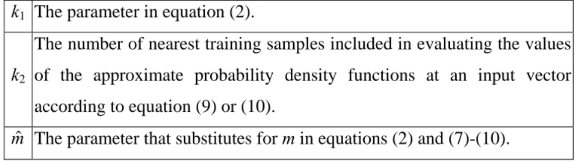
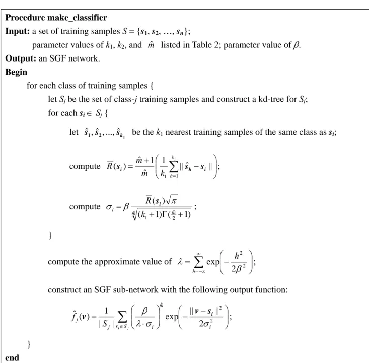
This section discusses the issues concerning implementation of the novel kernel density estimation algorithm proposed in the previous section and presents an analysis of time complexity. Fig. 2 summarizes the discussion so far by showing the detailed steps taken to create an SGF network based data classifier and how the SGF network works. In procedure make_classifier presented in Fig. 2, it is assumed that the optimal values of the three parameters listed in Table 2 have been determined through cross validation. In the later part of this section, we will examine the cross validation issue.
k1 The parameter in equation (2). k2
The number of nearest training samples included in evaluating the values of the approximate probability density functions at an input vector according to equation (9) or (10).
mˆ The parameter that substitutes for m in equations (2) and (7)-(10).
Table 2. The parameters to be set through cross validation for the SGF network.
With respect to the pseudo-codes presented in Fig. 2, there are several practical issues to address. The first issue concerns the two ideal assumptions on which the derivation of equations (9) and (10) is based, i.e. the assumptions from which Fig. 1 is derived. If the target data set does not conform to these assumptions, then some sort of adaptation must be employed. The practice employed in this paper is to incorporate parameter mˆ in Table 2. In equations (2) and (7)-(10), parameter m is supposed to be set to the number of attributes of the objects in the data set. However, because the local distributions of the training samples may not spread in all dimensions and some attributes may even be correlated, we replace m in these equations by mˆ, which is to be set through cross validation. In fact, the process conducted to figure out the optimal value of mˆ also serves to tune wi and σi, as we also replace m in equations (7) and (8) by mˆ.
Procedure make_classifier
Input: a set of training samples S = {s1, s2, …, sn};
parameter values of k1, k2, and mˆ listed in Table 2; parameter value of β.
Output: an SGF network.
Begin
for each class of training samples {
let Sj be the set of class-j training samples and construct a kd-tree for Sj; for each si ∈ Sj {
let
1 2
1 s sk
sˆ,ˆ ,...,ˆ be the k1 nearest training samples of the same class as si;
compute ⎟⎟ ⎠ ⎞ ⎜⎜ ⎝ ⎛ − + =
∑
= 1 1 1 || ˆ || 1 ˆ 1 ˆ ) ( k h k m m R si sh si ; compute m m i k R ˆ 2 ˆ 1 1) ( 1) ( ) ( + Γ + =β π σ si ; }compute the approximate value of
∑
∞ −∞ = ⎟⎟⎠ ⎞ ⎜⎜ ⎝ ⎛ − = h h 2 2 2 exp β λ ;
construct an SGF sub-network with the following output function:
∑
∈ ⎟⎟⎠ ⎞ ⎜⎜ ⎝ ⎛ − − ⎟⎟ ⎠ ⎞ ⎜⎜ ⎝ ⎛ ⋅ = j S i m i j j S f i s i s v v 2 2 ˆ 2 || || exp | | 1 ) ( ˆ σ σ λ β ; } endFig. 2. The pseudo codes of the proposed learning algorithm and the SGF network based classifier. (to be continued)
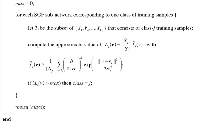
Procedure predict
Input: an SGF network constructed with the procedure presented in Procedure make_classifier; an input object with coordinate v;
Output: a prediction of the class of the input object;
Begin
max = 0;
for each SGF sub-network corresponding to one class of training samples { let Tj be the subset of {
2 2
1 s sk
sˆ ,ˆ ,...,ˆ } that consists of class-j training samples;
compute the approximate value of ˆ ( )
| | | | ) (v j j v j f S S L = with
∑
∈ ⎟⎟⎠ ⎞ ⎜⎜ ⎝ ⎛− − ⎟⎟ ⎠ ⎞ ⎜⎜ ⎝ ⎛ ⋅ ≅ j T i m i j j S f i s i s v v 2 2 ˆ 2 || || exp | | 1 ) ( ˆ σ σ λ β ;if (Lj(v) > max) then class = j; }
return (class);
end
Fig. 2. The pseudo codes of the proposed learning algorithm and the SGF network based classifier. (continues)
Another parameter in Table 2 and Fig. 2 that needs to address is k2. Since the influence of a
Gaussian function decreases exponentially as the distance increases, when computing the values of the approximate probability density functions at a given vector v according to equations (9) or (10), we only need to include a limited number of nearest training samples of v. The number of nearest training samples to be included can be determined through cross validation and is denoted by k2.
There is one more practical issue to address. In earlier discussion, we mentioned that there is another aspect to consider in selecting the
i i
δ σ
β = ratio, in addition to the tightness of the bounds of function q(y) defined in equation (4). If we examine equations (9) and (10), we will find that the value of the approximation function at a sample si, i.e. fˆj(si), is actually a weighted average
of the estimated sample densities at si and at its nearby samples of the same class. Therefore, a
suggests that, as long as β is set to a value within [0.6, 2], the value of β has no significant effect on classification accuracy. Therefore, β is not included in Table 2.
As far as the time complexities of the algorithms presented in Fig. 2 are concerned, there are two separate issues. The first issue concerns the time taken to create an SGF network with n training samples and the second issue concerns the time taken to classify n' objects with the SGF network. In both issues, we need to identify the nearest neighbors of a sample. In our implementation, the kd-tree structure is employed [6], which is a data structure widely used to search for the nearest neighbors. With this practice, the average time complexity for constructing a kd-tree with n training samples is O(n logn). In procedure make_classifier presented in Fig. 2, we need to construct c kd-trees, if the training data set contains c classes of samples. Therefore, the average time complexity of this task is bounded by O(cn logn). Then, we need to identify the
k1 nearest neighbors for each of the n training samples and the average time complexity of this task
is bounded by O(k1n logn). As the two tasks addressed above dominate the time complexity of
procedure make_classifier, the overall time complexity for the procedure is O(cn logn + k1n logn),
or O(n logn), if both c and k1 are regarded as constants.
In procedure predict presented in Fig. 2, the time complexity for classifying an incoming object is dominated by the work to identify k2 nearest training samples of the incoming object.
Therefore, the average time complexity for classifying one object is bounded by O(k2 logn) and
the overall time complexity for classifying n' incoming objects is bounded by O(k2n' log n) or O(n'
log n), if k2 is treated as a constant.
In the discussion above, it is assumed that the optimal values for the parameters listed in Table 2 have been determined through cross validation, before procedure make_classifier. If a k-fold cross validation process is conducted [35], then for each possible combination of parameter values we need to construct one SGF network based on a subset of training samples. Then, we need to invoke procedure predict to figure out how good this particular combination of parameter values is.
complexity of the cross validation process is bounded by O(n log n), if the number of possible combinations of parameter values is regarded as a constant.
6. Experimental Results and Discussions
The experiments reported in this section have been conducted to evaluate the performance of the SGF networks constructed with the learning algorithm proposed in this paper, in comparison with the alternative data classification algorithms. The experiments focus on the following 3 issues: classification accuracy, execution efficiency, and the effect of data reduction. The alternative data classification algorithms involved in the comparison include SVM, KNN [35], and the conventional cluster-based learning algorithm proposed in [19] for RBF networks. The learning algorithm proposed in [19] conducts clustering analysis on the training data set and allocates one hidden unit for each cluster of training samples. For simplicity, in the following discussion, we will use the conventional RBF network to refer to the data classifier constructed with the learning algorithm proposed in [19] and the SGF network to refer to the data classifier constructed with the learning algorithm proposed in this paper. In these experiments, the SVM software used is LIBSVM [10] with the radial basis kernel and the one-against-one practice has been adopted for the SVM, if the data set contains more than 2 classes of objects.
Data set # of training samples # of testing samples
satimage 4435 2000
letter 15000 5000
shuttle 43500 14500
(a). The three larger data sets.
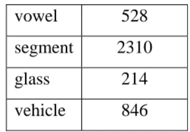
Data set # of samples
vowel 528
segment 2310
glass 214 vehicle 846 (b). The six smaller data sets.
Table 3. The benchmark data sets used in the experiments.
Table 3 lists main characteristics of the 9 benchmark data sets used in the experiments. All these data sets are from the UCI repository [9]. The collection of benchmark data sets is the same as that used in [18], except that DNA is not included. DNA is not included, because it contains categorical data and an extension of the proposed learning algorithm is yet to be developed for handling categorical data sets. Among the 9 data sets, three of them are considered as the larger ones, as each contains more than 5000 samples with separate training and testing subsets. The remaining six data sets are considered as the smaller ones and there are no separate training and testing subsets in these 6 smaller data sets. Accordingly, different evaluation practices have been employed for the smaller data sets and for the larger data sets. For the 3 larger data sets, 10-fold cross validation has been conducted on the training set to determine the optimal parameter values to be used in the testing phase. On the other hand, for the 6 smaller data sets, the evaluation practice employed in [18] has been adopted. With this practice, 10-fold cross validation has been conducted on the entire data set and the best result is reported. Therefore, the results reported with this practice just reveal the maximum accuracy that can be achieved, provided that a perfect cross validation mechanism is available to identify the optimal parameter values.
In these experiments, β in equation (9) has been set to 0.7. Our observation in this regard is that, as long as β is set to a value within [0.6, 2], then the value of β has no significant effect on classification accuracy. On the other hand, parameters α and β in the conventional RBF network
proposed in [19] have been set to the heuristic values suggested by the authors, i.e. 1.05 and 5, respectively.
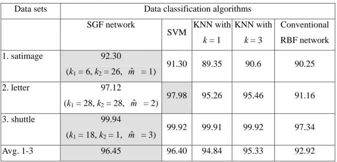
Data sets Data classification algorithms
SGF network SVM KNN with k = 1 KNN with k = 3 Conventional RBF network 1. satimage 92.30 (k1 = 6, k2 = 26, mˆ = 1) 91.30 89.35 90.6 90.25 2. letter 97.12 (k1 = 28, k2 = 28, mˆ = 2) 97.98 95.26 95.46 91.16 3. shuttle 99.94 (k1 = 18, k2 = 1, mˆ = 3) 99.92 99.91 99.92 97.34 Avg. 1-3 96.45 96.40 94.84 95.33 92.92
Table 4. Comparison of classification accuracy with the 3 larger data sets.
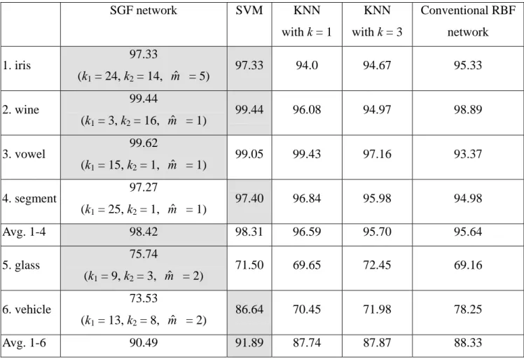
Table 4 compares the accuracy delivered by alternative classification algorithms with the 3 larger benchmark data sets. As Table 4 shows, the SGF network and the SVM basically deliver the same level of accuracy, which the KNN and the conventional RBF network are generally not able to match. Table 5 lists the experimental results with the 6 smaller data sets. Table 5 shows that the SGF network and the SVM basically deliver the same level of accuracy for 4 out of these 6 data sets. The two exceptions are glass and vehicle. The results with these two data sets suggest that both the SGF network and the SVM have some blind spots, and therefore may not be able to perform as well as the other in some cases. The experimental results presented in Table 5 also show that the SGF network and the SVM generally deliver a higher level of accuracy than the KNN and the conventional RBF network.
SGF network SVM KNN with k = 1 KNN with k = 3 Conventional RBF network 1. iris 97.33 (k1 = 24, k2 = 14, mˆ = 5) 97.33 94.0 94.67 95.33 2. wine 99.44 (k1 = 3, k2 = 16, mˆ = 1) 99.44 96.08 94.97 98.89 3. vowel 99.62 (k1 = 15, k2 = 1, mˆ = 1) 99.05 99.43 97.16 93.37 4. segment 97.27 (k1 = 25, k2 = 1, mˆ = 1) 97.40 96.84 95.98 94.98 Avg. 1-4 98.42 98.31 96.59 95.70 95.64 5. glass 75.74 (k1 = 9, k2 = 3, mˆ = 2) 71.50 69.65 72.45 69.16 6. vehicle 73.53 (k1 = 13, k2 = 8, mˆ = 2) 86.64 70.45 71.98 78.25 Avg. 1-6 90.49 91.89 87.74 87.87 88.33
Table 5. Comparison of classification accuracy with the 6 smaller data sets.
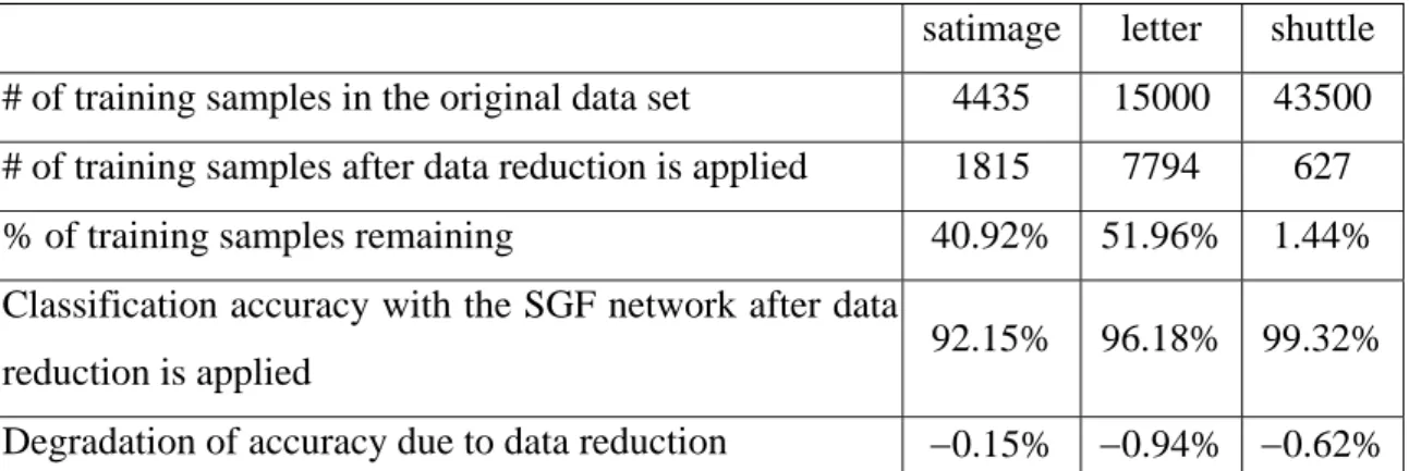
In the experiments that have been reported so far, no data reduction is performed in the construction of the SGF network. As the learning algorithm proposed in this paper places one spherical Gaussian function at each training sample, removal of redundant training samples means that the SGF network constructed will contain fewer hidden units and will operate more efficiently. Table 6 presents the effect of applying a naïve data reduction algorithm to the 3 larger data sets. The naïve data reduction algorithm examines the training samples one by one in an arbitrary order. If the training sample being examined and all of its 10 nearest neighbors in the remaining training data set belong to the same class, then the training sample being examined is considered as redundant and will be deleted. With this practice, training samples located near the boundaries between different classes of objects will be retained, while training samples located far away from the boundaries will be deleted. As shown in Table 6, the naïve data reduction algorithm is able to
reduce the number of training samples in the shuttle data set substantially, with less than 2% of training samples left. On the other hand, the reduction rates for satimage and letter are not as substantial. It is apparent that the reduction rate is determined by the characteristics of the data set. Table 6 also reveals that applying the naïve data reduction mechanism will lead to slightly lower classification accuracy. Since the data reduction mechanism employed in this paper is a naïve one, there is room for improvement with respect to both reduction rate and impact on classification accuracy. This is a subject under investigation.
satimage letter shuttle
# of training samples in the original data set 4435 15000 43500
# of training samples after data reduction is applied 1815 7794 627
% of training samples remaining 40.92% 51.96% 1.44%
Classification accuracy with the SGF network after data
reduction is applied 92.15% 96.18% 99.32%
Degradation of accuracy due to data reduction −0.15% −0.94% −0.62%
Table 6. Effects of applying a naïve data reduction mechanism.
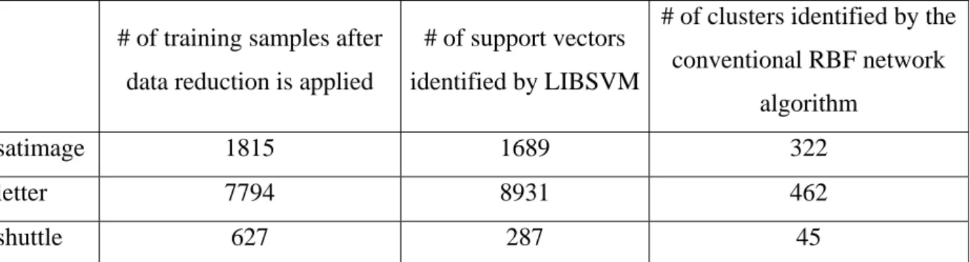
Table 7 compares the number of training samples remaining after data reduction is applied, the numbers of clusters identified by the conventional RBF network algorithm, and the number of support vectors identified by the SVM in the benchmark data sets. There are several interesting observations. First, for satimage and letter, the number of training samples remaining after data reduction is applied and the number of support vectors identified by the SVM are almost equal. For shuttle, though the difference is larger, the two numbers are still in the same order. On the other hand, the number of clusters identified by the conventional RBF network algorithm is consistently much smaller than the number of training samples remaining after data reduction is applied and the number of support vectors identified by the SVM. Our interpretation of these
to identify the training samples that are located near the boundaries between different classes of objects. Therefore, the numbers with these two algorithms presented in Table 7 are almost equal or at least in the same order. On the other hand, since multiple samples are needed to precisely describe the boundary of a cluster, the number of training samples remaining after data reduction is applied and the number of support vectors identified by the SVM are in general much larger than the number of clusters identified by the conventional RBF network algorithm. The results reported in Table 7 along with the results presented in Table 4 and Table 5 also suggest that, with respect to data classification, the distributions of samples near the boundaries between different classes of objects carry more crucial information than the distributions of samples in the inner part of the clusters. Since the conventional RBF network incorporates one radial basis function located at the geometric center of a cluster to model the distribution of the training samples inside the cluster, the accuracy delivered by the conventional RBF network is generally lower than that delivered by the SGF network and the SVM.
# of training samples after data reduction is applied
# of support vectors identified by LIBSVM
# of clusters identified by the conventional RBF network
algorithm
satimage 1815 1689 322
letter 7794 8931 462
shuttle 627 287 45
Table 7. Comparison of the number of training samples remaining after data reduction is applied, the number of support vectors identified by the SVM software, and the number of clusters
identified by the conventional RBF network algorithm.
Table 8 compares the execution times of the SGF network, the SVM, and the conventional RBF network with the 3 larger data sets presented in Table 3. In Table 8, the total times taken to construct classifiers based on the given training data sets are listed in the rows marked by
Make_classifier. On the other hand, the times taken by alternative classifiers to predict the classes of the testing samples are listed in the rows marked by Prediction.
SGF network without data reduction
SGF network with data
reduction SVM Conventional RBF network satimage 676 303 64644 136 letter 2842 1990 387096 712 Make classifier shuttle 98540 773 467955 2595 satimage 21.30 7.40 11.53 0.63 letter 128.60 51.74 94.91 2.15 Prediction shuttle 996.10 5.85 2.13 0.48
Table 8. Comparison of execution times in seconds.
As Table 8 reveals, the time taken to construct an SVM classifier with the model selection process employed in [10] is substantially higher than the time taken to construct an SGF network or a conventional RBF network. A detailed analysis reveals that it is the model selection process that dominates the time taken to construct an SVM classifier. These results imply that the time taken to construct an SVM classifier with optimized parameter setting could be unacceptably long for some contemporary applications, in particular, for those applications in which new objects are continuously added into an already large database.
The results in Table 8 also imply that, in dealing with those data sets such as satimage and
letter that does not contain a high percentage of redundant training samples, the SGF network is favorable over the SVM. In such cases, the SGF network enjoys substantially higher efficiency than the SVM in the make_classifier phase and is able to deliver the same level performance as the SVM in terms of both classification accuracy and the execution time in the prediction phase. On the other hand, if the data set contains a high percentage of redundant training samples such as
Prediction phase would suffer. With data reduction employed, the execution time of the SGF network in the Prediction phase then is comparable with that of the SVM. As the incorporation of the naïve data reduction mechanism may lead to slightly lower classification accuracy, it is of interest to develop advanced data reduction mechanisms.
Table 8 also shows that the conventional RBF network generally enjoys higher efficiency in comparison with the SGF network with data reduction and the SVM in the prediction phase. This phenomenon is due to the fact shown in Table 7 that the number of clusters identified by the conventional RBF network algorithm for a data set is generally smaller than the number of training samples employed to construct the SGF network after data reduction and the number of support vectors identified by the SVM algorithm. Nevertheless, as mentioned earlier, because the conventional cluster-based learning algorithm for RBF networks places one radial basis function at the center of each cluster, the distributions of the objects in the data set may not be accurately modeled. As a result, the conventional RBF network in general is not able to deliver the same level of accuracy as the SVM and the SGF network, which exploit the distributions of training samples near the boundaries between different classes of objects.
7. Conclusion
In this paper, a novel learning algorithm for constructing SGF network based data classifiers is proposed. With respect to algorithm design, the main distinction of the proposed learning algorithm is the novel kernel density estimation algorithm designed for efficient construction of the SGF networks. The experiments presented in this paper reveal that the SGF networks constructed with the proposed learning algorithm generally achieve the same level of classification accuracy as SVM. One important advantage of the proposed learning algorithm, in comparison with the SVM, is that the time taken to construct an SGF network with optimized parameter setting is normally much less that time taken to construct an SVM classifier. Another desirable feature of the SGF
single run. In other words, it does not need to invoke mechanisms such as one-against-one or one-against-all for handling datasets with more than two classes of objects. The other main properties of the proposed learning algorithm are as follow:
(i) the average time complexity for constructing an SGF network is bounded by O(n log n), where
n is total number of training samples;
(ii) the average time complexity for classifying n' incoming objects is bounded by O(n' log n).
As the SGF networks constructed with the proposed learning algorithm are instance-based, this paper also addresses the efficiency issue shared by almost all instance-based learning algorithms. Experimental results reveal that the naïve data reduction mechanism employed in this paper is able to reduce the size of the training data set substantially with a slight impact on classification accuracy. One interesting observation in this regard is that, for all three data sets used in data reduction experiments, the number of training samples remaining after data reduction is applied is quite close to the number of support vectors identified by the SVM software.
In summary, the SGF network constructed with the proposed learning algorithm is favorable over the SVM in dealing with a data set that does not contain a high percentage of redundant training samples. In such case, the SGF network is able to deliver the same level of performance as the SVM in terms of both accuracy and the time taken in the prediction phase, while requiring substantially less time to construct a classifier. On the other hand, if the data set contains a high percentage of redundant training samples, then data reduction must be applied, or the execution time of the SGF network would suffer. As the incorporation of the naïve data reduction mechanism may lead to slightly lower classification accuracy, it is of interest to develop advanced data reduction mechanisms. This paper also compares the performance of the SGF networks constructed with the proposed learning algorithm and the RBF networks constructed with a conventional cluster-based learning algorithm. The most interesting observation learned is that,
between different classes of objects carry more crucial information than the distributions of samples inside the clusters. As a result, the conventional RBF network generally is not able to deliver the same level of accuracy as those learning algorithms such as SVM and the SGF network that exploit the distributions of training samples near the boundaries between different classes of objects.
Based on the study presented in this paper, there are several issues that deserve further studies, in addition to the development of advanced data reduction mechanisms mentioned above. One issue is the extension of the proposed learning algorithm for handling categorical data sets. Another issue concerns why the SGF network fails to deliver comparable accuracy in the vehicle test case, what the blind spot is, and how improvements can be made. Finally, it is of interest to develop incremental version of the proposed learning algorithm to cope with the ever-growing contemporary databases.
Appendix A
Assume that 1 2 1 s sksˆ ,ˆ ,...,ˆ are the k1 nearest training samples of si that belongs to the same class
as si. If k1 is sufficiently large and the distribution of these k1 samples in the vector space is
uniform then we have
) 1 ( ) ( 2 1 2 + Γ ≈ m m m R k ρ si π ,
where ρ is the local density of samples
1 2
1 s sk
sˆ ,ˆ ,...,ˆ in the proximity of si. Furthermore, we have
∫
∑
⎟⎟ ⎠ ⎞ ⎜ ⎜ ⎝ ⎛ ( Γ ≈ − 2 − = ) ( 0 1 1 ) 2 || ˆ || 2 1 i m s R m m k h rdr r π ρ i h s s ) ( ) 1 ( ) ( 2 2 1 2 m m m R m Γ + = ρ si +π , where ) ( 2 2 1 2 m m m r Γ −πis the surface area of a hypersphere with radius r in an m-dimensional vector
∑
= − ⋅ + = 1 1 1 || ˆ || 1 1 ) ( k h k m m R si sh si .The right-hand side of the equation above is then employed in this paper to estimate R(si).
Appendix B
Let 2 ) ( exp ) ( 2 2∑
∞ −∞ = ⎟⎟⎠ ⎞ ⎜⎜ ⎝ ⎛ − − = h h y y q σ δ, where δ∈ R and σ∈ R are two coefficients and y ∈ R. We
have
(
)
∑
∞ −∞ = ⎟⎟⎠ ⎞ ⎜⎜ ⎝ ⎛− − − ⎟ ⎠ ⎞ ⎜ ⎝ ⎛− = = h h y h y dy y dq y q 2 2 2 2 ) ( exp 1 ) ( ) ( ' σ δ δ σ .Since q(y) is a symmetric and periodical function, if we want to find the global maximum and minimum values of q(y), we only need to analyze q(y) within interval [0 ,δ2]. Let y0 ∈ [0, 2
δ ) and =δ ⋅ +ε n j y 2
0 , where n ≥ 1 and 0 ≤ j ≤ n − 1 are integers, and 0 ≤ ε <
n 2 δ . We have
∫
+ + = δ δ ε δ n j n j q t dt q y q jn 2 2 ) ( ' ) ( ) ( 0 2 .Let us consider the special case with σ = δ. Then, we have
∑
∞∫
−∞ = + ⎥ ⎦ ⎤ ⎢ ⎣ ⎡ ⎟⎟ ⎠ ⎞ ⎜⎜ ⎝ ⎛− − − − ⎟ ⎠ ⎞ ⎜ ⎝ ⎛− − = h n j n j dt h t h t h n j y q ε δ δ σ δ δ σ 2 2 2 2 2 2 0 2 ) ( exp ) ( 1 ) 2 ( 2 1 exp ) ( . Let∫
+ ⎟⎟ ⎠ ⎞ ⎜⎜ ⎝ ⎛− − − − = δδ ε σ δ δ σ n j n j dt h t h t h r 2 2 2 2 2 2 ) ( exp ) ( 1 ) ( . Since ⎟⎟ ⎠ ⎞ ⎜⎜ ⎝ ⎛− − − − 2 2 2 2 ) ( exp ) ( 1 σ δ δ σ h t h t is adecreasing function for t ∈ [(h − 1)δ, (h + 1)δ] and is an increasing function for t ∉ [(h − 1)δ, (h + 1)δ], we have (i) ⎥ ⎥ ⎦ ⎤ ⎢ ⎢ ⎣ ⎡ ⎟ ⎠ ⎞ ⎜ ⎝ ⎛ − ⎟ ⎠ ⎞ ⎜ ⎝ ⎛ ⎟ ⎠ ⎞ ⎜ ⎝ ⎛ − ≤ 2 2 2 2 2 1 exp 2 1 ) 0 ( n j n j r δ σ δ σ ε ⎥ ⎥ ⎦ ⎤ ⎢ ⎢ ⎣ ⎡ ⎟ ⎠ ⎞ ⎜ ⎝ ⎛ − ⎟ ⎠ ⎞ ⎜ ⎝ ⎛ ⎟ ⎠ ⎞ ⎜ ⎝ ⎛ − = 2 2 2 1 exp 2 1 n j n j σ ε ; (ii) ≤ ⎛ −⎜ ⎞⎟⎜⎛ − ⎟⎞ ⎡⎢− ⎛⎜ − ⎞⎟ ⎥⎤ 2 1 exp 1 ) 1 ( ε jδ δ jδ δ r = ⎛ −⎜ ⎞⎟⎜⎛ − ⎟⎞ ⎡⎢− ⎛⎜ − ⎞⎟ ⎥⎤ 2 1 1 exp 1 1 j j ε ;
(iii) for h ≠ 0 and h ≠ 1, ⎥ ⎥ ⎦ ⎤ ⎢ ⎢ ⎣ ⎡ ⎟ ⎠ ⎞ ⎜ ⎝ ⎛ + − − ⎟ ⎠ ⎞ ⎜ ⎝ ⎛ + − ⎟ ⎠ ⎞ ⎜ ⎝ ⎛ − ≤ 2 2 2 2 ) 1 ( 2 1 exp 2 ) 1 ( 1 ) ( δ δ σ δ δ σ ε h n j h n j h r ⎥ ⎥ ⎦ ⎤ ⎢ ⎢ ⎣ ⎡ ⎟ ⎠ ⎞ ⎜ ⎝ ⎛ + − − ⎟ ⎠ ⎞ ⎜ ⎝ ⎛ + − ⎟ ⎠ ⎞ ⎜ ⎝ ⎛ − = 2 2 ) 1 ( 2 1 exp 2 ) 1 ( 1 h n j h n j σ ε . Therefore,
∑
∞ −∞ = ⎥⎦ ⎤ ⎢ ⎣ ⎡ + ⎟ ⎠ ⎞ ⎜ ⎝ ⎛− − = h h r h n j y q ) ( ) 2 ( 2 1 exp ) ( 0 2 ⎥+εθ ⎦ ⎤ ⎢ ⎣ ⎡ ⎟ ⎠ ⎞ ⎜ ⎝ ⎛− − ≤∑
∞ −∞ = h h n j 2 ) 2 ( 2 1 exp , where ⎥ ⎥ ⎦ ⎤ ⎢ ⎢ ⎣ ⎡ ⎟ ⎠ ⎞ ⎜ ⎝ ⎛ − − ⎟ ⎠ ⎞ ⎜ ⎝ ⎛ − ⎟ ⎠ ⎞ ⎜ ⎝ ⎛ − + ⎥ ⎥ ⎦ ⎤ ⎢ ⎢ ⎣ ⎡ ⎟ ⎠ ⎞ ⎜ ⎝ ⎛ − ⎟ ⎠ ⎞ ⎜ ⎝ ⎛ ⎟ ⎠ ⎞ ⎜ ⎝ ⎛ − = 2 2 1 2 2 1 exp 1 2 1 2 2 1 exp 2 1 n j n j n j n j σ σ θ∑
∞ ≠−∞ = ⎥ ⎥ ⎦ ⎤ ⎢ ⎢ ⎣ ⎡ ⎟ ⎠ ⎞ ⎜ ⎝ ⎛ + − − ⎟ ⎠ ⎞ ⎜ ⎝ ⎛ + − ⎟ ⎠ ⎞ ⎜ ⎝ ⎛ − + 1 , 0 2 2 ) 1 ( 2 1 exp 2 ) 1 ( 1 h h h n j h n j σ .If θ≥ 0, then we have for any
n 2 0≤ε < δ . 2 ) 2 ( 2 1 exp ) 2 ( 2 1 exp 2 εθ 2 δ θ n h n j h n j h h + ⎥ ⎦ ⎤ ⎢ ⎣ ⎡ ⎟ ⎠ ⎞ ⎜ ⎝ ⎛− − ≤ + ⎥ ⎦ ⎤ ⎢ ⎣ ⎡ ⎟ ⎠ ⎞ ⎜ ⎝ ⎛− −
∑
∑
∞ −∞ = ∞ −∞ = (A.1)On the other hand, if θ < 0, then we have for any
n 2 0≤ε< δ . ) 2 ( 2 1 exp ) 2 ( 2 1 exp 2 2 ⎥ ⎦ ⎤ ⎢ ⎣ ⎡ ⎟ ⎠ ⎞ ⎜ ⎝ ⎛− − ≤ + ⎥ ⎦ ⎤ ⎢ ⎣ ⎡ ⎟ ⎠ ⎞ ⎜ ⎝ ⎛− −
∑
∑
∞ −∞ = ∞ −∞ = h h h n j h n j εθ (A.2) Combining equations (A.1) and (A.2), we obtain, for all y ∈ [0, δ2),⎭ ⎬ ⎫ ⎩ ⎨ ⎧ + ⎟ ⎠ ⎞ ⎜ ⎝ ⎛− − ⎟ ⎠ ⎞ ⎜ ⎝ ⎛− − ≤
∑
∑
∞ −∞ = ∞ −∞ = − ≤ ≤ ∞ → θ δ n h n j h n j y q h h n n 2(2 ) 2 1 exp , ) 2 ( 2 1 exp Maximum lim ) ( 2 2 1 j 0 .Similarly, we can show that
⎭ ⎬ ⎫ ⎩ ⎨ ⎧ + ⎟ ⎠ ⎞ ⎜ ⎝ ⎛− − ⎟ ⎠ ⎞ ⎜ ⎝ ⎛− − ≥
∑
∑
∞ −∞ = ∞ −∞ = − ≤ ≤ ∞ → ρ δ n h n j h n j y q h h n n 2(2 ) 2 1 exp , ) 2 ( 2 1 exp Minimum lim ) ( 2 2 1 j 0 , where ⎥ ⎥ ⎦ ⎤ ⎢ ⎢ ⎣ ⎡ ⎟ ⎠ ⎞ ⎜ ⎝ ⎛ + − − ⎟ ⎠ ⎞ ⎜ ⎝ ⎛ + − ⎟ ⎠ ⎞ ⎜ ⎝ ⎛ − + ⎥ ⎥ ⎦ ⎤ ⎢ ⎢ ⎣ ⎡ ⎟ ⎠ ⎞ ⎜ ⎝ ⎛ + − ⎟ ⎠ ⎞ ⎜ ⎝ ⎛ + ⎟ ⎠ ⎞ ⎜ ⎝ ⎛ − = 2 2 1 2 1 2 1 exp 1 2 1 1 2 1 2 1 exp 2 1 1 n j n j n j n j σ σ ρ . 2 2 1 exp 2 1 1 , 0 2∑
∞ ≠−∞ = ⎥⎥⎦ ⎤ ⎢ ⎢ ⎣ ⎡ ⎟ ⎠ ⎞ ⎜ ⎝ ⎛ − − ⎟ ⎠ ⎞ ⎜ ⎝ ⎛ − ⎟ ⎠ ⎞ ⎜ ⎝ ⎛ − + h h h n j h n j σIf we set n = 100,000, then we have, with σ = δ,2.506628261≤q(y)≤2.506628288, for y ∈ [0,
2
δ ).
References
[1] E. Artin, The Gamma Function, New York, Holt, Rinehart, and Winston, 1964.
[2] R. K. Beatson, J. B. Cherrie, and C. T. Mouat, "Fast evaluation of radial basis functions: methods for four-dimensional polyhamonic splines," SIAM Journal on Scientific Computing, vol. 32. no. 6, pp. 1272-1310, 2001.
[3] R. K. Beatson and W. A. Light, "Fast evaluation of radial basis functions: method for two-dimensional polyharmonic splines," IMA Journal of Numerical Analysis, vol. 17, pp. 343-372, 1997.
[4] R. K. Beatson, W. A. Light, and S. Billings, "Fast solution of the radial basis function interpolation equations: domain decomposition methods," SIAM Journal on Scientific
Computing, vol. 22, no. 5, pp. 1717-1740, 2000.
[5] F. Belloir, A. Fache, and A. Billat, "A general approach to construct RBF net-based classifier," Proceedings of the 7th European Symposium on Artificial Neural Network, pp. 399-404, 1999.
[6] J. L. Bentley, "Multidimensional binary search trees used for associative searching,"
Communication of the ACM, vol. 18, no. 9, pp. 509-517, 1975.
[7] M. Bianchini, P. Frasconi, and M. Gori, "Learning without local minima in radial basis function networks," IEEE Transaction on Neural Networks, vol. 6, no. 3, pp. 749-756, 1995. [8] C. M. Bishop, "Improving the generalization properties of radial basis function neural
networks," Neural Computation, vol. 3, no. 4, pp. 579-588l, 1991.
[10] C. C. Chang and C. J. Lin, "LIBSVM: a library for support vector machines," http://www.csie.ntu. edu.tw/~cjlin/libsvm, 2001.
[11] O. Chapelle, V. Vapnik, O. Bousquet, and S. Mukherjee, "Choosing multiple parameters for support vector machines," Machine Learning, vol. 46, pp. 131-159, 2002.
[12] S. Chen, C. F. N. Cowan, and P. M. Grant, "Orthogonal least squares learning for radial basis function networks," IEEE Transactions on Neural Networks, vol. 2, no. 2, pp. 302-309, 1991. [13] N. Cristianini and J. Shawe-Taylor, An Introduction to Support Vector Machines, Cambridge
University Press, Cambridge, UK, 2000.
[14] D. Decoste and K. Wagstaff, "Alpha seeding for support vector machines," Proceedings of
International Conference on Knowledge Discovery and Data Mining, 2000.
[15] K. Duan, S. S. Keerthi, and A. N. Poo, "Evaluation of simple performance measures for tuning SVM hyperparameters," Neurocomputing, vol. 51, pp. 41-59, 2003.
[16] S. Dumais, J. Platt, and D. Heckerman, "Inductive learning algorithms and representations for text categorization," Proceedings of the International Conference on Information and
Knowledge Management, pp. 148-154, 1998.
[17] G. W. Flake, "Square unit augmented, radially extended, multilayer perceptrons," Neural
Networks: Tricks of the Trade, G. B. Orr and K. Müller, Eds., pp. 145-163, 1998.
[18] C. W. Hsu and C. J. Lin, "A comparison of methods for multi-class support vector machines," IEEE Transactions on Neural Networks, vol. 13, pp. 415-425, 2002.
[19] Y. S. Hwang and S. Y. Bang, "An efficient method to construct a radial basis function neural network classifier," Neural Networks, vol. 10, no. 8, pp. 1495-1503, 1997.
[20] T. Joachims, "Text categorization with support vector machines: learning with many relevant features," Proceedings of European Conference on Machine Learning, pp. 137-142, 1998. [21] V. Kecman, Learning and Soft Computing: Support Vector Machines, Neural Networks, and
[22] S. S. Keerthi, "Efficient tuning of SVM hyperparameters using radius/margin bound and iterative algorithms," IEEE Transactions on Neural Networks, vol. 13, pp. 1225-1229, 2002. [23] T. M. Mitchell, Machine Learning, McGraw-Hill, 1997.
[24] J. Moody and C. J. Darken, "Fast learning in networks of locally-tuned processing units,"
Neural Computation, vol. 1, pp. 281-294, 1989.
[25] M. Musavi, W. Ahmed, K. Chan, K. Faris, and D. Hummels, "On the training of radial basis function classifiers," Neural Networks, vol. 5, pp. 595-603, 1992.
[26] M. J. L. Orr, "Regularisation in the selection of radial basis function centres," Neural
Computation, vol. 7, no. 3, pp. 606-623, 1995.
[27] M. J. L. Orr, "Introduction to radial basis function networks," Technical report, Center for Cognitive Science, University of Edinburgh, 1996.
[28] M. J. Orr, "Optimising the widths of radial basis function," Proceedings of the Fifth Brazilian
Symposium on Neural Networks, 1998, pp. 26-29.
[29] M. J. Orr, J. Hallam, A. Murray, and T. Leonard, "Assessing rbf networks using delve,"
International Journal of Neural Systems, vol. 10, no. 5, pp. 397-415, 2000.
[30] A. Papoulis, Probability, Random Variables, and Stochastic Processes, McGraw-Hill, 1991. [31] T. Poggio and F. Girosi, "Networks for approximation and learning," Proceedings of the
IEEE, vol. 78, no. 9, pp. 1481-1497, 1990.
[32] M. J. Powell, "Radial basis functions for multivariable interpolation: a review," Algorithm for
Approximation, J. C. Mason and M. G. Cox, Eds, Oxford, U. K.: Oxford University Press,
1987, pp. 143-167.
[33] B. Scholkopf, K. K. Sung, C. Burges, F. Girosi, P. Niyogi, T. Poggio, and V. Vapnik, "Comparing support vector machines with Gaussian kernels to radial basis function classifiers," IEEE Transactions on Signal Processing, vol. 45, no. 11, pp. 1-8, 1997.