Gender differences in age at onset of schizophrenia

Numerous studies have indicated that male schizo

phrenic patients have an earlier age at onset than

females (Lewine, 1981; Eaton, 1985; Häfner,1987;

Angermeyer & Kuhn, 1988; Lewine, 1988; Goldstein

et al, 1989). This observation, along with other

fmdings, has led some to hypothesise that a biological

factor relating to gender may play a role in the onset

mechanism of schizophrenia (Seeman, 1983; DeLisi

eta!, 1989, 1991; Castle& Murray, 1991; Hafneret

a!, 1991). Although gender differences in age at onset

are among the most robust fmdings in schizophrenia

research (Wyatt et a!, 1988), the evidence from

previous studies must be interpreted cautiously due

to differences between the age distributions of male

and female patients.

The ages at onset observed in a series of patients

is biased by the underlying age distribution of the population (Crowe & Smouse, 1977; Heimbuch

et a!, 1980; Chen et a!, 1992b). If the age

distributions of males and females differs, then observed differences in age at onset could be artefactual. Since, in the general population, females tend to live longer than males, they are more likely

to surviveto - and hence suffer onset of disease at - a

laterage. Furthermore,the greatermortality for male

schizophrenic

patients exacerbates

this problem

(Goldstein et a!, 1992; Chen et a!, 1993). No

previous study of gender differences in age at onset

of schizophrenia have corrected this problem. So we

tested whether gender differences in the onset pattern

of schizophrenia would remain after applying

available methods of statistical correction (Chen et

a!, 1993).

Method

The subjects for this study came from two retrospective

cohort family studies. Details of the sample selection and

follow-upproceduresare describedelsewhere(Morrisonet

a!, 1972;Tsuang & Winokur, 1975). Briefly, probands

were selected from a blind review of index admission and

follow-up records and interviewsof 510 consecutive

admissionsto the Iowa PsychopathicHospital from 1934

to 1944witha chartdiagnosisof schizophrenia.Probands

wererediagnosedusing DSM-III (AmericanPsychiatric

Association, 1980) criteria by two expert psychiatrist diagnosticians (Kendler eta!, 1985). However, the criterion

limiting age at onset to 45 years was eliminated, as in

DSM-III—R

(AmericanPsychiatricAssociation, 1987).

Thestructured

interviewdevelopedbyTsuangci a!(1980)

collecteddiagnosticinformation about the probands. We

determined age at onset from all sources of information, including direct interviews, interviews with informants, and

medical charts (Kendler et a!, 1987). Age at onset was

defined as the age when psychoticsymptomsfirst became

evident. The reliability of this defmition was high, as

indicated by an intraclass correlation of 0.95 (Kendilerci

a!, 1987).

Outof orIginal510probands,therewere332DSM-III

schizophrenics. Among these schizophrenic probands, reliable data on age at onset were available for 319 patients.

The samplewasequallydividedbetweenmen (50.8%)and

women(49.2°!.).

For males,the durationbetweenage at

onset and age at admission ranged from 0 to 15 years with

a meanof 1.1and a standarddeviationof 2.4. For females,

these values ranged from 0 to 19 years with a mean of 1.4

and a standard deviation of 3.1. The difference between

males and females was not significant. Statistical procedures

To correctthe distributionof observedage at onset, we

applied the non-parametric method proposed by Baronet al (1983), with modifications to allow for increased

mortality after onset, which is the case for schizophrenia.

Our simulations indicate that the modified method

works effectively for this situation (Chen eta!, 1993). Four components of this methodology are essential for understanding our application to schizophrenia: (1) the relationship between age at onset and current age (or

625

Gender Differences in Age at Onset of Schizophrenia

STEPHENV. FARAONE,WEt J. CHEN, JILL M. GOLDSTEINand MING T. TSUANG

Numerousstudieshavefoundthat maleschizophrenicpatientshaveearlieragesat onsetthan females.However, noneof thesestudieshavecorrectedthe observedagesfor knowngender

differences

intheagedistribution

ofthepopulation.

Usinga pre-existing

dataset,we applied

a non-parametric

methodto correctthemaleandfemaledistributions

of observed

ageatonset

forsex-specific

agedistributions.

Thedistributions

of observedageat onsetindicatedearlier

onsetamongmales.Aftercorrection,

theage-at-onset

distributions

shiftedtowardolderages,

but the differencebetweenmalesandfemalesremainedstatisticallysignificant.Thus, gender

ageat ascertainment)whenascertainingfrom a seriesof prevalent cases; (2) the derivation of the age distribution for the susceptible population from which schizophrenic patients come; (3) the procedure for correcting an observed age at onset distribution; and (4) the method for comparing two corrected distributions.

The distribution of the observed age at onset is a function of two random variables: age at onset, X, and current age,

Y(Heimbuch eta!, 1980). We denote particular realisations

of these two random variables by x and y, respectively. When prevalent cases are sampled, the observed age at onset distribution is conditional on X being less than V. Assume

that F(x) =p(Xx) is the true age at onset distribution

which we are trying to estimate, C(y) =p( Yy) is the age distribution of the susceptible population, and

H(x) =p(Xx@X Y) is the observed age at onset distribution. The corresponding density functions of these

three distributions are f(x), c(y), and h(x), respectively.

If the illness has negligible effects on mortality and fertility, then the age distribution of the susceptible

population, C(y), is the same as that of the general population. The relationship between true and observed age

at onset distributions is as follows (Baron et a!, 1983):

h(x) = -@-f(x)[I —¿C(x) J. (I)

K is a normalising constant to make the integral of h

equal to one. A key feature of equation (1) is that 1(x) is multiplied by the age distribution beyond age at onset x,

[I —¿C(x)], while a subject's current age, y, is not directly

reflected in the formula. Thus, the cumulative age distribution, C(y), is evaluated at the age of onset, x. A common way to obtain C(y) is to assume that the population is in equilibrium (Cavalli-Sforza & Bodmer, 1971). Assuming !(y) is the survival distribution function

up to agey (i.e., the probability that an individual will not die before reaching age y) and r is the intrinsic rate of

natural growth in the population, then the density function for the age distribution C(y) is:

c(y) = n1(y)e@

where n is a normalising constant to make the integral of c equal to one. Both 1(y) and r can be obtained from vital statistics.

However, because the mortality rate of schizophrenic patients is increased after onset, the age distribution of the susceptible population is no longer the same as that of the general population. Instead, the current age, Y, becomes dependent on the age at onset, X. We denote the conditional age distribution as D(y(x) =p( Yy@X=x) and its density function as d(ylx). Then the density function of the observed age at onset distribution becomes:

h(x)=j@/(x) [l—D(xlx)] (3)

For convenience, we divide both age at onset and age into 18 discrete intervals denoted x, and y., respectively. We then assume that the age distribution of subjects in each onset interval is in equilibrium with its specific survivorship function.Modified from equation (2),the conditionalage distribution for subjects whose onset occurred in the ith

interval, x,, is:

d(yIx1)=nm(yIx,)e@

where n is a normalising constant to make the integral of

d equal to one, and m(y@x,)=p(Yy@X=x1) is the

survivorship function for subjects whose age at onset is x1. Having derived equations (3) and (4), the remaining information we must provide to obtain a corrected distribution of age at onset is the conditional survivorship

function for schizophrenic patients, m(y@x1). As we have

demonstrated elsewhere (Chen et a!, l992a; Chen et a!,

1993), we can apply the standardised mortality ratio of

schizophrenic patients to model their conditional mortality rates as follows. Starting with data from the life table for the general population, we first multiply the number of deaths belonging to intervals that are greater than the age at onset x1 by the standardised mortality ratio, denoted as a. We then derive the new survivorship functions in each interval by subtracting the newly calculated number of deaths from the number alive in the previous interval. For

age y1, j= 1 to 18, the new survivorship function is

calculated as follows:

=I(y,)—(a— 1)(k@.tyk/1OO0OO) for x1<y@and the

- item0

(5)

=0 otherwise

where t@.is the number of deaths in the age interval y@. Thus, based on equation (5), we can compute the

conditional survivorship function for schizophrenic patients

if we specify the standardised mortality ratio, a, and the (2@ survivorship function of the general population, 1(y1).

Comparing the mortality rates of the schizophrenic

probands used in this study to that of the general

population, Tsuang & Woolsen (1977) reported that the

standardised mortality ratios in the first, second, third, and

fourth decades after admission were 4.69, 3.40, 0.86 and 1.44 for males and 3.30, 1.30, 2.06 and 1.80 for females. Because the mean (s.d.) duration between age at onset and age at admission (1.1 (2.4) years for males and 1.4 (3.1) years for females) is less than the length of a single 5-year interval, we use these four values as the standardised mortality ratio, a, to represent the increased mortality rates for four different lengths of time after onset. After the

conditional survivorship function for schizophrenic patients

is calculated according to equation (5), we then use equation (4) to compute their conditional age distribution. Because we did not have the intrinsic rate of natural increase, r, for the Iowa population in 1940, we chose three values based on national data (0.001 for all races, 0.0001 for white, and 0.0074 for all other).

m(y1lx,)=I(y@) for

To estimate the underlying true age at onset distribution,

Age@at-onset

distributionsMale (n=162)

Means.d.Female

In =157) Mean s.d.Two-distribution x2 test x2 (d.f.=6)' PObserved24.3 6.128.0 8.326.2 <0.0001Correctedr=0.000126.2 7.131.1 9.928.3 <0.0001r=0.001026.2 7.131.1 9.928.4 <0.0001r=0.007426.4 7.131.5 10.129.2 <0.0001

GENDER DIFFERENCES IN AGE AT ONSET OF SCHIZOPHRENIA

Afterbeingadjustedfor the underlyingage distributions,

the corrected distributions move toward older ages as

compared with the observed ones. The means and standard

deviationsof the observedand correctedage at onset

distributions

aresummarised

in TableI. Beforecorrection,

the male distributionis significantlyyounger than the

female one, accordingto the two-distributionx1 test.

After correction, the male distributions are still significantly

different from the females, regardlessof which r is used

in the adjustment.In fact, for all threevaluesof r, the

means and standard deviations of the corrected distributions

are similar.

Discussion

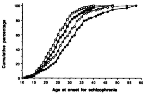
As predicted, the distribution of the observed age

at onset of schizophrenia is biased toward younger

ages. As shown in Fig. 1, only 5.6% of males and

18.5% of females have observed ages at onset greater

than 35 years. After correction, these percentages

increase to! 1.8% and 30.1%, respectively. The non negligible downward biases in the observed age at

onset distributions is consistent with the pattern

demonstrated

in simulation studies (Chen et a!,

1993).

However, although the observed ages at onset for

male and female schizophrenics are biased, we also

show that the observed gender differences are not

spurious. Through our non-parametric method, we

controlled for three potential confounders in the

comparison: the age composition of the population

of origin, excess mortality among schizophrenic

patients, and the gender differences in mortality

among these patients.

Nevertheless, our results may be limited by the

assumptions

required

in our derivation

of the

corrected age at onset distribution. First, we assumed

that the ascertainment of patients was random with

respect to their age at the time of sampling. This

seems reasonable given that the Iowa Psychiatric

Hospital was the only in-patient state psychiatric

facility available in Iowa. Of course, our hospitalised

series of patients may not be representative of

prevalent cases in other respects. This will limit the

extent to which our results can be generalised but

does not compromise the validity of our procedure

for correcting the distribution of age at onset. For

example, if cases with early onset have a more severe

form of illness they may be more likely to be

hospitalised than cases with late onset. Thus,

although our observed and corrected age at onset

distributions may not generalise to non-hospitalised

cases, this does not confound our correction

procedure.

We also assumed that the age distribution of the

population is in equilibrium when deriving the

&

C

8

&

a 3 E 3 0 50 40 20 10 15 20 25 30 35 40 45 50 55 60

Ag, at onuS for schizophrenia

Fig. 1 The cumulative percentagesof observed and correctedage at-onset distributions for male(o )and female (0) schizophrenics (open symbols, observed distribution; closed symbols, corrected distribution). The intrinsic rate of natural growth of the population, r, was set to be 0.001 in the correcting procedure.

After the underlying age distribution is determined, a

corrected age at onset distribution adjusted for the age distribution can be derived by solving equation (3) forf(x).

To determine the value of K, we calculate all 1(x,)

accordingto equation (3) without K and then use the sum

of theseitemsas the K to divideeach item. This makesthe

sum of the re-evaluated1(x,) equal to one as required by

the formula.

Based on the density function, 1(x,), we then calculate

the mean and standard deviation for the corrected age at

onset distribution. To compare the corrected male and

female age at onset distributions, we grouped the ages at

onset into seven intervals (<15, 15—19,

20—24,

25—29,

30-34, 35-40, >40) andcomparedthe distributionswith

a two-distribution

@

(Press et a!, 1986).

Resufts

Figure 1 displays the cumulative distributions for both

observedand correctedage at onset for malesand females

in which r is set to be 0.0010. The corrected distributions

for r=0.0001 and 0.0074are similar and are not shown.

Table 1

Observed and corrected age-at-onset distributions for male

andfemaleschizophrenics

1. x2 with 6 degrees of freedom (dividingages at onset into seven intervals).

conditional age distributions for schizophrenic patients. Because we did not have the intrinsic rate of natural growth (r) of the Iowa population in 1940, we were unable to test this assumption directly. However, we tried three values of r based on national data. The differences between male and female corrected age at onset distributions did not depend on the value of r.

Our inferences are also limited by the accuracy of the assessment of age at onset based on medical records. We are reassured by the very high level of agreement between raters (intraclass r= 0.95). Nevertheless, the procedure may systematically over- or underestimate age at onset. However, such systematic error would neither invalidate our correction procedure nor bias our comparison of male and female distributions.

In summary, we conclude that the earlier observed age at onset for male than for female schizophrenic patients is not due to demographic confounding. This provides further support for hypotheses about gender differences in the disorder (Angermeyer & KUhn, 1988). For example, gender differences in age at onset may indicate a possible protective effect of female sex hormones (Seeman, 1983; Häfner et a!, 1991). That is, oestrogens have been found to have a small neuroleptic effect (Seeman & Lang, 1990; Häfneret a!, 1991) which may contribute to delaying the onset in women. In addition, others have suggested that a greater vulnerability of the male foetus to perinatal central nervous system aetiological factors creates a neurodevelopmentally more severe disorder in males, which has an early onset (Castle & Murray, 1991). Our results cannot determine the causes of gender differences but they do suggest that further work in this area will be worthwhile.

Acknowledgements

The authors thank Jerry Fleming for providing us with the life table

for Iowa in 1940 that he had calculated. Preparation of this article was supported in part by the Veterans Administration's Medical

Research and Health Services Research and Development Programs

and the National Institute of Mental Health Grants MH 42604.

This manuscript was prepared in part while Dr Tsuang was a Fritz

Redlich Fellow, 1991—1992,at the Center for Advanced Study in the Behavioral Sciences, Stanford, and while Dr Goldstein was a

Fellow in the NIMH Clinical Research Program, MH 16259. We are grateful for the financial support provided to the Center for Dr Tsuang's fellowship year by the John D. & Catherine T. MacArthur Foundation and the Foundations Fund for Research in Psychiatry Endowment.

References

AMERICAN PSYCHIATRIC AssoaAlloN (1980) Diagnostic and Statistical

Manual of Mental Disorders (3rd edn) (DSM-lII). Washington, DC: APA.

(1987) Diagnostic and Statistical Manual of Mental Disorders (3rd cdii revised) (DSM-III-R). Washington, DC: APA.

ANGERMEYER, M. C. & KUHN (1988) Gender differences in age at

onset of schizophrenia: an overview. European Archives of

Psychiatry and Neurological Sciences,237, 351—364.

BARON, M., Riscis, N. & MENDLEWICZ, J. (1983) Age at onset in

bipolar-related major affective illness: clinical and genetic

implications. Journal of Psychiatric Research, 17, 5—18. CASTLE, D. J. & MURRAY, R. M. (1991) The neurodevelopmental

basis of sex differences in schizophrenia. Psychological Medicine, 21, 565—575.

CAVALLI-SFORZA, L. L. & BODMER, W. F. (1971) The Genetics of Human Populations, pp. 289—301. San Francisco: Freeman. CHEN, W. J., FARAONE, S. V. & TSUANO, M. T. (1992) Linkage

studies of schizophrenia: a simulation study of statistical power. GeneticEpidemiology,9, 123—139.

& TSUANG,M. T. (1992b) Estimating age at onset

distributions: a review of methods and issues. Psychiatric

Genetics, 2, 219—238.

ORAV, E. J., et al (1993) Estimating age at onset distributions: the bias from prevalent cases and its impact on

risk estimation. Genetic Epidemiology, 10, 43—60.

CROWE, R. R. & SMOUSE, P. E. (1977) The genetic implications of

age-dependent penetrance in manic—depressive illness. Journal

of PsychiatricResearch,13,273—285.

DELIsI, L. E., CROW,T. J., DAVIES,K. E., et a! (1991) No genetic linkage detected for schizophrenia to Xq27-q28. British Journal of Psychiatry,158,630—634.

DAUPHINAIS, I. D. & HAUSER, P. (1989) Gender differences

in the brain: are they relevant to the pathogenesis of

schizophrenia? Comprehensive Psychiatry, 30, 197—208.

EATON, W. W. (1985) Epidemiology of schizophrenia. Epidemiology

Review, 7, 105—126.

GOLDSTEIN, J. M., TSUANG, M. T. & FARAONE, S. V. (1989)

Gender and schizophrenia: implications for understanding the heterogeneity of the illness. Psychiatry Research, 28, 243—253.

HAFNER, H. (1987) Epidemiology of schizophrenia. In Search for

theCausesof Schizophrenia(edsH. Häfner,W. F. Gattaz&

W. Janzarik), pp. 47—74.Berlin: Springer-Verlag.

BEHRENS, S., Dit VRY, J., et a! (1991) An animal model

for the effects of estradiol on dopamine-mediated behavior:

Implications for sex differences in schizophrenia. Psychiatry Research, 38, 125—134.

HEIMBUCH, R. C., MATFHYSSE, S. & KIDD, K. K. (1980) Estimating

age-of-onset distributions for disorders with variable onset. American Journalof Human Genetics,32, 564—574.

KENDLER, K. S., GRUENBERG, A. M. & TSUANG, M. T. (1985)

Psychiatric illness in first-degree relatives of schizophrenic and

surgical control patients. Archives of General Psychiatry, 42,

770—779.

TSUANG, M. T. & HAYS, P. (1987) Age at onset in

schizophrenia: a familial perspective. Archives of General

Psychiatry, 44, 881-890.

LEWINE, R. R. J. (1981) Sex differences in schizophrenia: timing

or subtypes?PsychologicalBulletin,90, 432—444. (1988) Gender and schizophrenia. In Handbook of

Schizophrenia. Vol. 3. Nosology, Epidemiology and Genetics of Schizophrenia (eds M. T. Tsuang & J. C. Simpson), pp. 379-397. Amsterdam: Elsevier.

MORRISON, J., CLANCY, J., CROWE, R., et a! (1972) The Iowa 500.

I. Diagnostic validity in mania, depression, and schizophrenia.

Archives of General Psychiatry, 27, 457—461.

PREsS, W. H., FLANNERY, B. P., TEUKOLSKY, S. A., et a! (1986)

Numerical Recipes: The Art of Scientific Computing. Cambridge: Cambridge University Press.

S@sJ4AN,M. V. (1983) Interaction of sex, age and neuroleptic dose. Comprehensive Psychiatry, 24, 125—128.

& LANG,M. (1990) The role of estrogens in schizophrenia gender differences. Schizophrenia Bulletin, 16, 185—194.

TSUANG, M. T. & WINOKUR, G. (1975) The Iowa 500: field work

in a 35-year follow-up of depression, mania, and schizophrenia. Canadian Psychiatric Association Journal, 20, 359-365.

—¿ & WOOLSON, R. F. (1977) Mortality in patients with

schizophrenia, mania, depression and surgical conditions. British Journal of Psychiatry, 130, 162—166.

—¿, —¿ & SIMPSON, J. C. (1980) The Iowa Structured

Psychiatric Interview: Rationale, Reliability and Validity. Ada Psychiatrica Scandinavia, (supplement 283).

WYATr, R. J., ALEXANDER,R. C., EGAN, M. F., ci ci (1988)

Schizophrenia,just the facts: what do we know, how welldo

we know it? Schizophrenia Research, 1, 3—18.

*Stephen V. Faraone, PhD,Associate Professor of Psychology, Department of Psychiatry, Harvard Medical

School, Brockton- West Roxbury Veterans Affairs Medical Center, Wei J. Chen, MD, ScD, Lecturer, Institute of Public Health, National Taiwan University College of Medicine; Jill M. Goldstein, PhD,

Assistant Professor of Psychiatry, Harvard Medical School; Ming T. Tsuang, MD, PhD, Stanley Cobb Professor of Psychiatry and Epidemiology, and Chief, Division of Psychiatric Epidemiology and Genetics, Department of Psychiatry, Harvard Medical School, Brockton- West Roxbury Veterans Affairs Medical Center, and Massachusetts Mental Health Center, USA

*Correspondence: Psychiatry Service (116A), Brocklon Veterans Affairs Medical Center, 940 Belmont Street, Brockton, MA 02401, USA