中國山水畫之互動式瀏覽系統

全文

(1)國立交通大學資訊科學系碩士論文. 中國山水畫之互動式瀏覽系統 An Interactive Navigation System of 3D Chinese Landscape Paintings. 研究生：李彥霖指導教授：施仁忠. 教授. 中華民國九十三年六月.

(2) 中國山水畫之互動式瀏覽系統 An Interactive Navigation System of 3D Chinese Landscape Paintings. 研究生：李彥霖. Student：Yen-Lin Lee. 指導教授：施仁忠. Advisor：Zeng-Chun Shih. 國立交通大學資訊科學系碩士論文. A Thesis Submitted to Institute of Computer and Information Science College of Electrical Engineering and Computer Science National Chiao Tung University in partial Fulfillment of the Requirements for the Degree of Master in. Computer and Information Science. June 2004. Hsinchu, Taiwan, Republic of China. 中華民國九十三年六月.

(3) 中國山水畫之互動式瀏覽系統. 指導教授: 施仁忠教授. 研究生: 李彥霖. 國立交通大學資訊科學系. 摘. 要. 山水畫為中國文化藝術中相當重要的一個環節，畫家使用各種筆法來描繪自然環境景物。山水畫中常會出現高聳的山嶽以及綿延的地形，因此岩石的特性模擬相當重要。本論文之研究重點，便是針對三維的地形模型，全自動產生中國山水畫的效果，並且能夠互動式地在地形場景中瀏覽。在本篇論文中，系統全自動地模擬出水墨畫的效果，並且能夠任意的切換視野。我們使用走勢線來模擬三維地形的起伏皺折；使用輪廓線來描繪地形的外觀；此外更整合筆刷模組並加以改善，使結果更貼近水墨畫意境。另外，我們也解決了畫面一致性的問題，讓瀏覽地形的過程中能夠平滑且柔順的切換視角。此研究可應用於電腦遊戲或虛擬實境之中。. I.

(4) An Interactive Navigation System of 3D Chinese Landscape Paintings. Student: Yen-Lin Lee. Advisor: Dr. Zen-Chung Shih. Institute of Computer and Information Science National Chiao-Tung University. ABSTRACT. Landscape is essential in Chinese painting. Painters use various kinds of brush styles to depict natural scenery. Terrain is the major object in Chinese landscape painting. Some mountains rise high and erect, and some are gradual and continuous. So the simulation of wrinkles on the rocks becomes very important. The major contribution of this thesis is to generate the Chinese ink painting style results automatically from 3D terrain model. Then, we can navigate around the scene and show images viewed from different positions at interactive rates. In this thesis, we use streamlines to express wrinkles on surfaces. Besides, we use silhouettes to describe the outward appearance of a terrain. Furthermore, we integrate the Chinese brush stroke model into our system and have some modifications to achieve Chinese painting styles. In addition, we resolve the frame coherence problem to have a smoothly view while navigating. This research can apply to computer games or virtual environment systems.. II.

(5) Acknowledgements. First of all, I would like to thank to my advisor, Dr. Zen-Chung Shih, for his help and supervision in this work. Also, I thank for all the members of Computer Graphics & Virtual Reality Lab for their comments and instructions.. Finally, special thanks go to my family, my girl friend and my friends. The achievement of this work dedicated to them.. III.

(6) Contents. ABSTRACT (IN CHINESE)…………………………………………………………I ABSTRACT (IN ENGLISH)…………………………………………………………II ACKNOWLEDGEMENTS……………………………………………...…………III CONTENTS…………………………………………………………………………IV LIST OF TABLES…………………………………………………………………..VI LIST OF FIGURES………………………………………………………………..VII CHAPTER 1. INTRODUCTION………………………………………………...1. 1.1 MOTIVATION……………………………………………………………….1 1.2 OVERVIEW………………………………………………………………….2 CHAPTER 2. RELATED WORKS………………………………………………6. 2.1 SILHOUETTE ALGORITHM……………………………………………….6 2.2 LINE VISIBILITY DETERMINATION…………………………………….7 2.3 STYLIZED RENDERING…………………………………………………...8 2.4 BRUSH STROKE MODEL………………………………………………….9 CHAPTER 3. FEATURE LINE EXTRACTION………………………………11. 3.1 EXTRACTING 3D INFORMATION………………………………………11 3.2 STREAMLINE CONSTRUCTION………………………………………...12 3.3 SILHOUETTE GENERATION…………………………………………….16 3.4 STROKE PLACEMENT…………………………………………………...18 IV.

(7) 3.4.1 Hidden Line Removal………………………………………………..18 3.4.2 Artifact Removal……………………………………………………..20 3.4.3 Linking Segments into Paths………………………………………...20 3.4.4 Stroke Control Points………………………………………………..21 3.5 MESH SIMPLIFICATION…………………………………………………22 CHAPTER 4. PAINTING ALGORITHM……………………………………...24. 4.1 BRUSH MODEL…………………………………………………………...25 4.2 BRUSH MOVEMENT CONTROL MECHANISM……………………….30 4.3 INK DEPOSITING MECHANISM………………………………………...34 4.3.1 The Ink Decreasing Effect…………………………………………...34 4.3.2 The Characteristic of Ink…………………………………………….36 4.3.3 The Pressure Mechanism…………………………………………….38 CHAPTER 5. LANDSCAPE PAINTING STYLES……………………………43. 5.1 INTRODUCTION TO HEMP-FIBER TS’UN……………………………..44 5.2 INTRODUCTION TO AXE-CUT TS’UN………………………………….45 5.3 IMAGE SPACE OPTIMIZATION………………………………………….46 5.3.1 Stroke Length Control………………………………………………..47 5.3.2 Layered Strokes……………………………………………………...48 5.3.3 Mechanism for Hemp-Fiber Ts’un…………………………………..50 5.3.4 Mechanism for Axe-Cut Ts’un……………………………………….52 5.4 FRAME COHERENCE…………………………………………………….53 CHAPTER 6. RESULTS…………………………………………………………56. CHAPTER 7. CONCLUSIONS AND FUTURE WORKS…………………….63. REFERENCE……………………………………………………………………….65. V.

(8) List of Tables. Table 6.1: Performance measurements……………………………………………...57. VI.

(9) List of Figures. Figure 1.1: System architecture………………………………………….……...…….3 r. Figure 3.1: The reference direction G ref. …………………………………………...13 Figure 3.2: Streamlines construction. ……………………………………….………14 Figure 3.3: Streamlines rendering.……………………………………….………….16 Figure 3.4: Silhouette generation.……………………………………….…………..17 Figure 3.5: ID reference image.…………………………………………….……….19 Figure 3.6: The algorithm of linking segments.……………………………...……...21 Figure 3.7: Cardinal curve with different t.………………………………….………22 Figure 3.8: Progressive mesh.……………………………………………………….23 Figure 4.1: Side-stroke effect.……………………………………………….………26 Figure 4.2: The contact region of brush.……………………………………...……..27 Figure 4.3: The contact point of each bristle.…………………………………...…...28 Figure 4.4: The position of contact point…………………………………….……...29 Figure 4.5: (a) Control points (b) Interpolating curve.…………………….………...30. VII.

(10) Figure 4.6: Linear variation of brush pressure.…………………………….………..31 Figure 4.7: (a) Fixed orientation (b) Orientation by tangent vector…………..……..32 Figure 4.8: Brush orientation according to tangent vector Tk……………...………..33 Figure 4.9: (a) Soaked in water (b) Soaked with ink (c) Blending (d) Decreasing….35 Figure 4.10: The ink decreasing effect.…………………………………..………….35 Figure 4.11: A stroke with soaking variation.……………………………………….36 Figure 4.12: A stroke with ink fan-out.……………………………………………...37 Figure 4.13: A stroke with ink dry-out.……………………………………………...37 Figure 4.14: The relation of pressure, contact region and depositing ink.……….….39 Figure 4.15: Strokes with pressure variation. P changes from 0 ->1 ->0.…….……..40 Figure 4.16: Side-stroke lifts up the brush from a single side…………….…………41 Figure 4.17: Different pressure variation of side-stroke…………………..………...42 Figure 5.1: Hemp-fiber Ts’Un by Huang Gung-Wang……………….……………...45 Figure 5.2: Axe-cut Ts’Un by Hsia Kwei……………………….…………………...46 Figure 5.3: The algorithm of stroke length control………………………………….48 Figure 5.4: (a) Without (b) With layered strokes……………………….…………...49 Figure 5.5: (a) Without (b) With horizontal perturbation…………….……………...51 Figure 5.6: (a) Without (b) With reverse drawing of strokes………...……………...52 Figure 5.7: (a) Without (b) With (c) Sketch (of) tilt strokes…………….……….….53. VIII.

(11) Figure 5.8: Frame coherence of hemp-fiber Ts’Un……………….…………………54 Figure 5.9: Frame coherence of axe-cut Ts’Un………….…………………………..55 Figure 6.1: System flow chart……………………..………………………………...58 Figure 6.2: Hemp-fiber Ts’Un…………………….…………………………………59 Figure 6.3: Lan-Yan river with hemp-fiber Ts’Un………………..…………………60 Figure 6.4: Axe-cut Ts’Un…………………………….……………………………..61 Figure 6.5: Grand canyon with axe-cut Ts’Un…………..…………………………..62. IX.

(12) Chapter 1 Introduction. 1.1 Motivation Chinese landscape painting is an important part in Chinese ink painting. In Chinese landscape painting, terrain is the major object. Some mountains rise high and erect, and some are gradual and continuous. So the simulation of wrinkles on the rocks becomes very important because it possesses the aroma of paintings. In the past, the creation of Chinese paintings are displayed only on the rice paper. In order to bring the Chinese visual styles to computer-related applications such as computer games or virtual environment, we propose a method that automatically synthesize the Chinese ink painting style from a 3D terrain model. Users can freely navigate among the scene with different kinds of Chinese painting styles. They are just like putting themselves into the purely imaginary world.. 1.

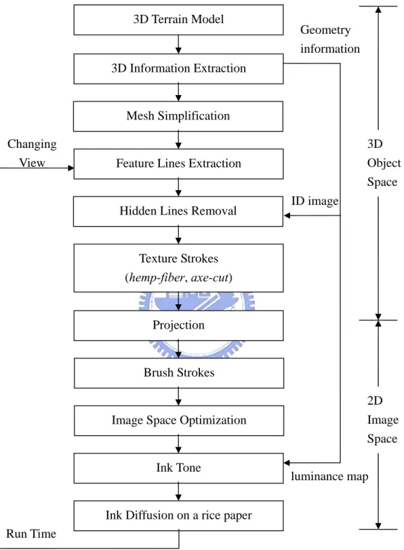
(13) 1.2 Overview In recent years, non-photorealistic rendering (NPR) approaches have received renewed interest in computer graphics-related research. Many researches addressed on Western painting, including watercolors [6, 11], impressionistic painting [21], pencil sketches [31, 32] and hatching strokes [10, 13, 20, 15, 28, 30]. These deliver good results for modeling Western painting. However, most of these methods are not fit for Chinese ink painting. Chinese ink paintings typically consist of simple strokes that convey the artists’ “deep feeling” but not just color filling or pattern placing. Simulating the style of the Chinese ink painting is not at all trivial. The style includes free brush stroke, surface wrinkle and ink diffusion on the paper [8, 22, 25].. The main goal of this thesis is to render terrain’s wrinkle automatically in Chinese landscape painting. First, a 3D terrain model is drawn with silhouette edges. Then, information on the terrain surface such as shading or orientation is used to generate texture strokes. Finally, the stylized strokes are applied to have a Chinese ink painting look. Besides the visual styles, we can navigate around the scene and show images viewed from different positions at interactive rates. Furthermore, we resolve the frame coherence problem that we can have a smoothly view while navigating. The proposed rendering technique involves many fundamental parts, as shown in Figure. 2.

(14) 1.1. The main function of each part is described as follow:. 3D Terrain Model. Geometry information. 3D Information Extraction. Mesh Simplification Changing View. 3D Object Space. Feature Lines Extraction. Hidden Lines Removal. ID image. Texture Strokes (hemp-fiber, axe-cut). Projection. Brush Strokes 2D Image Space. Image Space Optimization. Ink Tone. luminance map. Ink Diffusion on a rice paper Run Time. Figure 1.1: System architecture. 3.

(15) (1) 3D information extraction: We use OpenGL to render 3D terrain model with vertices, edges, faces and light sources. The luminance map is specified as ink tone values. The ID reference image will be used in hidden line removal step.. (2) Mesh simplification: To speedup the computation time, we reduce the total vertices of terrain model at a pre-processing step. Users can specify different levels of simplification.. (3) Feature lines extraction: This part include streamlines generation and silhouette edges detection. Streamlines are direction fields on the surface and they are computed at a pre-processing step. Silhouette edges are contour of an object that is calculated frame by frame. All these steps are done in 3D object space.. (4) Hidden lines removal: We use a fast and efficient algorithm to detect visible feature segments. Then we merge these segments into smooth and long paths for the next step.. (5) Projection: All visible feature lines are projected onto a 2D viewing plane. These projected 2D points are used as control points to apply brush strokes.. (6) Brush strokes: A physically-based brush stroke module [37] is used to simulate the Chinese style of drawing. The ink tone is specified by a luminance map.. (7) Image space optimization: We use some methods to further improve the quality of 4.

(16) synthesized images. This makes the final result the same as the traditional Chinese landscape painting.. (8) Ink diffusion: The motion of ink on the rice paper is simulated [16].. The rest of this thesis is organized as follows. In Chapter 2, we review the related works in non-photorealistic rendering. Chapter 3 describes the extraction of feature lines. In order to synthesize effects of Chinese ink painting, we introduce an applicable brush model in Chapter 4. Chapter 5 shows different kinds of rendering styles and techniques to improve the quality of synthesized images. In Chapter 6 we demonstrate results generated by our proposed system. Finally, conclusions and future work are given in Chapter 7.. 5.

(17) Chapter 2 Related Works According to different styles of painting, researches on non-photorealistic rendering [6, 11, 15, 21, 31, 32] focus on different aspects. For instance, color distribution is important while simulating oil painting, but the crucial point of Chinese ink painting is a proper brush model. Since the goal of this thesis is to simulate Chinese ink painting, we classify related researches into the following categories: silhouette algorithm, line visibility determination, stylized rendering, and brush model.. 2.1 Silhouette Algorithm Silhouettes play an important role in shape recognition because they provide one of the main cues for figure-to-ground distinction. There are so many methods handling the silhouette extracting and visibility culling problems. Saito and Takahashi [29] proposed an image-space algorithm to find silhouettes that use the z-buffer to. 6.

(18) detect edges and apply an edge detector such as the Sobel operator. Hertzmann [12] extended this method by using a normal buffer instead.. A simple object-space algorithm is based on the definition of a silhouette edge. The algorithm examines all model edges and selects only those that share exactly one front- and one back-facing polygon. Buchanan and Sousa [4] suggested using a data structure called an edge buffer to support this process for speeding up the computation time. To further speed up the brute-force algorithm, Card and Mitchell [5] suggested employing user-programmable vertex processing hardware. In this thesis, we use a simple object-space algorithm with a data structure similar to winged-edge data structure. This reduces the computation time of silhouette edges.. 2.2 Line Visibility Determination In most cases, object-space silhouette algorithms produce the problem of visibility culling. This problem is the classic computer graphics problem of hidden line removal. There are many algorithms for hidden line removal in object space. Appel [3] presented the visibility algorithm that based on the notion of quantitative invisibility (QI) – the number of front-facing polygons between the point on the edge to be rendered and the viewer. Markosian et al. [23] used a modified version of. 7.

(19) Appel’s algorithm to improve computation time. They defined the QI value as the total number of faces between a point and the viewer. Hertzmann and Zorin [13] applied this approach to their algorithm for sub-polygon silhouettes.. A simple and fast image space algorithm to determine the visibility of silhouette edges is to use the z-buffer. Silhouette edges are rendered and let the z-buffer remove the hidden lines. However, pixel accuracy and partially occluded problem are main disadvantages of z-buffer algorithm. Northup and Markosian [26] used an ID buffer to determine silhouette edge visibility. A unique color identifies each triangle and silhouette edge in this ID buffer. Isenberg et al. [18] use a similar approach. They base on their visibility test on the z-buffer instead of an additional ID buffer. In this thesis, we use ID buffer to resolve the hidden line problem because it can also identify the visible triangle surfaces that help us to determine other type of feature lines.. 2.3 Stylized Rendering There are many researches on 3D non-photorealistic rendering, such as stylized line illustrations, artistic hand-drawn illustrations, pen-and-ink drawing and hatching. Winkenbach and Salesin [38] provided a method of rendering smooth surface in pen-and-ink style. Buchanan and Sousa [31, 32] focused on physically simulating real. 8.

(20) media, including pencil, crayon, blenders and erasers. Freudenberg’s [10] method involves encoding a stroke texture as a halftone pattern. Salisbury et al. [30] introduced prioritized stroke texture whose tone value is mapped to stroke arrangement. Lake et al. [20] described an interactive hatching system with stroke coherence in the image space. Hertzmann and Zorin [13] generated high quality silhouette edges and described a scheme for placing image space strokes for cross-hatching.. Recently, many researches use principal curvature directions for surface rendering. The most natural geometric candidate is the pair of principal curvature direction fields [9, 34]. Way [36] developed a simple weighted technique by using a reference direction to generate smooth direction fields on a surface. In this thesis, we follow Way’s method to represent surface’s wrinkles because this method is suitable for generating streamlines for texture strokes of terrain’s surface.. 2.4 Brush Stroke Model For Chinese ink painting synthesis, the most important part is to have an expressive brush stroke model. Little research has addressed on simulating brush stroke and the behavior of ink. Strassmann [33] proposed a basic brush model of ink. 9.

(21) painting. He defined a 1-D array as the painting brush, and elements in the array are taken as bristles. Horace and Helena [17] proposed a method to simulate the physical process of brush stroke creation by using a 3D cone and move it dynamically. Their system focused on Chinese calligraphy.. Weng [37] introduced a 2D brush model. He defined a circle as the contact region of brush and canvas. Bristles are distributed uniformly in the contact region. While painting, the center of contact region moves along the stroke path and leads bristles moving and leaving footprints on the canvas. Various painting styles are predefined and the orientation of brush movement is taken into consideration. Strokes painted with Weng’s model looks more natural and smooth. Hence, Weng’s model is the major reference of our system because of its easy implementation and good visual effects.. Zhang [39] simulated ink behavior with Simple Cellular Automation-based simulation. They build three models: ink, brush and paper, and then take complex interaction of these models to synthesize ink strokes. Curtis [6] simulated various artistic effects of watercolor. His model is empirically-based and incorporated some physically-based models for generating watercolor strokes.. 10.

(22) Chapter 3 Feature Line Extraction This chapter describes feature lines we used to represent the Chinese landscape painting. First, 3D terrain model information is extracted. Second, the streamlines that express the wrinkles of terrain surface are constructed in a preprocess step. Third, the silhouette of the model is generated at run time. Finally, these silhouette and streamlines are projected onto a 2D viewing plane frame by frame. These 2D points are used as control points to apply the brush strokes. We will discuss how to apply brush strokes by control points in the next chapter.. 3.1 Extracting 3D Information Digital Elevation Model (DEM) is widely used in science and engineering applications. It is also known as a grid field and is a popular format of terrain files. In this thesis, we use 3DEM Visualization Software [40] to construct all of the terrain models. The grids of DEM heights were converted into adjacent triangles. The inputs. 11.

(23) of the 3D terrain polygonal models are rendered using OpenGL includes vertices, edges and faces. The lightness of shading is determined using the luminance map. The gray-scale value in the luminance map specifies the ink tone values. Geometrical information is used to detect the edges of silhouettes, generate streamlines and ridge meshes. All information can be extracted in preprocess without any user’s intervention.. 3.2 Streamline Construction To generate streamlines, we must choose some direction fields on the surface. The most natural geometric candidate is the pair of principal curvature direction fields [9, 34]. However, there are various weaknesses. For example, some fields are not defined anywhere on a sphere. Also, on flat areas when both radii of curvature are very small, the fields are likely to yield a far more complex pattern. Yutaka Ohtake et al. [27] presented adaptive smoothing tangential direction fields on a polygonal surface. Their method effectively simulated pen-and-ink drawings of 3D objects. However, Chinese landscape painting seeks to simulate the texture of a terrain’s surface. In this thesis, we follow Way’s method [36] to generate streamlines that represent the surface wrinkles of the terrain.. 12.

(24) Given a triangular surface, we first calculate the principal curvature direction at each vertex. Then, we update each vertex’s direction by calculating a weighted sum of the directions repeatedly and simultaneously. This step smoothes the direction field and preserves the coherent of the reference direction. The reference direction is the gravity direction which indicates the flow of terrain. Since DEM is a grid field of height, so given any vertex P (Px, Py, Pz), Py is the height of the vertex. Figure 3.1 r. r. shows a triangular mesh F with normal vector F n. G is the direction of gravity (0, r. r. -1, 0). G ref is the projection of vector G onto the F. The vector t(P) is the initial principal direction estimated at the vertices in the mesh, as follows:. n. t ( P) =. t ( P) + ∑ [Wi ×t (Qi )]. Wi =. i =1. n. 1 + ∑Wi i =1. ,. PQi n. ∑ PO. i. i =1. where Q are all the neighboring vertices of P and W is weighting value between PQ.. t(P1). Fn. t(P2). Gref t(P3). G. r. Figure 3.1: The reference direction G ref.. The vector t(F) is the streamline direction field combined with t(P1), t(P2), t(P3) 13.

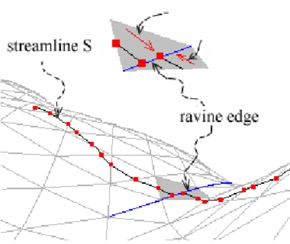
(25) r. and G ref. on. triangle F. It is defined by t(F) = αGref + (1-α)(t(P1)+t(P2)+t(P3)).. The meaning of t(F) can be explained as: if a raindrop falls on the surface F, it would flow along the streamline direction t(F). This is quite reasonable and expressible for the terrain. It also fits the features that painters used to describe the mountains.. After the streamline direction field is smoothed by the reference direction, we calculate the direction field t(F) on the face of every triangle mesh. Then, an initial point inside a triangle is selected. The streamline is traced from the point, according to Sk+1=Sk +ρt(Fk); ρ is a real number such that the line meets the edge of the triangle ; Sk+1 is located at the edge of the triangle. Streamline tracing ends when the direction conflicts with the neighboring triangles’ streamline direction, as shown in Figure 3.2, in which the streamline stops at a ravine. Using this method, each triangle mesh can generate one streamline. Figure 3.3 depicts the resulting strokes according to streamlines obtained by this method.. Figure 3.2: Streamlines construction. 14.

(26) In Chinese landscape painting, painters combine various strokes to depict terrain’s surface wrinkle. Changing the distribution of strokes, the stroke length and other factors generates different texture strokes. To further improve the quality of the final result, we add some terms that can control the distribution of streamlines while constructing streamlines. First, the density term d controls the tightness between streamlines. When we start to construct a streamline from a triangle, we first check its neighboring triangles. If more than d neighbors have constructed streamlines, the current triangle will not generate any streamline. Otherwise, it will. Second, the segment term s determines the segments of a streamline. When a streamline pass through a triangle, we call it a segment. Originally, the streamline grows until it meets the ravine edge. Now we check the total segments of a streamline at each construction step. When the total segment is greater than s, this streamline stops the construction process. Third, the angle term θ controls the slops of a streamline. When a streamline is constructed, we further check its included angle with the ground level (1, 0, 0). If the included angle is smaller than θ , this streamline is disabled. By adding this restriction, we can express the roughness of the terrain’s surface. Figure 3.3 (a) to (d) show different kinds of distribution by changing terms d, s and θ .. 15.

(27) (a) Original Streamlines. (b) Lower Density. (c) Fewer segments. (d) Greater Included Angle. Figure 3.3: Streamlines rendering.. 3.3 Silhouette Generation Since the DEM terrain data has been converted to standard triangular meshes, we need to analyze the structure of these models to determine which edges form silhouette outlines. We define a silhouette edge to be an edge that connects a front-facing triangle to a back-facing triangle. Because this condition depends both on. 16.

(28) the viewpoint and the state of the model, we should identify these silhouette edges frame by frame.. We use a brute-force approach to find the silhouette edges that simply checks every edge of the mesh. This may waste a lot of time. To speed up the silhouette identification process, we make use of a winged-edge data structure that provides local connectivity information. When checking if an edge is a silhouette edge, we find its two neighboring faces by looking up the terrain data structures. Then we only need to compare these faces’ normals with the viewing direction, we can identify if the edge is a silhouette edge. Figure 3.4 shows the silhouette edges obtained from the terrain model.. (a) Terrain Model. (b) Silhouette Edges. Figure 3.4: Silhouette generation.. 17.

(29) 3.4 Stroke Placement After we have found out streamlines and silhouette edges, the next thing we are going to do is to find out visible segments from these feature lines. Then these visible segments are merged into long paths. Finally, all the end points of the paths are used as control points to apply strokes. The following sections will describe the detailed steps.. 3.4.1 Hidden Line Removal. Once we have detected the feature lines in the current frame, the next step is to determine which portions of the silhouette edges and streamlines are visible. We make use of the “ID reference image” [19] to extract visible segments.. We create the ID reference image by first rendering the scene with each silhouette edges and each triangle mesh drawn in a color that uniquely identifies it. Then read this image from the frame buffer. Lighting and blending are disabled so that the colors are preserved exactly. Figure 3.5 shows the ID reference image of the corresponding terrain model.. 18.

(30) (a) Triangle Meshes. (b) ID reference image. Figure 3.5: ID reference image.. We next iterate over all the pixels in the reference image and build a list L of edges that contribute at least one pixel. We thus remove from consideration silhouette edges that make no contribution to the pixels of the current frame. For every streamline, we determine the visibility by checking the visibility of triangles it passes through.. Then, we scan-convert along each edge in L to determine which portions of it show up in the ID reference image, and hence are visible. We record each such visible portion, or segment. A segment consists of its two image-space endpoints and a pointer to the associate edge. To determine whether an edge e shows up in the ID reference image at a given image-space point x on e, we check the ID reference image at x, and also at nearby points (within two pixels in practice) along the image-space line perpendicular to e and passing through x. If e shows up anywhere along this line, 19.

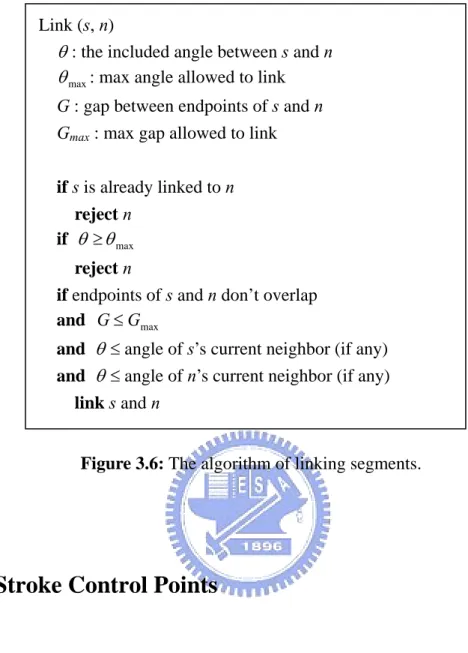
(31) we consider e to be visible at x.. 3.4.2 Artifact Removal. Since meshes do not provide perfect representation of surface and due to numerical instabilities in silhouette edges detection, we often get overlapping silhouette edges and small zig-zags in image-space. These have to be removed in order to achieve good looking results when applying styles to strokes. We resolved some well known artifacts such as triangles with two visible edges, silhouette edge clusters, silhouette stroke zig-zags, sharp angles and short segments.. 3.4.3 Linking Segments into Paths. Now we have a collection of segments that approximate the visible silhouettes of the scene. The next step is to link these segments into long paths that will form the skeleton of strokes. To do this, we first search segment’s endpoints for potential neighbors. The search is an i x i (we use i = 3) pixel local search in the ID reference image. Figure 3.6 shows the algorithm we used to compute the suitability of each potential match between segment s and neighbor n. Here we use θ max = 450 and Gmax = 5 pixels.. 20.

(32) Link (s, n) θ : the included angle between s and n θ max : max angle allowed to link G : gap between endpoints of s and n Gmax : max gap allowed to link if s is already linked to n reject n if θ ≥ θ max reject n if endpoints of s and n don’t overlap and G ≤ Gmax and θ ≤ angle of s’s current neighbor (if any) and θ ≤ angle of n’s current neighbor (if any) link s and n Figure 3.6: The algorithm of linking segments.. 3.4.4 Stroke Control Points. After long silhouette paths and streamlines are extracted, we then apply stroke along these paths. Our brush model is constructed using the precise and flexible Cardinal spline. Cardinal spline is an interpolated but not approximated curve, which passes through all the specified control points. So we use endpoints of silhouette paths and streamlines as control points. The other advantage of Cardinal spline is its flexibility. The terrain can be painted softer or harder. Cardinal spline enables slackness control by changing parameter t. A small t implies a slacker curve. Figure. 21.

(33) 3.7 displays the precision and flexibility of the Cardinal spline. Once the control points are determined, then we can apply the Chinese style of strokes. We will discuss how to achieve this in the next chapter.. (a) t = 0.2. (b) t = -0.5 Figure 3.7: Cardinal curve with different t.. 3.5 Mesh Simplification The Chinese landscape painting pays attention to express an artistic concept. So painters usually care about an overall arrangement among objects. The detail of an object is not so important; we only need to depict major characteristics. To further improve the quality and performance of the rendered image, we have some ideas for synthesizing Chinese landscape painting. Since we don’t need “detail” information of a model, why don’t we simplify the triangle meshes? By doing this, performance can be increased and feature lines extracted from the simplified model can be relative meaningful. We use Progressive Mesh approach [14] to reduce the terrain model. We can change the accuracy of the model by adjusting the total number of vertices in the model. Figure 3.8 shows different levels of simplification. 22.

(34) (a) Original Meshes. (b) 75% of vertices. (a) 50% of vertices. (b) 25% of vertices. Figure 3.8: Progressive mesh.. 23.

(35) Chapter 4 Painting Algorithm In this chapter, we describe the painting algorithm we used to simulate Chinese ink painting styles. After we generate feature lines, brush strokes should be applied on them. There are many well established painting algorithms and brush models. Some of them are physically-based and some are parameter-based model. For example, Weng’s brush model [37] is dedicated to Chinese ink painting and Curtis’s model [6] simulated various effects of watercolor.. There are three main components in our painting algorithm. First, a physically based brush model describes the shape of the brush, the number and locations of bristles. Second, a brush movement control mechanism determines the position and orientation of a brush during the painting process. Third, an ink depositing mechanism simulates various brush stroke effects such as gradient effect, dry brush effect, concentration of ink and the difference among bristles.. 24.

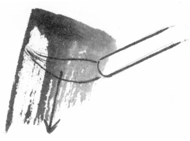
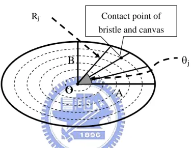
(36) While painting, our brush model will move along the path of stroke and deposit ink on the canvas. In Section 4.1 we introduce a deformable brush model. Section 4.2 discusses the movement, pressure variation and rotation of brushes. Then the ink depositing model is presented in Section 4.3. The ink depositing model controls the amount of ink that deposited by each bristle at each time instant thus generates various effects of brush strokes.. 4.1 Brush Model Horace and Helena [17] used a 3D model to simulate the brush, and used an ellipse to simulate the contact region of the canvas and brush. Horace’s model is usually applied on calligraphy because it performs turning effects very well. Weng’s model [37] distributes bristles uniformly in a 2D circle. In Chinese ink painting, since turning effects are not so emphasized, a 2D brush model is enough to simulate painting strokes.. Weng’s model focused on simulating center-stroke effect. However, in Chinese landscape painting, side-stroke effect is also necessary. Especially when we simulate axe-cut Ts’Un painting styles, almost every stroke is side-stroke. Unlike centerstroke’s brushwork, side-stroke tilts the brush while painting. Chiang [7] modified. 25.

(37) Weng’s model to achieve side-stroke effect. The contact region of side-stroke is similar to an ellipse, and the tip of the brush is on the side, as shown in Figure 4.1.. Figure 4.1: Side-stroke effect.. To implement both center-stroke and side-stroke effects, we use a deformable ellipse structure to simulate the contact region of the canvas and brush. By adjusting the ratio of ellipse’s main shaft and countershaft, we can simulate various side-stroke styles. When the shaft ratio is equal to one, the contact region is a circle and center-stroke effect is simulated. As shown in Figure 4.2, the distribution of bristles is similar to concentric ellipses. O is the center point of concentric ellipses. We use the outmost ellipse (E1) as the criterion and distribute other ellipses inside E1 in a ratio of equality. We define the Y direction of E1 as the main shaft (B). B is also the standard of the shaft length. The X direction of E1 is the countershaft (A). The shaft length of each ellipse is defined as follows:. 26.

(38) ai = A ×. i i , bi = B × I I. where ai and bi is the main shaft and the countershaft of the ellipse Ei. I is the total number of ellipses and i is the index of ith ellipse.. E1. x2 y2 Ei： a 2 + b2 = 1 i i. Y. B X O. A. ( brush moving direction). Figure 4.2: The contact region of brush.. The parametric equation of each ellipse Ei is:. xi = ai cos u yi = bi cos u. u ∈ [0,2π ]. Inside the contact region, contact points of each bristle and canvas can be figured by calculating the intersection points of concentric ellipse and lines radiated from center point O. In Figure 4.3, each radiant line segment divides the ellipse into regions. 27.

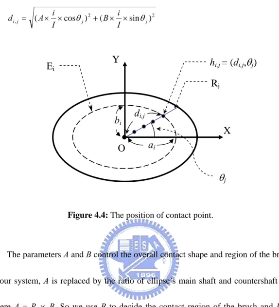
(39) Rj in a equal angle. The angle between radiant line and A can be calculated by. θ j = 2π ×. j J. where θj is the included angle between A and Ohi , j . J is the total number of divisions and j is the index of jth division.. Contact point of bristle and canvas. Rj. θj. B O. A. Figure 4.3: The contact point of each bristle.. So, the contact point of each bristle is the intersection point of Rj and Ei. Figure 4.4 shows the contact point of bristle hi,j. We use the polar coordinate to represent the position of hi,j. The center point of the polar coordinate is O.. hi,j = (di,j,θj). where i is the index of the ellipse and j is the index of the division. di,j is the distance from hi,j to O. di,j can be calculated by:. 28.

(40) i i d i , j = ( A × × cosθ j ) 2 + ( B × × sin θ j ) 2 I I. Ei. hi,j = (di,j,θj). Y. Rj bi. di,j X ai. O. θj. Figure 4.4: The position of contact point.. The parameters A and B control the overall contact shape and region of the brush. In our system, A is replaced by the ratio of ellipse’s main shaft and countershaft (R) where A = R × B. So we use B to decide the contact region of the brush and R to determine the shape. I controls the number of concentric ellipses and J decides the number of contact region divisions. Both I and J are related to the distribution density of bristles. Since we have parameterized the contact points of the bristles, we can generate the desired brush styles by adjusting B, R, I and J. Both center-stroke and side-stroke effect can be simulated by this method.. 29.

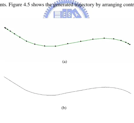
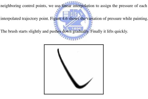
(41) 4.2 Brush Movement Control Mechanism During painting process, the brush moves its contact region along the stroke trajectory and deposits ink to generate expected strokes. In this Section, we discuss three parameters that varied constantly during this process: position of the contact region, size of the contact region and brush orientation.. We use Cardinal Spline to simulate the stroke trajectory. Since it is an interpolating curve, we could obtain interpolated points between two neighboring control points. Figure 4.5 shows the generated trajectory by arranging control points.. (a). (b). Figure 4.5: (a) Control points (b) Interpolating curve.. While painting, the center of contact region goes through these interpolated points orderly and lead surrounding bristles leaving footprints on the canvas. Assume 30.

(42) the center of contact region on the canvas is (ox, oy), the position of bristle hi,j can be calculated as below:. '. hi , j , x = hi , j , x + O x = ( A × '. hi , j , y = hi , j , y + O y = ( B ×. i × cos θ j ) + O x I i × sin θ j ) + O y I. While painting, the pressure of the brush affects the size of the contact region. It also affects the amount of ink deposition and we will discuss this in the next section. To ensure the brush pressure changes naturally and smoothly between two neighboring control points, we use linear interpolation to assign the pressure of each interpolated trajectory point. Figure 4.6 shows the variation of pressure while painting. The brush starts slightly and pushes down gradually. Finally it lifts quickly.. Figure 4.6: Linear variation of brush pressure.. Assume we have n + 1 control points c1, c2, c3, …, cn, cn+1, we can separate this curve into n segments s1, s2, s3, …, sn. When an interpolated trajectory point d is inside 31.

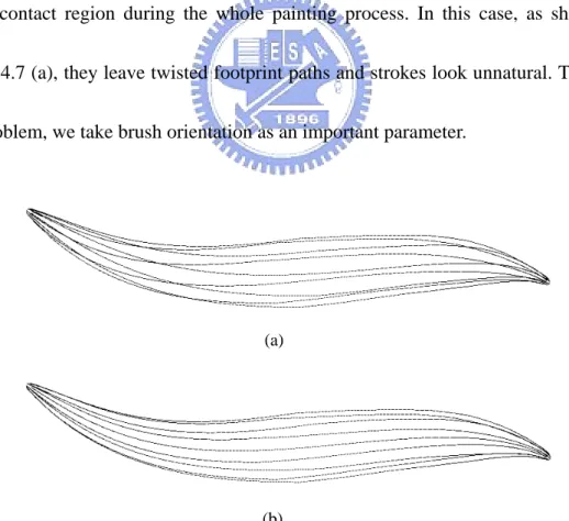
(43) segment si, we use the following equation to get d’s pressure value:. p d − pc i pci +1 − pci. =. where 0≦ pci 、. u d − uc i uci +1 − uci. pci+1 ≦1 is the pressure value of ci and ci+1 respectively. 0≦ uci 、. u ci +1 ≦1 is the Cardinal Spline parameter of ci and ci+1 respectively.. When the brush moves along the stroke trajectory, it’s orientation is changed constantly. If the brush orientation is never changed, bristles stand in fixed positions in the contact region during the whole painting process. In this case, as shown in Figure 4.7 (a), they leave twisted footprint paths and strokes look unnatural. To solve this problem, we take brush orientation as an important parameter.. (a). (b). Figure 4.7: (a) Fixed orientation (b) Orientation by tangent vector.. 32.

(44) In Figure 4.7 (b), when the brush moves along a track and comes to kth trajectory point (dk), the moving orientation is determined by the tangent of dk. We approximate it by:. T ( xk , y k ) =. yk − yk −1 xk − xk −1. φ k = tan −1 (T ( x k , y k )). where T(xk, yk) is the tangent of dk on the curve.. Ellipse axis A (Align to Tk). dk(xk, yk) Tk. hi , j. X dk-1(xk-1, yk-1). hi', j Figure 4.8: Brush orientation according to tangent vector Tk.. Figure 4.8 shows the bristle position before and after the orientation. Bristles in a contact region rotate θ with respect to the center of contact region. The equation we obtain new coordinates of bristles is as follow: 33.

(45) hi , j , x = ( A ×. i i × cos θ j × cos θ − B × × sin θ j × sin θ ) + O x I I. hi , j , y = ( A ×. i i × cos θ j × sin θ + B × × sin θ j × cos θ ) + O y I I. where θ is the difference of angles between dk and dk-1.. 4.3 Ink Depositing Mechanism Weng’s model [37] has 4 parameters to control painting styles: decreasing, concentration, difference and discontinuity. These parameters satisfy the request of simulating calligraphy or plant in Chinese ink painting. However, to present rock texture in Chinese landscape painting, we need more parameters to depict effects of dry stroke. In Weng’s model, ink quantity and ink color are equivalent, so it is hard to simulate strokes with dark ink color but low ink quantity. To solve this problem, we use two parameters to present ink quantity and ink color respectively. In Section 4.3.1, we explain how to modify Weng’s ink decreasing effect to achieve dry strokes. We introduce basic painting styles inherited from Weng’s model in Section 4.3.2. Finally, pressure mechanism for center-stroke and side-stroke is described in Section 4.3.3.. 4.3.1 The Ink Decreasing Effect. As shown in Figure 4.9, we can see that color drawn by the brush is decided by. 34.

(46) the mixed rate of water and ink. If the brush is total soaked in water and then ink is soaked on the tip of the brush, ink and water will blend gradually. So the color of the painted stroke will change from dark to light. To simulate this kind of effect, we apply additional parameters to control the ink color. We set each stroke’s beginning and ending ink color. Then we use linear interpolation to get the ink decreasing effect, as shown in Figure 4.10.. (a). (b). (c). (d). Figure 4.9: (a) Soaked in water (b) Soaked with ink (c) Blending (d) Decreasing.. Figure 4.10: The ink decreasing effect.. 35.

(47) 4.3.2 The Characteristic of Ink. Our brush model inherits basic painting styles of Weng’s model which are introduced briefly as follows:. 1. The Ink Soaking Variation. In a brush stroke, the concentration of ink is not uniform. This could be caused by ink itself or made by painters. Some effects, such as the leaves of bamboo, are depicted with different concentration of ink. Weng’s model proposed 4 different concentration types, in which ink concentration is linearly interpolated in the contact region, to simulate different aroma, as shown in Figure 4.11.. Figure 4.11: A stroke with soaking variation.. 2. The Bristle Fan-Out Effect. To simulate this effect, as shown in Figure 4.12, a random array, difference, is proposed. Values in difference are ranged from -5 to 5. When we construct a brush, each bristle is mapped to an element of difference to get its difference value, which. 36.

(48) will be added to ink concentration in the bristles to make the ink color darker or lighter.. Figure 4.12: A stroke with ink fan-out.. 3. The Bristle Dry-Out Effect. The bristle dry-out effect occurs when deposited ink is less (lighter) than a threshold. To simulate this effect, as shown in Figure 4.13, the max gap size is predefined in an array, discontinuity, and each bristle is mapped to discontinuity randomly to get its max gap size. Once a bristle deposits ink discontinuity, its discontinuous gap size can not be larger than its max gap size. Besides, the discontinuous gap size keeps decreasing until it is equal to zero during the brush moving process.. Figure 4.13: A stroke with ink dry-out.. 37.

(49) 4.3.3 The Pressure Mechanism. For a single brush, the size of the contact region is different if we apply different pressures. On the other hand, the deposited ink from the brush depends on not only the remnant quantity of the ink but also the pressure of the brush. So it is important to discuss relations of deposited ink and pressure. However, the way to put brush to canvas is different between center-stroke and side-stroke, so we propose the pressure mechanism for both cases.. 1.. Center-Stroke. The brush of center-stroke goes straight down and the pressure of the brush influences the size of the contact region and the quantity of deposited ink. In Figure 4.14, the gray area means the region that the brush contacts with the canvas. The deep or light color of the ink shows the weighting value Wp of deposited ink for each bristle. Compare to case (a) and case (b) in Figure 4.14, the pressure of (b) is greater than (a), so the size of the contact region is larger and the quantity of the deposited ink is also larger. We define Wp as:. ⎧ ⎪no touch ⎪ Wp = ⎨ ⎪ ((1 - d i, j ) × p + p)/2 ⎪ d I, j ⎩. ,. d i, j d I, j. ,. d i, j d I, j. >p ≤p. 38.

(50) where di,j is the distance from hi,j to the center of ellipse O and dI,j is the distance from hI,j to O. 0≦p≦1 is the pressure of the brush. We also know that:. di,j = dI,j ×. i I. So, Wp can be reduced to:. ⎧ ⎪⎪no touch Wp = ⎨ ⎪ ((1 - i ) × p + p)/2 I ⎩⎪. i , >p I i , ≤p I. Figure 4.14: The relation of pressure, contact region and depositing ink.. We use Weng’s model to calculate the ink value of bristle hi,j, then we multiply it by Wp that we can simulate stroke with pressure variation. Figure 4.15 shows the pressure P increases from 0 to 1 and then decreases from 1 to 0. It simulates the stroke when a painter is drawing. The painter presses down the brush gradually. Then he pushes down entirely when it comes to a turning point. Finally, he lifts the brush by degree. Case (a) and case (b) shows the results of different brush size. 39.

(51) (a). (b). Figure 4.15: Strokes with pressure variation. P changes from 0 ->1 ->0. (a) B = 40, R = 1, I = 80, J = 30. (b) B = 10, R = 1, I = 20, J = 5.. 2.. Side-Stroke. The side-stroke tilts the brush while painting, just like Figure 4.1 in Section 4.1. When the brush lifts up, the size of the contact region gets smaller from a single side to the center of the brush. In Figure 4.16, the brush pressure of (a) is smaller than (b), so the contact region is smaller. The weighting value Wp of each bristle for side-stroke is defined as follows:. 40.

(52) ⎧ ⎪⎪no touch Wp = ⎨ ⎪P ⎪⎩. , ,. h i, j,y + B 2B h i, j,y + B 2B. >p ≤p. where hi,j,y is the y-coordinate value of hi,j.. Moving Direction. Figure 4.16: Side-stroke lifts up the brush from a single side.. Figure 4.17 is the results of side-stroke synthesis. The brush model moves from up to down and the shape of the stroke shrink from left side to center. (a) and (b) shows two kinds of pressure variation. This simulates different styles of side-stroke brushes.. 41.

(53) (a). (b). Figure 4.17: Different pressure variation of side-stroke. (a) Small axe-cut Ts’Un, R = 0.2. (b) Big axe-cut Ts’Un, R = 0.3.. 42.

(54) Chapter 5 Landscape Painting Styles Chinese ink painting has a long history over three thousand years. It heavily stresses the notion of “implicit meanings” by abstracting objects. In the Tang dynasty (618 – 907 AD), the range of subjects in paintings expanded and landscape became as a distinct category. Chinese landscape painting provided a more spontaneous style that captured images in abbreviated suggestive forms. Chinese landscape painting has been cultivated by masters through a long evolution, into an exquisite art form.. In Chinese landscape painting, rocks are primary objects because of the power to create the mood. Artists use the Chinese character Ts’Un, also meaning wrinkles, to represent texture strokes when applied to rock formations. Over the centuries, masters of Chinese landscape painting developed various Ts’Un techniques. Among these Ts’Un styles, hemp-fiber strokes and axe-cut strokes are two major types of Ts’Un techniques.. In previous chapters, we show how to extract feature lines and establish 43.

(55) appropriate brush models. Theoretically, we have successfully synthesized Chinese style images by applying strokes on those feature lines. However, these results are quite different from painters’ works. We can’t capture characteristics of Ts’Un styles by a simple mapping from a stroke to a feature line. Hence, we design some experimental based methods to improve the quality of synthesized images. All these procedures are done in image-space. In Section 5.1, we give an introduction to. hemp-fiber Ts’Un. Axe-cut Ts’Un is described in Section 5.2. Section 5.3 describes image-space optimization methods we used to improve the quality of results. Section 5.4 shows the frame coherence of each painting style.. 5.1 Introduction to Hemp-Fiber Ts’Un Hemp-fiber strokes, spreads and weaves like the fibers of the hemp from which it takes its name. This may be the most important stroke in Chinese landscape painting. Several texture strokes have been developed from the hemp-fiber strokes. Long. hemp-fiber strokes express relatively smooth surfaces, while short hemp-fiber strokes indicate a more wrinkle surface. The short hemp-fiber Ts’Un is developed by the great Southern School master Tung Yuan (907 – 960 AD), which was varied and generally favored by the literati painters, who dominated mainstream Chinese landscape painting, beginning with the emergence of the Four Masters of the Yuan dynasty 44.

(56) (1279 – 1368 AD). The most important of the Four Masters, Huang Gung-Wang (1269 – 1354 AD), practiced the strokes in a loose, calligraphic fashion, as show in Figure 5.1.. Figure 5.1: Hemp-fiber Ts’Un by Huang Gung-Wang.. 5.2 Introduction to Axe-Cut Ts’Un The axe-cut stroke is a slanted stroke used in painting in much the same way as an axe is used to cut wood. It is excellent for depicting smooth cliffs and flat, planar surfaces of rock. The stroke also effectively describes angularly shaped rocks of crystalline quality and sedimentary rocks displaying layered structures. The axe-cut Ts’Un was developed earlier during the Sung dynasty (960 – 1279 AD) by Li-Tang. 45.

(57) (1049 – 1130 AD). This stroke dominated Southern Sung landscape painting between the 12th and 13th centuries. The best-known exponents of the axe-cut Ts’Un are Ma Yuan and Hsia Kwei, associated with the Northern School of landscape painting, which thrived, in particular, during the Sung dynasty. Figure 5.2 is the axe-cut Ts’Un drawn by Hsia Kwei.. Figure 5.2: Axe-cut Ts’Un by Hsia Kwei.. 5.3 Image Space Optimization In this section, we describe how to make the computer-generated images visually similar to painters’ works. According to our observation, we conclude some 46.

(58) characteristics for hemp-fiber Ts’Un and axe-cut Ts’Un. So we design methods to make each applied brush stroke with a suitable style. Since our brush model is controlled by specific parameters, so we can change strokes’ appearances by tuning each parameter. All these steps are done in image-space.. 5.3.1 Stroke Length Control. When applying strokes, the position, shape and length are decided by control points. All these control points are extracted from object space, as described in Chapter 3. So, at each frame, after we project these 3D points to image-space, we can not guarantee the distance between control points. Some control points are close together while others are distant. Besides, the total length of a brush stroke is also uncontrollable. Some strokes look too long, and some are too short. These situations make us difficult to tune up the rendering style of each stroke. Therefore, we propose a mechanism to adjust distances between control points and strokes’ length. If the distance between two control points is far away, we insert additional control points. Otherwise we discard unnecessary control points. If the total length of a stroke is too long, we divide the stroke into several strokes. If the length is too short, we abandon this stroke. The algorithm is shown in Figure 5.3.. 47.

(59) Dmax: max distance allowed between two neighboring control points Dmin: min distance allowed between two neighboring control points Lmax: max length allowed for a stroke Lmin: min length allowed for a stroke L: total length of current stroke s for every control points ci in s D: distance between ci and ci+1 if( D > Dmax) insert new control point(s) between ci and ci+1 if( D < Dmin) remove ci+1. L=L+D if( L > Lmax) terminate this stroke and start a new stroke move to next control point end of for loop if(L < Lmin) reject current stroke. Figure 5.3: The algorithm of stroke length control.. 5.3.2 Layered Strokes. In Chinese landscape painting, artists use the variation of ink color to represent the light and shade. In the brightness area, lighter color is used and few strokes are drawn. In the shaded area, painters use dark ink color and draw more strokes. Besides, In a brightness area or a shaded area, we can still tell different tones of ink. To reach this kind of effect, we bring up the idea of layered strokes. We classify all strokes into 48.

(60) three kinds of layers. One is the darkest layer, the other is the middle layer, and another is the brightest layer. Each layer stands for a degree of ink tone. When all strokes are drawn on layers and each stroke’s ink value is according to luminance map, the synthesized image shows light and shade. The result is more natural and similar to artists’ works. Figure 5.4 (a) is the result before the layer conception, and (b) is the result after applying layered strokes.. (a). (b). Figure 5.4: (a) Without (b) With layered strokes.. To preserve frame coherence, the layer ID for each stroke should be fixed. To solve this problem, we define not only layer ID but also some stroke parameters after streamlines are constructed (as described in Section 3.2). Parameters, such as the size of the brush, the number of bristles, the decreasing rate of ink and water, and so on, affect the style of each stroke. The variation of each stroke also makes the result more realistic to artists’ creations. Since streamlines are consistent, layer ID and stroke 49.

(61) parameters are fixed, when the view point is moving, we can preserve the frame coherence.. 5.3.3 Mechanism for Hemp-Fiber Ts’Un. In this section, we propose two mechanisms to improve the quality of computer generated hemp-fiber Ts’Un. The first mechanism is horizontal perturbation. When artists’ draw the hemp-fiber stroke, they wiggle the brush and the stroke looks like the hemp. So, we also want to wiggle the applied strokes. Instead of wiggling the strokes, we perturb control points in the direction perpendicular to the brush moving direction. The scale of the perturbation level depends on the length of the stroke multiplied by a sin wave. As shown in Figure 5.5 (b), strokes are perturbed while (a) are not. We use following equations to achieve the wiggle effect.. v C ′( x, y ) = C ( x, y ) + (ρ × L × sin( f ) × D ). where C ′( x, y ) is the perturbed location of control point C. C ( x, y ) is the original location of control point C. ρ is weighting value. L is the length of the stroke. f is v the frequency of the sin wave and D is the direction perpendicular to the brush moving direction.. 50.

(62) (a). (b). Figure 5.5: (a) Without (b) With horizontal perturbation.. The second mechanism is reverse drawing of strokes. We observe that in hand-drawn creations, artists draws stroke densely and tightly at the bottom of the rocks. The reason artists want to emphasize the shadow part of the terrain. Usually, the shaded area lies at the lower part of rocks where the light is occluded. Therefore, we also want to express this kind of effect. Since the construction of streamlines is from top to down, we draw the strokes in reverse direction. We apply strokes from bottom to top. More strokes are drawn at the bottom of rocks and peaks of the mountains are drawn with sparse strokes. Figure 5.6 is the comparison before and after reverse drawing of strokes.. 51.

(63) (a). (b). Figure 5.6: (a) Without (b) With reverse drawing of strokes.. 5.3.4 Mechanism for Axe-Cut Ts’Un For axe-cut Ts’Un, we apply center-strokes on visible silhouette edges and draw side-strokes along streamlines. This results in an impressive grand sight. In some cases, the terrain is not so cliffy but we still want to express it in axe-cut style. In this kind of situation, we notice if we use the same process as an erect and flat rock does, the synthesized result looks unnatural. Painters draw this kind of rocks with a slope. Each stroke is tilted with a small amount of angle from the original streamline direction. To realize this effect, we find a direction intersected with the streamline direction with a specific included angle θ , then we apply the stroke along this direction. We constantly apply strokes along the streamline until it meets the terminal point. In Figure 5.7, (a) is the original axe-cut strokes and (b) is the results with tilt strokes. 52.

(64) (a). (b). stroke direction. stroke direction. streamline direction. streamline direction (c). Figure 5.7: (a) Without (b) With (c) Sketch (of) tilt strokes.. 5.4 Frame Coherence Frame coherence is an open issue in NPR related researches. If the placement and style of strokes are quite different between two consecutive frames, it will cause the un-coherent problem. In this thesis, we apply strokes on silhouette edges and streamlines. Since streamlines are constructed in a preprocess step, the position of. 53.

(65) each streamline is fixed. Furthermore, we preserve stroke parameters such as the size of the brush, the number of bristles, the decreasing rate of ink, water, and so on. When strokes are applied at each frame, we guarantee that each stroke is located at the same position and has same stroke parameters. Figure 5-8 shows the coherence between frames and the painting style is hemp-fiber Ts’Un. Figure 5-9 is the coherence of. axe-cut Ts’Un.. Figure 5.8: Frame coherence of hemp-fiber Ts’Un.. 54.

(66) Figure 5.9: Frame coherence of axe-cut Ts’Un.. 55.

(67) Chapter 6 Results In this chapter, the implementation and results are presented. Our system is implemented in C++ language on PC with P4 1.8GHz CPU and 512 MB RAM.. Figure 6.1 is the system flow chart. The input is a 3D terrain model and then streamlines are constructed. Silhouettes and ID reference images are calculated frame by frame. Finally, different styles of brush strokes are applied to synthesize the final results. Figure 6.2 and 6.3 are Chinese landscape painting results of hemp-fiber Ts’Un, and Figure 6.4 and 6.5 are results of axe-cut Ts’Un. The upper image of each Figure is the original 3D model and the lower image is the synthesized result. In Figure 6.3, the 3D model imitates the scene of Lan-Yan River and Central Range in Taiwan. In Figure 6.5, the model simulates the Grand Canyon in the United States.. 56.

(68) Table 6.1 is the performance measurements of our system and the comparison between Way’s method [36]. The resolution of the image size is 800 x 600. The first column refers to the Figures. The second column is the polygons of the 3D terrain model and the third column is the number of vertices. The fourth column indicates the painting styles. The fifth and sixth columns display the computation time of .Way’s and our method. We improve the computation time at about 50 times than Way’s method.. # polygons. # vertices. Styles. Way’s method. Our method. (sec / fps). (sec / fps). Fig. 6.2. 1,196. 600. hemp-fiber. 7.415 / 0.13. 0.126 / 7.93. Fig. 6.3. 5,614. 2,809. hemp-fiber. 11.203 / 0.09. 0.192 / 5.21. Fig. 6.4. 3,694. 1,849. axe-cut. 8.027 / 0.12. 0.165 / 6.05. Fig. 6.5. 6,948. 3,476. axe-cut. 10.018 / 0.10. 0.183 / 5.46. Table 6.1: Performance measurements.. 57.

(69) (a) 3D terrain model. (b) Wireframes. (c) ID reference image. (d) Silhouette edges. (e) Streamlines. (f) Silhouette strokes. (g) Silhouette and streamline strokes with hemp-fiber Ts’Un. Figure 6.1: System flow chart. 58.

(70) Figure 6.2: Hemp-fiber Ts’Un.. 59.

(71) Figure 6.3: Lan-Yan river with hemp-fiber Ts’Un.. 60.

(72) Figure 6.4: Axe-cut Ts’Un.. 61.

(73) Figure 6.5: Grand canyon with axe-cut Ts’Un.. 62.

(74) Chapter 7 Conclusions and Future Works In this thesis, we propose an interactive navigation system in Chinese ink painting styles. A specific 3D terrain model is drawn automatically with silhouettes and texture strokes that represent the wrinkles of surfaces. We implement two major texture strokes for terrain’s surface using traditional brush techniques in Chinese landscape painting. Besides, users can navigate around the scene with different viewing directions with frame coherence. The proposed rendering technique involves several fundamental parts: 3D information extraction; control lines construction; projection on 2D image; applying brush stroke and ink diffusion. The results of this thesis can be applied to computer games or virtual reality applications.. However, there are still some issues left to be studied in the future. (1) This thesis focuses on two main texture strokes. Although hemp-fiber Ts’Un and. axe-cut Ts’Un are the major texture strokes in Chinese landscape painting, many others should be developed. Developing other strokes would not be too difficult. 63.

(75) since the concept of texture is very similar to these two strokes. (2) A few recent studies have addressed real-time rendering. So far, the framework for graphics hardware is fit for photo realistic rendering. How to use hardware capability to resolve time consuming jobs of NPR, such as physically-based brush model and ink diffusion simulation will be a challenge work in the future. (3) Normally, there are many objects in Chinese landscape painting, such as trees, river, lake, fall, cloud, ship and house…etc. Integrating with these objects is an interesting and important work.. 64.

(76) Reference. [1] 王耀庭編，「山水畫法 1、2、3」，雄獅圖書公司，民國七十三年三月。 [2] 鄭明編著，「中國山水畫技法」，藝風堂出版社，民國七十六年三月出版。 [3] A. Appel, “The Notion of Quantitative Invisibility and the Machine Rendering of Solids,” Proc. ACM National Conf., Thompson Books, pp. 387-393, 1967. [4] J.W. Buchanan and M.C. Sousa, “The Edge Buffer: A Data Structure for Easy Silhouette Rendering,” Proc.1st Int’l Symp. Non-Photorealistic Animation and. Rendering, ACM Press, pp. 39-42, 2000. [5] D. Card and J.L. Mitchell, “Non-Photorealistic Rendering with Pixel and Vertex Shaders,” Vertex and Pixel Shaders Tips and Tricks, W. Engel, ed., Wordware, 2002. [6] J. Curtis Cassidy, D. Anderson Sean, E. Seims Joshua, W. Fleischer Kurt, H. Salesin David, “Computer-Generated Watercolor,” Proc. of SIGGRAPH’97, pp. 421-430, 1997. [7] Chun-Sung Chiang, “The Synthesis of Rock Textures in Three-Dimensional Chinese Landscape Painting,” Ms thesis, National Chiao Tung University, October 2001. [8] Chow Chian Chiu and Chow Leung Chen Ying, “Chinese Painting: A Comprehensive Guide,” Published in 1979 by Art Book Co., Ltd. [9] G. Elberg, “Interactive line art rendering of freeform surfaces,” Computer. Graphics Forum, Vol. 18, No. 3, pp. 1–12, 1999. [10] B. Freudenberg, “Real-Time Stroke Textures,” (Technical Sketch) SIGGRAPH 65.