一個照相手機上的牛眼碼解碼系統

國

立

交

通

大

學

多媒體工程研究所

碩

士

論

文

一 個 照 相 手 機 上 的 牛 眼 碼 解 碼 系 統

A Decoding System of MaxiCode using the Camera

Mobile Phone

研 究 生：郭益成

指導教授：陳玲慧 教授

一個照相手機上的牛眼碼解碼系統

研究生：郭益成 指導教授：陳玲慧 博士

國立交通大學多媒體工程研究所

摘要

在本論文中，我們提出了一個牛眼碼(MaxiCode)的解碼系統，並

實作於照相手機上。牛眼碼是一種尺寸固定的矩陣式二維條碼，主要

為運輸業所使用來儲存貨物運送資訊。論文中，我們利用照相手機對

牛眼碼取像，再對拍下的影像作處理。首先，我們利用邊緣點的資訊，

對影像進行二值化的處理。對二值化後的影像，利用細線化處理後的

結果，尋找最大的連通分量(Connected Components)，以定位牛眼碼

的探測圖案(Finder Pattern)。對於牛眼碼在圖片中可能旋轉的情形，

利用定位圖案(Orientation Patterns)將條碼轉正。而拍照所造成條碼邊

界的形變，利用反透視轉換(Inverse Perspective Transformation)來校

正。最後以水平投影的方式擷取出資料點的長度，轉換成對應的模組

來進行解碼的動作。實驗結果顯示本系統能正確且有效率的對牛眼碼

圖片進行解碼。

A Decoding System of MaxiCode using the Camera Mobile

Phone

Student: Yi-Cheng Kuo Advisor: Dr. Ling-Hwei Chen

Institute of Multimedia Engineering

National Chiao Tung University

Abstract

In this thesis, we construct a MaxiCode decoding system, and we implement it on the camera mobile phone. MaxiCode is a fixed-size matrix 2D barcode, and it is often used by transportation industry to record the transportation information of packages. In our system, we process the MaxiCode’s picture which is taken by the camera phone. Firstly, the edge points of the picture are used for the image binarization. Next, we use the thinned connected components to locate the Finder Pattern of MaxiCode, and we find the Orientation Pattern of Maxicode to rotate the code into the right position. Then we extract the boarders of MaxiCode, and we use inverse perspective transformation to rectify the code shape. Finally, the run-length of data points are extracted by horizontal projection, and the modules corresponding to the run-length are taken to decode. Experimental results show that the system can decode the MaxiCode image correctly and efficiently.

ACKNOWLEDGMENTS

這篇論文的完成，首先要感謝指導教授陳玲慧博士，在這兩年碩

士生涯中，在課業上和生活上給予的指導和關心，讓我在交大學到的

不僅是學業上的知識，還有更多做人做事的道理。此外，感謝葉俊才

學長與趙怡晴學姊額外給予的指導，使整篇論文更趨完善。

接著，要謝謝實驗室一起生活一起奮鬥的夥伴們，博士班的學長

姐們，萓聖、民全、文超、惠龍、俊旻、占和、盈如以及芳如，大我

們一屆的學長姐偉全、子翔、信嘉及薰瑩，以及同屆的同學，明旭、

志鴻和志達和學妹佳瑄，因為有大家的陪伴，讓我兩年的碩士生涯過

得充實又豐富；另外還有大學時期的同窗好友，陪我一同玩樂也一同

為論文而奮鬥，為我的碩士生涯增添許多色彩。

最後要感謝我的父母，給了我相當好的環境能夠專心於研究上，

讓我無後顧之憂。謹以此篇論文獻給我的父母，以及所有關心我、鼓

勵我的人。

TABLE OF CONTENTS

ABSTRACT (IN CHINESE)...i

ABSTRACT (IN ENGLISH) ...ii

ACKNOWLEDGMENTS (IN CHINESE) ... iii

TABLE OF CONTENTS...iv

LIST OF FIGURES ...vi

LIST OF TABLES... viii

CHAPTER 1 INTRODUCTION ...1

1.1 Motivation...1

1.2 MaxiCode...1

1.3 Related Work...3

1.4 Organization of the Thesis ...4

CHAPTER 2 PROPOSED METHOD...5

2.1 Symbol Description of MaxiCode ...6

2.1.1 Single Module...6 2.1.2 Row of Module ...6 2.1.3 Finder Pattern...7 2.1.4 Orientation Pattern...8 2.1.5 Quiet Zone ...9 2.2 Image Binarization...10

2.2.1 Edge point extraction ...11

2.2.2 Minimum mean square error...13

2.3 Finder Pattern Location...15

2.4 Orientation Correction ...17

2.4.1 Counting single module length ...18

2.4.2 Locating Orientation Patterns ...19

2.4.2.1 Orientation pattern runs analysis ...20

2.5 Code Shape Rectification...25

2.5.1 Boarder Extraction ...26

2.5.1.1 Quiet Zone Detection...26

2.5.1.2 Swing to find boarder...27

2.5.2 Inverse Perspective Transformation...28

2.6 Data Extraction ...30

2.6.1 Module run length counting...30

3.1 Controlled Environment...32

3.1.1 Rotation...33

3.1.2 Different Lighting Sources ...35

3.1.3 Oblique...36

3.1.4 Different Focal Distance ...39

3.2 Uncontrolled Environment...40

CHAPTER 4 CONCLUSION...44

LIST OF FIGURES

Fig. 1.1 An example of MaxiCode...2

Fig. 2.1 Flow diagram of the decoding system...6

Fig. 2.2 An example of a single module. ...6

Fig. 2.3 An example of odd rows and even rows...7

Fig. 2.4 An example of adjacent black modules. ...7

Fig. 2.5 An example of the finder pattern relative to the adjacent modules. ...8

Fig. 2.6 The orientation patterns relative to the finder pattern. ...9

Fig. 2.7 An example of the quiet zone surrounded by the red dotted lines...9

Fig. 2.8 An example of a subimage...10

Fig. 2.9 Two Sobel operators Gx and Gy. ...12

Fig. 2.10 An example of Sobel result. (a) Original subimage, (b) The Sobel result of the subimage. ...12

Fig. 2.11 An example of Sobel value accumulating diagram. ...13

Fig. 2.12 An example of extracted edge points. (a) Sobel result, (b) Black points represent the edge points...13

Fig. 2.13 An example of gray value histogram of edge points. ...15

Fig. 2.14 An example of minimum mean square error thresholding. (a) A MaxiCode image. (b) The binary image of (a). ...15

Fig. 2.15 An example of thinning result. ...16

Fig. 2.16 A thinned finder pattern example with outside circle located. ...16

Fig. 2.17 The location of orientation patterns marked by W and B...17

Fig. 2.18 Some examples of MaxiCode images taken from different directions. ...17

Fig. 2.19 An example of horizontal scanning. (a) The horizontal scanning lines. (b) The step size of scanning lines...18

Fig. 2.20 An example of run length histogram. ...19

Fig. 2.21 The orientation patterns used in this thesis...19

Fig. 2.22 The concept of scanning line. ...20

Fig. 2.23 An example of a group of neighboring run sets with 6 run sets. ...21

Fig. 2.24 An example of pruning result. (a) The original image. (b) The remaining run set groups pointed out by the arrows. ...23

Fig. 2.25 An example of finding 3 and 9 O’clock patterns...23

Fig. 2.26 An example of the distance from the finder pattern to a black module...23 Fig. 2.27 A example of the scanning arc. (a) The scanning arc crossing the third module of the 11 O’clock orientation pattern. (b) The scanning arc crossing the third

module of the 5 O’clock orientation pattern. ...24

Fig. 2.28 An example of the rotated MaxiCode image. (a) Original image. (b) Rotated image...25

Fig. 2.29 Some examples of MaxiCode image deformation. ...26

Fig. 2.30 An example of quiet zone marked by red color. ...27

Fig. 2.31 An example of swinging scanning lines. ...28

Fig. 2.32 An example of MaxiCode with extracted boarder. ...28

Fig. 2.33 An example of rectified MaxiCode image. (a) Original image. (b) Rectified image...29

Fig. 2.34 A horizontal projection example...31

Fig. 3.1 Some examples of the images taken under the different rotation angles. (a) 0º. (b) 45º. (c) 90º. (d) 135º. (e) 180º. (f) 225º. (g) 270º. (h) 315º. ...34

Fig. 3.2 Some examples of the images taken under different lighting sources. (a) Sunlight. (b) Fluorescent Lamp. (c) Desk Lamp. (d) Inside (turn off light)...36

Fig. 3.3 Some examples of the images taken under the different oblique angles. (a) -40º. (b) 40º. (c) -30º. (d) 30º. (e) -20º. (f) 20º. (g) -10º. (h) 10º...38

Fig. 3.4 Some examples of the images taken under the different focal distances. (a) 5cm. (b) 6cm. (c) 7cm. (d) 8cm. (e) 9cm. (f) 10cm. (g) 15cm. (h) 20cm. (i) 30cm. ...40

Fig. 3.5 Some examples of images taken by users. ...41

Fig. 3.6 Some examples of undecodable images. (a) Blurring. (b) Slanting. ...43

LIST OF TABLES

Table 3.1 The decoding rate under different rotation angles. ...33

Table 3.2 The decoding rate under different lighting sources...35

Table 3.3 The decoding rate under different oblique angles...37

CHAPTER 1

INTRODUCTION

1.1 Motivation

In recent years, the 2D barcodes have been broadly used in public. By reading the information stored in the 2D barcode, we do not need to access a database. Due to its convenience and large capacity, many kinds of barcodes with different uses and services have been provided, such as MaxiCode, PDF-417 and QR Code [1-3].

The camera mobile phones have been widely used as new input interface to access 2D barcodes. With the portability and popularity, camera mobile phone is considered as the most convenient device for people to scan 2D barcode. Using the technology of image processing and the computing ability of the mobile phone, it is possible to read all kinds of 2D barcode by the camera mobile phone. However, most applications for reading 2D barcode focus on QR code only nowadays. If a user wants to decode another kind of 2D barcode, such as MaxiCode, a barcode scanner is needed, which is hard to get. Due to these reasons, we propose a decoding system on the camera mobile phone in this thesis.

The physical size of MaxiCode is fixed, nominally 28.14mm wide x 26.91mm high. Each MaxiCode is built up with 884 hexagonal modules around a central finder pattern. The modules are arranged in 33 rows, and each row consists of maximum of 30 modules. The finder pattern is three concentric dark circles. Figure 1.1 shows an example of MaxiCode.

Fig. 1.1 An example of MaxiCode.

In 884 hexagonal modules, dark modules represent 1 and white modules represent 0. Six modules form a symbol character, which is used to represent an 8-bit code. Since the value of a symbol character is only from 0 to 63, all 8-bit codes are separated into five character sets for data representation. The ANSI X3.4 (ASCII code) and ISO 8859-1 (Latin Alphabet No.1) can be interpreted by MaxiCode’s symbol character.

In a MaxiCode, maximum of 93 symbol characters can be used for data quiet zone quiet zone finder pattern

encodation. Furthermore, a Reed-Solomon error correction scheme is used to correct at most 33 symbol characters.

1.3 Related Work

In 1999, Ottaviani et al. [5] proposed a common image processing framework for barcode reading. They described a general concept of a system which is able to locate, segment and decode common 2-D barcodes, including MaxiCode. In this system, the barcode can be located, segmented and decoded automatically. They locate the MaxiCode by finding several concentric arcs. Then the MaxiCode is segmented by convex hull computation. However, the system is just a rough concept, and there is no description of the detail parts about the algorithm they proposed.

In 1999, Tanaka et al. [6] developed a hand-held code reader with a CCD camera which can decode every type of 1D and 2D barcodes. This device, named FHT261, is capable of capturing 2D barcodes with 30-Mega-pixel CCD camera and using gray-scale image processing to extract and decode barcodes. The direction of reading code is not limited, and the reading speed for 2D codes is 0.2 to 0.25 seconds. Though FHT261 is a good solution for reading 2D barcodes, it’s not as popular as mobile phone which people can bring all the time.

the area of QR code can be detected by the three Finder Patterns on the corner, and the shape of QR code can be rectified by inverse perspective transformation. However, their decoder cannot be applied to MaxiCode because the Finder Pattern of MaxiCode and QR code are totally different.

In this thesis, we propose a new system to decode MaxiCode and implement it on camera mobile phones. This system allows users to take MaxiCode’s picture in unstable lighting environments. The reading direction is not limited, and the slight deformation of the code shape will be rectified by inverse perspective transformation. The data cell of MaxiCode will be extracted by a run-length counting method. The system also provides a user-friendly interface on mobile phones.

1.4 Organization of the Thesis

The rest of the thesis is organized as follows. Chapter 2 describes the proposed system for decoding MaxiCode. The experimental results and the conclusion are discussed in Chapter 3 and Chapter 4.

CHAPTER 2

PROPOSED METHOD

In our system, we process the image taken from a camera mobile phone. Considering the limitation of computing ability of the mobile phone, the size of the image is set to 640 x 480, and the MaxiCode is located in the central of the image.

The flow diagram of the decoding system is shown in Figure 2.1. The whole process consists of five major phases: image binarization, finder pattern location, orientation correction, code shape rectification, and data extraction. In the image binarization phase, Sobel [8] operator is used as the border point detector, and the histogram of border points is used to decide the threshold value. In the finder pattern location phase, a largest connected component detection method is implemented to locate the MaxiCode’s finder pattern. In the orientation correction phase, the MaxiCode’s orientation patterns are identified, and the image is rotated to the right position according to the orientation patterns. In the code shape rectification phase, the boarder of MaxiCode is detected, and the shape of MaxiCode is rectified by inverse perspective transformation. In the data extraction phase, a run-length counting measure is provided to extract the MaxiCode’s data, and then the data is decoded according to the MaxiCode’s specification.

Fig. 2.1 Flow diagram of the decoding system.

2.1 Symbol Description of MaxiCode

Each MaxiCode (see Fig. 1.1) consists of a central finder pattern surrounded by a square array of rows of hexagonal modules. The 33 rows in the symbol alternate between 30 and 29 modules in width. The MaxiCode is surrounded on all four sides by quiet zone boarders.

2.1.1 Single Module

A single module in MaxiCode is used to encode one bit of data. The module is a regular hexagonal shape. Figure 2.2 shows an example of a single module.

Fig. 2.2 An example of a single module.

2.1.2 Row of Module

Rows of single modules make up the shape of MaxiCode. In general, there are 30

Data Extraction Code Shape Rectification Orientation Correction Finder Pattern Location Image Binarization Input Image Decoded Message

modules in each odd row and 29 modules in each even row. The start position of the first module in each even row is half module behind that of each odd row. Figure 2.3 shows an example of odd rows and even rows. There is a white gap between any two adjacent modules. Figure 2.4 shows an example of adjacent black modules.

Fig. 2.3 An example of odd rows and even rows.

Fig. 2.4 An example of adjacent black modules.

2.1.3 Finder Pattern

The finder pattern is located in the center of MaxiCode. It is made of 3 dark concentric circles and 3 included white areas. Figure 2.5 shows an example of the finder pattern relative to the adjacent modules.

odd row even row

Fig. 2.5 An example of the finder pattern relative to the adjacent modules.

2.1.4 Orientation Pattern

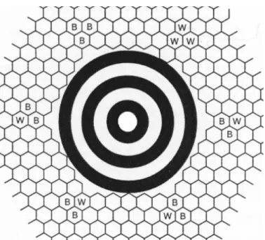
Orientation patterns give the orientation information of MaxiCode. There are 6 orientation patterns in MaxiCode, each consists of 3 modules. These patterns surround the finder pattern with the position in 1, 3, 5, 7, 9, 11 O’clock. From the aspect of the finder pattern, the angle between two neighboring patterns is 60º. In each pattern, there is a module nearest to the outside circle of the finder pattern. The distance between the outside circle and this nearest module is the length of a single module. Figure 2.6 shows an example of the orientation patterns relative to the finder pattern.

Fig. 2.6 The orientation patterns relative to the finder pattern, the orientation patterns are marked by W and B.

2.1.5 Quiet Zone

Each MaxiCode is surrounded by four quiet zone boarders. Each boarder consists of several long white runs, and the number of white runs is the length of a single module. Figure 2.7 shows an example of the quiet zone.

Fig. 2.7 An example of the quiet zone surrounded by the red dotted lines. quiet zone

2.2 Image Binarization

The image binarization plays an important role in the decoding system. A good binary thresholding method can reduce the degradation of poor quality image under an unstable lighting environment. Before thresholding, we convert the image into gray level by using 16 ) , ( * 098 . 0 ) , ( * 504 . 0 ) , ( * 257 . 0 ) , (i j = R i j + G i j + B i j + g

,

where R(i,j) denotes the red value at pixel (i,j), G(i,j) denotes the green value at pixel

(i,j) and B(i,j) denotes the blue value at pixel (i,j). In our system, an image is divided

into several subimages with size 64 x 48, and a local thresholding algorithm is applied to each subimage. Figure 2.8 shows an example of a subimage. We use Sobel operation to extract the edge point in a subimage, and the information of these edge points are used to determine the threshold value.

2.2.1 Edge point extraction

One of the features of barcodes is that most of the barcode’s color is black, and the barcodes are printed on white papers. This feature makes barcode’s edge recognizable even under extremely light, dark or other unbalanced lighting conditions. Weszka et al. [9] proposed a method to extract the edge points of an image. By the concept proposed by Weszka, we use Sobel operators (see Figure 2.9) to extract edge points. The Sobel value G of each pixel (i,j) in the subimage is defined as

y x G G G= + , where )) 1 , 1 ( ) , 1 ( 2 ) 1 , 1 ( ( + − + + + + + = g i j g i j g i j G_x )) 1 , 1 ( ) , 1 ( 2 ) 1 , 1 ( ( − − + − + − + − g i j g i j g i j , and )) 1 , 1 ( ) 1 , ( 2 ) 1 , 1 ( ( − + + + + + + = g i j g i j g i j G_y )) 1 , 1 ( ) 1 , ( 2 ) 1 , 1 ( ( − − + − + + − − g i j g i j g i j . (2.2)

Gx is the magnitude of horizontal gradient and Gy is the magnitude of vertical

-1 0 1 -1 -2 -1 -2 0 2 0 0 0 -1 0 1 1 2 1

Fig. 2.9 Two Sobel operators Gx and Gy.

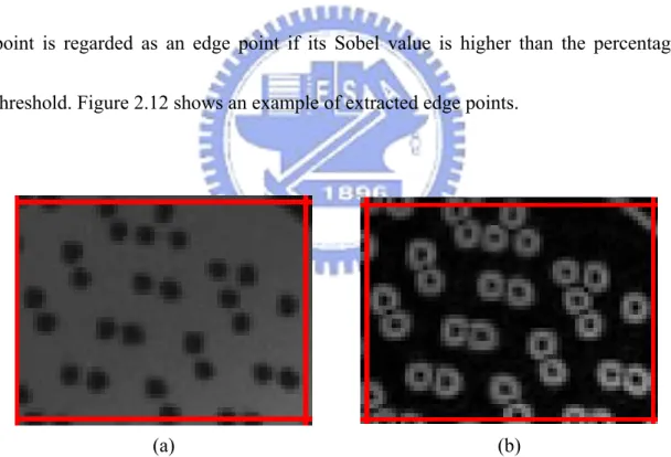
Figure 2.10 shows an example of Sobel result. The numbers of Sobel values are accumulated from low to high, and we find the value above the 80th _{percentile as a}

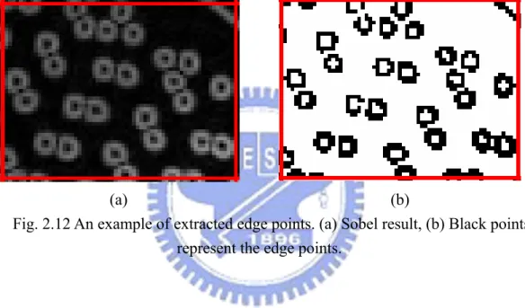
percentage threshold. Figure 2.11 shows an example of accumulating diagram. A point is regarded as an edge point if its Sobel value is higher than the percentage threshold. Figure 2.12 shows an example of extracted edge points.

(a) (b)

Fig. 2.10 An example of Sobel result. (a) Original subimage, (b) The Sobel result of the subimage.

0 20 40 60 80 100 120 0 0.2 0.4 0.6 0.8 1 Accumulating Percentage S ob el V alu e

Fig. 2.11 An example of Sobel value accumulating diagram.

(a) (b)

Fig. 2.12 An example of extracted edge points. (a) Sobel result, (b) Black points represent the edge points.

2.2.2 Minimum mean square error

After the edge points are collected, we establish the histogram of edge points, and the threshold gray value is determined by minimum mean square error method. This threshold separates the gray values into two clusters and the mean square error between the two clusters is the minimum of those among other possible two clusters. Figure 2.13 shows an example of gray value histogram of edge points. The following

Step 1. Let Min be the minimum gray value, Max be the maximum gray value and P(i) be the number of edge pixels with gray value i.

Step 2. For each value k with Min ≤ k <Max, use k to divide the histogram of the edge points into two parts. Calculate the two mean values hk,1 for the left part and hk,2

for the right part, and the mean-square error Ek through the following three formulas:

∑

∑

×

=

i

P

i

P

i

h

)

(

)

(

∑

∑

×

=

i

P

i

P

i

h

)

(

)

(

∑

∑

−

×

+

−

×

=

P

i

i

h

P

i

i

h

E

)

(

)

(

)

(

)

(

Step 3. Take the value kmin-err = argMink{Ek | Min ≤ k <Max} as the threshold.

Usually, in the background area, the gray values will not vary too much, so the square-error is low and the difference of two means (h1,h2) of both sides separated by

kmin-err will be small. Therefore, if |h1-h2| <c, where c is a pre-defined small value, the

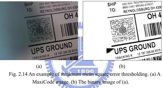
subimage is considered to be a background area. In this thesis, c is defined as 10. The background area will be filled with white pixels. Figure 2.14 shows an example of minimum mean square error thresholding.

0 5 10 15 20 25 30 0 15 30 45 60 75 90 105 120135 150 165 180 195 210 225 240 255 Gray Level Value

Nu m b er o f Pi x els

Fig. 2.13 An example of gray value histogram of edge points.

(a) (b)

Fig. 2.14 An example of minimum mean square error thresholding. (a) A MaxiCode image. (b) The binary image of (a).

2.3 Finder Pattern Location

MaxiCode has a central unique finder pattern, which is used to locate the MaxiCode. The finder pattern is made of 3 dark concentric circles and 3 included white areas. In order to extract the edge of circles of the finder pattern, the thinning morphological algorithm [8] is used. Considering the efficiency, only the central part of the image is processed, and the result of the thinned image is stored as another

Figure 2.15 shows an example of thinning result.

Fig. 2.15 An example of thinning result.

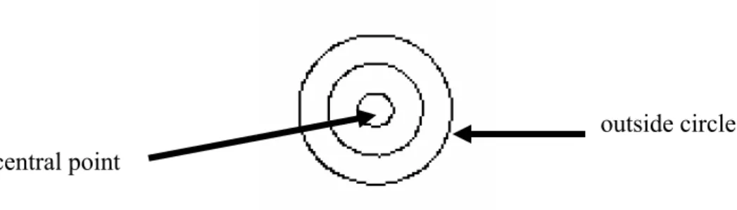
We extract the black connected component in the thinning area, and calculate the size of each component. Since the finder pattern occupies most part of the area, we can easily recognize the component of the finder pattern by the size. Figure 2.16 shows a thinned finder pattern example. We pick the component containing most pixels as the outside circle of the finder pattern. By averaging the coordinates of all pixels in this component, we can determine the coordinates of the central point of the finder pattern.

Fig. 2.16 A thinned finder pattern example with outside circle located. outside circle central point

2.4 Orientation Correction

The reading direction of MaxiCode is not limited because the orientation patterns give the position information. Figure 2.17 shows the location of orientation patterns and Figure 2.18 shows some examples of MaxiCode images taken from different directions. We propose an algorithm to detect the orientation pattern. This algorithm extracts the length of a single module, and finds the orientation patterns by scanning around the finder pattern. After the orientation patterns are found, the image is rotated into the right position.

Fig. 2.17 The location of orientation patterns marked by W and B. W is the white module and B is the black module.

2.4.1 Counting single module length

The orientation patterns are constructed by the basic modules of MaxiCode (See Fig. 2.17). The length of a single module can be used to detect the position of orientation modules. In order to calculate the length of a single module, we use a statistical method to find out the most possible length. We calculate the black run-lengths in the middle part of the image by horizontal scanning. The length of black runs on the scan line will be recorded. For efficiency, the scanning horizontal line’s frequency has a 3 pixels step size. Figure 2.19 shows an example of horizontal scanning.

(a)

(b)

Fig. 2.19 An example of horizontal scanning. (a) The horizontal scanning lines. (b) The step size of scanning lines.

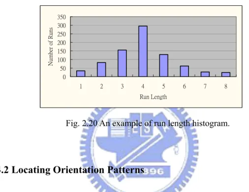
The histogram of black runs’ length will be analyzed to extract the length of a single module. Figure 2.20 shows an example of the run length histogram. Generally, we choose the peak value in the histogram as the result. For avoiding local maximum

value influencing the correct solution, we take 3 values as a group to smooth the histogram. We compare each group by their sum, and the average value of the group with the maximum sum will be taken as the length of a single module.

0 50 100 150 200 250 300 350 1 2 3 4 5 6 7 8 Run Length N um be r of Runs

Fig. 2.20 An example of run length histogram.

2.4.2 Locating Orientation Patterns

There are six orientation patterns in MaxiCode, and in this thesis, we only use four of them to correct the orientation. The patterns in positions of 3 O’clock, 5 O’clock, 9 O’clock and 11 O’clock are used. Figure 2.21 shows the corresponding patterns.

We notice that the patterns in 5 and 11 O’clocks both have two continuous black modules lying on the same line crossing the center point of the finder pattern, so we use this feature to find these two orientation patterns. We take the central point of the finder pattern as the original point, and generate the scanning line from the original point with different angles. Figure 2.22 shows the concept of scanning lines. We generate 360 lines with angles from degree 0º to degree 359º. The length of white runs and black runs in each scanning line are recorded. We remove the first 6 runs of each line since they are caused by the finder pattern, then we start to analyze the remaining runs.

Fig. 2.22 The concept of scanning line.

2.4.2.1 Orientation pattern runs analysis

pattern runs in each scanning line.All runs appearing in the same scanning line are grouped into a run set. We prune the run sets by following rules:

Rule 1. The length of the first white run in a run set should be less than or equal to the length of a single module.

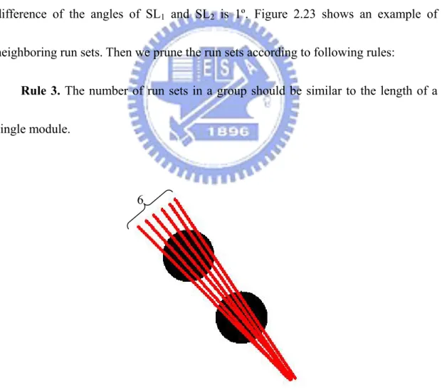
Rule 2. The number of black runs in a run set should be more than or equal to 2. Secondly, we group the neighboring run sets in the remaining run sets. Note that two run sets appearing in two scanning lines SL1 and SL2 are called neighbors, if the

difference of the angles of SL1 and SL2 is 1º. Figure 2.23 shows an example of

neighboring run sets. Then we prune the run sets according to following rules:

Rule 3. The number of run sets in a group should be similar to the length of a single module.

Fig. 2.23 An example of a group of neighboring run sets with 6 run sets. 6

Next, we check the symmetry of the remaining run set. The orientation patterns in 5 and 11 O’clock are symmetrical, that is, the difference of the angles of their scanning lines should be 180º. We prune the run sets by their symmetry according to following rules:

Rule 4. If a run set belongs to the orientation patterns, there should exist a symmetrical run set in the remaining run sets.

After these pruning steps, we may have several pairs of run set groups. Figure 2.24 shows an example of pruning result. Next, we use the feature of the orientation patterns in 3 and 9 O’clock to prune run set groups. In these two patterns, the module nearest to the finder pattern is always black, and the angles between 3 to 5 O’clock, 9 to 11 O’clock are both degree 60º. Figure 2.25 shows an example of finding 3 and 9 O’clock patterns. Therefore, we prune the group of run sets by following rules:

Rule 5. For a pair of groups of run sets, locate the first black module in the degree plus 60º for the first run set of each group. The distance from the finder pattern to these two black modules should be the same.

Figure 2.26 shows an example of the distance from the finder pattern to a black module.

(a) (b)

Fig. 2.24 An example of pruning result. (a) The original image. (b) The remaining run set groups pointed out by the arrows.

Fig. 2.25 An example of finding 3 and 9 O’clock patterns. The arrows point out the 3 and 9 O’clock orientation patterns.

By these rules, the two black modules of orientation patterns in 5 and 11 O’clocks are extracted. The final step is to identify the exact positions (5 or 11 O’clock) of the pair of two black modules. Note that the third module of the orientation pattern is white in 5 O’clock and it is black in 11 O’clock. According to this phenomenon, we generate a clockwise scanning arc to check the color of the third module. We use the finder pattern center as the center point and the middle point of the two black modules as the starting point of the arc. The radius of the arc is the distance from the central point of the finder pattern to the central point of the two black modules. Figure 2.27 shows an example of scanning arc. By the color of the third module, the exact position of the two black modules can be determined.

(a) (b)

Fig. 2.27 A example of the scanning arc. (a) The scanning arc crossing the third module of the 11 O’clock orientation pattern. (b) The scanning arc crossing the third

module of the 5 O’clock orientation pattern. center point

starting point

starting point center point

Finally, we rotate the image of MaxiCode to the right position according to the found orientation patterns. Figure 2.28 shows an example of rotated MaxiCode image.

(a) (b)

Fig. 2.28 An example of the rotated MaxiCode image. (a) Original image. (b) Rotated image.

2.5 Code Shape Rectification

The MaxiCode image could have a deformed shape since the position between the barcode and the camera mobile phone is not paralleled. Figure 2.29 shows some examples of deformation. In our system, slight deformation of MaxiCode image can be recovered. Inverse perspective transformation is often used to rectify the code shape. However, the four corner points of MaxiCode should be extracted before using inverse perspective transformation. Thus, we provide an algorithm to extract the boarders of the MaxiCode, and take the intersection points of boarders as the corner

Fig. 2.29 Some examples of MaxiCode image deformation.

2.5.1 Boarder Extraction

In the specification of MaxiCode, every MaxiCode is surrounded by a quiet zone boarder. The color of quiet zone is white, and the width of quiet zone equals to the length of a single module. In our algorithm, the quiet zone will be roughly extracted. In the region surrounded by the quiet zone, the most suitable boarder of MaxiCode will be determined.

2.5.1.1 Quiet Zone Detection

To find the quiet zone, the objective is to find four white runs surrounding the MaxiCode. Each of the white run should be a long run and the nearest run to the MaxiCode. We horizontally and vertically scan from the central point of the finder pattern, and find the first appearance of a group of long white runs. If the long white runs continually appear with number 2 times of the length of a single module, we recognize it as the quiet zone. Figure 2.30 shows an example of quiet zone. The quiet

zone can be regarded as the rough boarder of the MaxiCode, and then we extract the precise MaxiCode boarders in the region surrounded by the quiet zone.

Fig. 2.30 An example of quiet zone marked by red color.

2.5.1.2 Swing to find boarder

In order to use inverse perspective transformation, we need to find the four corner points of MaxiCode precisely. We find the nearest point to each rough boarder, and take this point as the pivot. Then we generate scanning lines which swing with this pivot, and the swinging angle ranges from -3.0º to 3.0º degrees, adding 0.2º degrees per move. Figure 2.31 shows an example of swinging scanning lines. We take the scanning line touching the most modules as the precise boarder. Figure 2.32 shows an example of MaxiCode with extracted boarder. Finally, we take the four intersection

a group of white runs

Fig. 2.31 An example of swinging scanning lines.

Fig. 2.32 An example of MaxiCode with extracted boarder.

2.5.2 Inverse Perspective Transformation

The following equations calculate coefficients of perspective transformation [7] which maps vertexes (xi,yi) to vertexes (ui,vi) (i=1,2,3,4):

22 21 20 02 01 00 c y c x c c y c x c u i i i i i _{× + × +} + × + × = , (2.6) and 22 21 20 12 11 10 c y c x c c y c x c v i i i i i _{× + × +} + × + × = . (2.7)

Coefficients are calculated by solving linear system: pivot

⎥ ⎥ ⎥ ⎥ ⎥ ⎥ ⎥ ⎥ ⎥ ⎥ ⎥ ⎦ ⎤ ⎢ ⎢ ⎢ ⎢ ⎢ ⎢ ⎢ ⎢ ⎢ ⎢ ⎢ ⎣ ⎡ = ⎥ ⎥ ⎥ ⎥ ⎥ ⎥ ⎥ ⎥ ⎥ ⎥ ⎥ ⎦ ⎤ ⎢ ⎢ ⎢ ⎢ ⎢ ⎢ ⎢ ⎢ ⎢ ⎢ ⎢ ⎣ ⎡ ⎥ ⎥ ⎥ ⎥ ⎥ ⎥ ⎥ ⎥ ⎥ ⎥ ⎥ ⎦ ⎤ ⎢ ⎢ ⎢ ⎢ ⎢ ⎢ ⎢ ⎢ ⎢ ⎢ ⎢ ⎣ ⎡ − − − − − − − − − − − − − − − − 3 2 1 0 3 2 1 0 21 20 12 11 10 02 01 00 3 3 3 3 3 3 2 2 2 2 2 2 1 1 1 1 1 1 0 0 0 0 0 0 3 3 3 3 3 3 2 2 2 2 2 2 1 1 1 1 1 1 0 0 0 0 0 0 1 0 0 0 1 0 0 0 1 0 0 0 1 0 0 0 0 0 0 1 0 0 0 1 0 0 0 1 0 0 0 1 v v v v u u u u c c c c c c c c v y v x y x v y v x y x v y v x y x v y v x y x u y u x y x u y u x y x u y u x y x u y u x y x , (2.8)

where cij are matrix coefficients, c22 = 1.

Let f(x,y) represent the pixel value in position (x,y) in the rectified image, and g(u,v) represent the pixel value in position (u,v) in the original image. The rectified

image is mapped from the original one by the following equation:

⎟⎟ ⎠ ⎞ ⎜⎜ ⎝ ⎛ + + + + + + + + = = 22 21 20 12 11 10 22 21 20 02 01 00 _, ) , ( ) , ( c y c x c c y c x c c y c x c c y c x c g v u g y x f (2.9)

The resolution of the rectified image is defined as 210 x 200. Figure 2.33 shows an example of rectified MaxiCode image.

(a) (b)

2.6 Data Extraction

To decode the information embedded in the MaxiCode, we need to extract the data from modules. There are 33 rows of modules in a MaxiCode, so we separate the image into 33 parts in rows, and recognize the modules in each row by run length counting. After all modules being recognized, the data are decoded by the specification of MaxiCode. Finally, the result of decoding will be shown on the screen of the mobile phone.

2.6.1 Module run length counting

In a MaxiCode, there are 30 modules in each odd row and 29 modules in each even row. Black modules represent 1 and white modules represent 0. We calculate the white runs and black runs in each row, and analyze how many modules in each row. The finder pattern is removed at the beginning of this stage to avoid influencing the counting of run lengths.

In each row, we choose the scanning line which contains the most number of black pixels as the central line, and the data is regarded as the major data which is obtained from the range of adding and minus 1-pixel on the central line. We extract the horizontal projection length of the major data as black run length, and we take the length between black runs as white run length. Figure 2.34 shows a horizontal

projection example.

Fig. 2.34 A horizontal projection example.

The theoretical length of each module is 7, since the width of the rectified image is 210, and each odd row contains 30 modules. Based on this fact, the black and white run lengths are recognized by the following rules:

Rule 1. If the black run length is greater than 1, a black module is generated, and the run length minus 7.

Rule 2. If the white run length is greater than 5, a white module is generated, and the run length minus 7.

The runs of the finder pattern will be skipped during recognition. Since the start position of the first module of each even row is half module behind that of each odd row, the first white run of each even row will first minus 3.

Finally, the generated modules will be decoded following the specification of projected length central line

CHAPTER 3

EXPERIMENTAL RESULTS

In order to evaluate the decoding rate of the proposed system, we generate 20 MaxiCode sample images. The camera mobile phone we used is Sony Ericsson C902 [10]. We build the system in J2ME platform [11]. In the experiment, we construct two environment conditions, one is under controlled and another one is not. For each image, the average decoding time is 14 seconds in the mobile phone, and less than 1 second in the PC (AMD64 3200+ CPU; 2.0Ghz; 1GB memory). An image is said to be decodable if the extracted data can be recovered by the Reed-Solomon code. If the amount of the error data is over the tolerance of the Reed-Solomon code, a request to take another shot will be sent.

3.1 Controlled Environment

In the controlled environment, the pictures of each sample will be taken under different conditions. Rotation, different lighting sources, oblique and different focal distance are the controlled events for testing the system. Only one of the events is adjusted in each testing.

3.1.1 Rotation

In the rotation effect testing, each sample will be taken shot in 0º, 45º, 90º, 135º, 180º, 225º, 270º and 315º degrees. The lighting condition is stable and the camera is parallel to the MaxiCode samples. The distance between the camera phone and the MaxiCode samples is 7.5 cm, and the camera phone is turned to the Marco mode. Table 3.1 shows the decoding rate in each rotation angle. Figure 3.1 shows some examples of the images taken under different rotation angles. Under different rotation angles, the decoding rate of the system is 100%. Experimental results show that the system is capable of decoding MaxiCode images with rotations.

Table 3.1 The decoding rates under different rotation angles. Rotation angle Decoding Rate

0º 100% 45º 100% 90º 100% 135º 100% 180º 100% 225º 100% 270º 100% 315º 100%

(a) (b)

(c) (d)

(e) (f)

(g) (h)

Fig. 3.1 Some examples of the images taken under the different rotation angles. (a) 0º. (b) 45º. (c) 90º. (d) 135º. (e) 180º. (f) 225º. (g) 270º. (h) 315º.

3.1.2 Different Lighting Sources

In the different lighting sources testing, each sample will be taken shot outside and inside. In outside, the source of lighting is sunlight. In inside, the sources of lighting are fluorescent lamp and desk lamp. Another test inside is taking the pictures without any lighting source. The distance between the camera phone and the MaxiCode samples is 7.5 cm, and each sample is taken shot without rotation. Table 3.2 shows the decoding rate in each lighting condition. Figure 3.2 shows some examples of the images taken under lighting sources. Under different lighting sources, the decoding rate of the system is 100%. Experimental results show that the system is capable of decoding MaxiCode images in different lighting conditions.

Table 3.2 The decoding rates under different lighting sources. Lighting Source Decoding Rate

Sunlight 100%

Fluorescent Lamp 100%

Desk Lamp 100%

(a) (b)

(c) (d)

Fig. 3.2 Some examples of the images taken under different lighting sources. (a) Sunlight. (b) Fluorescent Lamp. (c) Desk Lamp. (d) Inside (turn off light).

3.1.3 Oblique

In the oblique effect testing, the angle between the mobile camera phone and the samples will vary from -40º to 40º, with interval 10º per move. The lighting condition is stable and the distance between the camera phone and the MaxiCode samples is 7.5 cm. Each sample is taken shot without rotation. Table 3.3 shows the decoding rate in each oblique angle. Figure 3.3 shows some examples of the images taken under different oblique angles. From the experimental results, we can see that the decoding rate is 100% with oblique angles between -20º and 20º, it decreases with oblique

angle 30º and -30º, and all the images are undecodable if the oblique angle over 40º and -40º. The poor decoding rate is caused by the deformation of the MaxiCode. Oblique angles make the shape of MaxiCode slanted in the image. Slanting makes the orientation patterns deviate from their original positions, leading the system to be unable to correct the orientation.

Table 3.3 The decoding rates under different oblique angles. Oblique angle Decoding Rate

-40º 0% -30º 70% -20º 100% -10º 100% 10º 100% 20º 100% 30º 65% 40º 0%

(a) (b)

(c) (d)

(e) (f)

(g) (h)

Fig. 3.3 Some examples of the images taken under the different oblique angles. (a) -40º. (b) 40º. (c) -30º. (d) 30º. (e) -20º. (f) 20º. (g) -10º. (h) 10º.

3.1.4 Different Focal Distance

In the focal distance testing, the distance between the camera mobile phone and samples will be adjusted. The range of distances is from 5cm to 30cm. The lighting condition is stable and the camera is parallel to the MaxiCode samples. Each sample is taken shot without rotation. Table 3.4 shows the decoding rate in each focal distance. Figure 3.4 shows some examples of the images taken under different focal distances. Experimental results show that the system works well from distance of 6cm to 30cm. In distance of 5cm, the images are all out-of-focus due to the limitation of focusing ability of camera mobile phones, and the MaxiCode is blurred in the images. Blurring makes the modules of MaxiCode distorted, resulting in that the orientation patterns cannot be extracted.

Table 3.4 The decoding rates under different focal distances. Focal Distance Decoding Rate

5cm 65% 6cm 100% 7cm 100% 8cm 100% 9cm 100% 10cm 100% 15cm 100% 20cm 100% 30cm 100%

(a) (b) (c)

(d) (e) (f)

(g) (h) (i)

Fig. 3.4 Some examples of the images taken under the different focal distances. (a) 5cm. (b) 6cm. (c) 7cm. (d) 8cm. (e) 9cm. (f) 10cm. (g) 15cm. (h) 20cm. (i) 30cm.

3.2 Uncontrolled Environment

In the uncontrolled environment, we invite 10 users to take MaxiCode pictures. For each MaxiCode sample, one picture will be taken. These users are not familiar with MaxiCode, and they are not informed to stabilize the lighting condition or the proper distance between the barcode and the mobile phone. Figure 3.5 shows some examples of the images taken by users. Under the different lighting conditions, different MaxiCode size in the image and different user’s habits, the decoding rate of

our system is 81%.

the MaxiCode in the picture. Figure 3.6 shows some examples of undecodable images. Blurring is often occurred by the users’ hand-shaking or out-of-focus when taking pictures. If an image is blurred, the shape of MaxiCode modules will distort in the binarization step. Figure 3.7 shows some examples of binarization results of undecodable images. The distortion of modules results in that the orientation patterns cannot be extracted. Another reason for undecodable images is the slanting of images. Slanting is the deformation of the entire shape of the MaxiCode in the image, and it is often caused by the oblique position between the barcode and the camera. A slanted image makes the orientation patterns deviate from their original position, leading the system to be unable to correct the orientation. Although the system can rectify the shape of MaxiCode during decoding, the slanted image still can not be recovered if the orientation patterns are missed.

The system will send a message to users if the image is undecodable, and ask users to take another shot. The number of times users take shots are recorded. In our system, a MaxiCode image can be decoded correctly by taking 1.2 pictures in average.

(a)

(b)

Fig. 3.6 Some examples of undecodable images. (a) Blurring. (b) Slanting.

CHAPTER 4

CONCLUSION

The system provides users a convenient application on camera mobile phone to decode MaxiCode. Users can take a MaxiCode image with slight restriction, and the system can decode the information correctly within a reasonable time. In the future, we will improve the system by reducing the decoding time. Furthermore, the distortion of image is the main reason of erroneous decoding, so it is the target to make the system more robust.

REFERENCES

[1] ISO/IEC 16023:2000. Information technology – International symbology specification – MaxiCode, 2000.

[2] ISO/IEC 15438:2001. Information technology – Automatic identification and data capture techniques – Bar code symbology specifications – PDF417, 2001.

[3] ISO/IEC 18004:2006. Information technology – Automatic identification and data capture techniques – QR Code 2005 bar code symbology specification, 2006. [4] http://www.ups.com

[5] E. Ottaviani, A. Pavan, M. Bottazzi, E. Brunelli, F. Caselli and M.Guerrero, “A Common Image Processing Framework for 2D Barcode Reading,” Image

Processing and Its Applications, Seventh International Conference on (Conf. Publ. No. 465), Manchester, UK, Vol. 2, pp. 652-655, Jul. 1999.

[6] Y. Tanaka, Y. Satoh and M. Kashi, “Hand-held Terminal with Multi-code Reader,”

Fujitsu scientific & technical journal, Vol. 35, Iss. 2, pp. 267-273, Dec. 1999.

[7] E. Ohbuchi, H.Hanaizumi and L. A. Hock, “Barcode Readers using the Camera Device in Mobile Phones,” Proceedings of the 2004 International Conference on

Cyberworlds, Tokyo, Japan, pp. 260-265, Nov. 2004.

[9] J. S. Weszka, R. N. Nagel and A. Rosenfeld, “A Threshold Selection Technique,”

IEEE Transactions on Computers, Vol. C-23, Iss. 12, pp.1322-1326, Dec. 1974.

[10] http://developer.sonyericsson.com [11] http://java.sun.com