以系統動態探討社會面因素對於教師評分的影響

全文

(1)國立交通大學資訊科學系碩士論文. 以系統動態探討社會面因素對於教師評分的影響 How Social Factors Influence Teachers’ Grading? A System Dynamics Approach.. 研究生：端木蘋指導教授：孫春在. 中華民國. 教授. 九十四. 年六月.

(2) 以系統動態探討社會面因素對於教師評分的影響學生：端木蘋. 指導教授：孫春在. 教授. 國立交通大學資訊科學研究所. 摘要當代學校評分的研究著重於評分準則制定的議題上、尋求一套有效的評分準則、以及比較各種評分準則的優缺點。本研究以模擬的設計角度來觀察蘊藏於教師評分的評分準則背後社會面因素影響。我們使用系統動態方法成功模擬找出評分行為模式的評分架構。我們的實驗資料來源為台灣北部某 C 大過去連續八學期的課程評分資料做為我們模型的實驗數據資料庫。本研究提出的模型建議，找出以往評分的行為模式是可行的。找出以往評分的行為模式可以有效的幫助校方理解教師評分時的想法及考量，並且提供校方評分準則的決策者ㄧ個明確的方向來改善評分準則的有效性。. 關鍵字：社會面因素、系統動態學、教師評分. i.

(3) How Social Factors Influence Teachers’ Grading? A System Dynamics Approach. Student: Ping Dwuanmu. Advisor: Dr. Chuen-Tsai Sun. Institute of Computer and Information Science National Chiao Tung University. ABSTRACT The contemporary researches of grading in school have focused on the issue of the grading standard in making the grading standard, pursuing the evaluation efficiency of the grading standard, and comparing advantages and advantages with all kinds of grading standards. This study reports on a simulation designed by using System Dynamics to see the factors influencing teachers’ grading behind the grading standard from the social point of view. The simulation succeeds in finding the grading structure of the grading pattern of behavior by using the system dynamics approach. Our research and experiment data source come from the data of evaluation of each class in the University C located at North Taiwan. Our model suggests that it is possible to find out the structure of the past grading pattern of behavior. It is good for understanding the thought of teachers’ grading and providing the grading policymaker a direction to improve the evaluation efficiency of grading. Keywords: Social Factors; Social point of view; System Dynamics; Grading structure. i.

(4) 誌謝感謝孫春在老師ㄧ次又一次不厭其煩的將我模糊的腦袋指引到正確的研究方向上，這兩年的時間，我經歷了一場出乎我意料的研究所路程，但很值得。此外，感謝碩一的一年來，室友喬文、璧如及岱伊學姊給我的鼓勵及傾聽我ㄧ肚的苦水；感謝崇源學長、芳芳學姊提供相當重要的概念及想法，使我的論文雛型越來越清晰；感謝實驗室承龍學長、同屆同學敬華、冠傑、家胤、仁鴻、其煜、健銘、喬文、東鴻、Camil，在這兩年來所有課業上的幫忙以及給我的腦力激盪和熱情的幫我找 bug，讓我順利的完成碩士論文；同時感謝下一屆可愛的學弟妹讓我在碩二忙碌的這一年來，生活還是相當開心和有趣。最後，我要感謝我可愛的老爸和特地衝回來等我畢業的老媽還有我親愛的老姊，沒有他們在背後默默的支持和叮嚀，這個論文我是寫不完的。非常感激大家陪我的這段時間。. ii.

(5) Content ABSTRACT ............................................................................................................................................ I 1. INTRODUCTION.........................................................................................................................1. 2. RELATED WORK .......................................................................................................................3. 3. 4. 5. 6. 2.1. RELATED WORKS TO GRADING................................................................................................3. 2.2. SYSTEM DYNAMICS ...............................................................................................................3. THE MODEL................................................................................................................................5 3.1. THE FOUR ASSUMPTIONS IN OUR MODEL ................................................................................6. 3.2. THE SOCIAL INFLUENCED STRUCTURE ....................................................................................7. 3.3. THE EQUATION OF OUR MODEL ...............................................................................................9. 3.4. FRAMEWORK OF THE SYSTEM...............................................................................................10. THE EXPERIMENTS................................................................................................................ 11 4.1. THE DATA ............................................................................................................................. 11. 4.2. DESCRIPTION FOR OUR EXPERIMENTS ..................................................................................12. THE RESULTS ...........................................................................................................................13 5.1. ABOUT THE GRADING PATTERN OF BEHAVIOR .......................................................................13. 5.2. THE GRADING STRUCTURE ...................................................................................................16. 5.3. ANALYSIS OF THE RESULTS ...................................................................................................21. CONCLUSIONS .........................................................................................................................24. iii.

(6) List of Tables Table 1 Definition of four assumption ...........................................................................6 Table 2 Relationships among the assumptions and the grading ....................................8 Table 3 Relationships among the assumptions and the grading ..................................17 Table 4 Relationship among the assumptions and the grading ....................................20. List of Figures FIG. 1 THE CAUSAL LINK ............................................................................................................................5 FIG. 2 THE SIGN OF A CAUSAL LINK ............................................................................................................5 FIG. 3 INPUT OF THE ASSUMPTION ..............................................................................................................7 FIG. 4 THE FRAMEWORK OF THE SYSTEM STRUCTURE ................................................................................9 FIG 5 THE SYSTEM FRAMEWORK .............................................................................................................10 FIG. 6 THE RESULT OF THE AVERAGE OF COLLEGE OF HUMANITIES .........................................................14 FIG. 7 THE RESULT OF THE HIGHEST SCORE OF COLLEGE OF HUMANITIES ...............................................15 FIG. 8 THE RESULT OF THE AVERAGE SOCIAL SCIENCES ...........................................................................15 FIG. 10 THE BAR CHART OF THE ORDER OF SOCIAL FACTORS INFLUENCES ................................................17 FIG. 11 THE CAUSAL LOOP DIAGRAM OF SYSTEM DYNAMICS ...................................................................18 FIG. 12 THE BAR CHART OF THE ORDER OF SOCIAL FACTORS INFLUENCES ................................................19 FIG. 13 THE CAUSAL LOOP DIAGRAM OF SYSTEM DYNAMICS ...................................................................20 FIG. 14 THE CORRELATIONS EXAMINED BY ANOVA................................................................................21 FIG. 15 SOME EVALUATIONS WE PREVIOUSLY VERIFIED BY THE STATISTICS ..............................................23 FIG. 16 ANOTHER NEGATIVE CORRELATION WE VERIFIED BY THE STATISTICS ..........................................23. iv.

(7) 1 Introduction It focused on how to develop a precise, reliable, fair grading system for representing the study achievements of students in the past researches of teachers’ grading. However, most professionals in Education think the contemporary grading standards we use are still not appropriate. (Guskey, T. R., 2001). An analysis on the social mechanisms affecting the grading of university students was conducted using system dynamic simulation model to demonstrate the possible uses, constraints and limitations, and applications of simulation-based research approaches.. The grading guidance can show the concrete level which school leaders want to pay attention to (Chicago Board of Education, 2000.) An effective grading evaluation has a good feedback to a student and provides with its identification. However, the phenomenon has been observed that the scores got by students are higher and higher, recently. If the definition of the range to the perfect score isn’t change and under the circumstance of the grade given by teachers move upper and upper, this is going to bring about the problem that the gap is getting smaller and smaller between the perfect score and grading. At the same time, it means the score differential of every individual among them is getting little and little. Human can not see something meaningful or different from extremely small number. What the worst is even we verify it by statistics, there is no significant difference, probably. This causes that the grading lose its identification.. Based on the data of evaluation of each class in the C University from 1985 to 2002, we built a dynamic system model to explain the changes and trends of grading. 1.

(8) in higher education.. The model includes the effects of various factors on university. teachers’ grading tendency, including the substitution of a class, the popularity of a teacher, the introducing of the teaching evaluation system, and the changes of students enrolled in a course. The model could be used to depict the complicated social environments of grading processes of teachers.. Because of the specific observation to the trend of the grading we want to take and the particular time-accumulated relationships of the influences, the definition of system dynamics and our grading dynamics model matches very much. The system dynamics methods have been used for over thirty years (Forrester, J.W., 1961) and are now well established. Besides, system dynamics requires that we move away from looking at isolated events and their causes (usually assumed to be some other events), and start to look at the organization as a system made up of interacting parts. It is the best method for us to build our model with system dynamics.. The next section outlines some researches made about grading and a brief definition of system dynamics. The third section of the study describes the definition with the assumptions and structure in our model completely. The fourth section of the study describes the detailed data we have and our experiments. The fifth section of the study describes the results of our experiments, analyses to the results, and verification of our model. The final section uses the social factors influenced structure to suggest some conclusions about the educational guiding principle to the policymakers.. 2.

(9) 2 Related Work 2.1 Related works to grading Teachers need a clear, understood grading system to present students’ study achievements when reporting the students’ scores (Guskey, T. R., 2001).. Many teachers make grading by some combinations of rules, and use only a number or a level to present students’ achievements. In fact, the grading contains lots of meanings (Brookhart, S. M., 1993), including the hidden social influences behind the rules like the comparison among teachers, the population of a course, the welcome degree of a course, the evaluation to the teacher and the course, the seniority of a teacher, the pressure comes from regulations of the school , and so on. However, there have been few articles discuss how these social influences affect teachers grading.. Recently, researches focus on some points about the grading most in grading standard aspects: for instance, how to make efficient grading standards (Hong-Mei, Cheng , 2002), define the motivation of grading(Enger, S. K. and Yager, R. E., 2001), find a boarder policy context which margins teacher assessment (Hall, K. and Harding, A., 2002), a system of the teacher evaluation(Milanowski, T. and Heneman, H. G., 2001), how local school leaders make sense to evaluate teachers and teaching(Halverson, R., Kelley, C. and Kimball, S., 2004).. 2.2. System Dynamics. Besides, System dynamics has long been used (Mahadevan, B., 2000) and there 3.

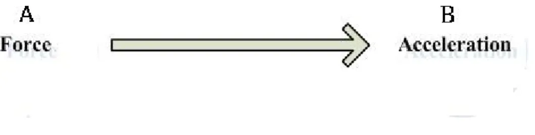
(10) have been lots of different issues discussed in system dynamics approach. Some issues about the mobile telecommunication (Tung B. & Claudia L., 1996.), management (Erik & Ann & Kim, 1997), business models (Mahadevan, B., 2000), bionomics, and financial models. With all the above-mentioned examples, it is a great help for us to build our model by the system dynamics approach.. We briefly discuss the main ideas and concepts of the system dynamics approach. The central concept to system dynamics is understanding how all the objects in a system interact with one another (MIT System Dynamics in Education Project, SDEP). What system dynamics attempts to do is understand the basic structure of a system, and thus understand the behavior it can produce. A system can be anything from a steam engine, to a bank account, to a basketball team. The objects and people in a system interact through "feedback" loops, where a change in one variable affects other variables over time, which in turn affects the original variable, and so on. There are three main elements in system dynamics: events, causal links, and signs (Craig, W. K., 1998). In general, we use the arrow to represent the relation among the events. An arrow linking two related events we call it a causal link (see Figure 1), when an event of a system indirectly influences itself in the way discussed for Inventory in the preceding paragraph, the portion of the system involved is called a feedback loop or a causal loop. Feedback is defined as the transmission and return of information (Richardson, G. P. and Pugh III, A.L., 1981).. 4.

(11) Fig. 1 The causal link There are two kinds of sign: positive and negative. If either A adds to B or a change in A produces a change in B in the same direction, the causal link is positive. Oppositely, If either A subtracts from to B or a change in A produces a change in B in the opposite direction, the causal link is negative (see Figure 2).. Fig. 2 The sign of a causal link. 3 The Model Our model focuses on finding the social factors in teachers’ grading and how social factors influence teachers’ grading. The model is discussed below. This is followed by a brief description of the full model.. 5.

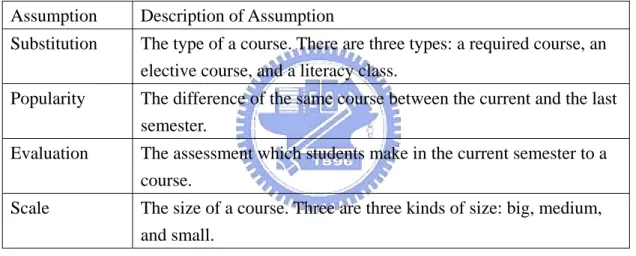
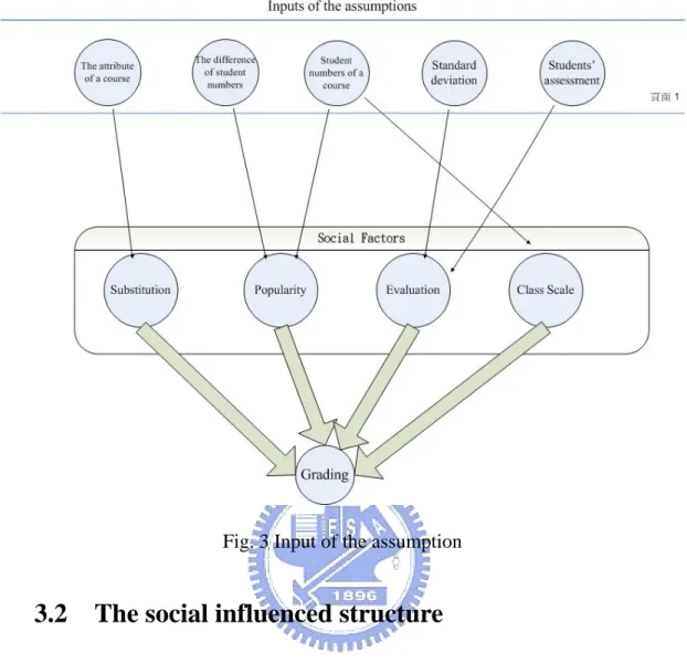
(12) 3.1. The four assumptions in our model. According to original items we have and another calculated statistics of the data (see the Appendix A), we assumed four assumptions (see Table 1) of the social factors that affect grading which we concerned about to define our model. The grading of our definition means the scores that a teacher gives in one semester. Because all those data have different values with different range, we normalized the four assumptions and all inputs of the four assumptions to make sure their consistency. Then we can draw a frame to see the inputs of the assumptions (see Figure 3). Assumption. Description of Assumption. Substitution. The type of a course. There are three types: a required course, an elective course, and a literacy class.. Popularity. The difference of the same course between the current and the last semester.. Evaluation. The assessment which students make in the current semester to a course.. Scale. The size of a course. Three are three kinds of size: big, medium, and small. Table 1 Definition of four assumptions. Our model built on the relationship among the assumptions and the grading.. 6.

(13) Fig. 3 Input of the assumption. 3.2. The social influenced structure. Based on the definition we made, we can show a matrix of the relationship among the assumptions and the grading (see Table 2). The size of the matrix is 5*5 and therefore comes 25 relationships including the two-way influence between every two elements (e.g. relation between No 3 and No 11 is a relationship with symmetry). After finishing the definition of the matrix, we use both statistics and genetic algorithms (Darrell Whitley, 1993) to find what kind of those influences belongs to.. 7.

(14) Grading. Substitution. Popularity. Evaluation. Scale. Grading. (1). (6). (11). (16). (21). Substitution. (2). (7). (12). (17). (22). Popularity. (3). (8). (13). (18). (23). Evaluation. (4). (9). (14). (19). (24). Scale. (5). (10). (15). (20). (25). Table 2 Relationships among the assumptions and the grading The relationship among the assumptions and the grading We defined five kinds of relationships. They are presented in the symbol of ‘+’, ‘-’, ‘X’, or numbers. The symbol ‘+’ means a factor affects another factor with a positive influence. The symbol ‘-’ means a factor affects another factor with a negative influence. We use the symbol ‘X’ by meaning that we are sure the relationship can’t be influenced by another. The relationship shown in a number represents especially the order of the influence among the four assumptions, except the number ‘0’. We use it to stand for a influence which causes no influence to another factor we find in our experiment. Then we can construct the framework of the system structure with all the factors and the influences among them (see e.g. Figure 4).. 8.

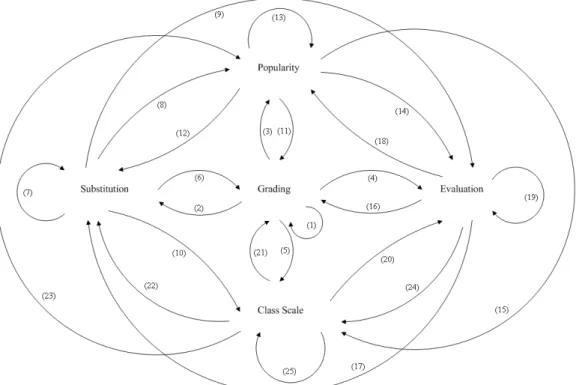
(15) Fig. 4 The framework of the system structure The framework of the system structure with all the factors and the influences among them.. 3.3. The equation of our model. To describe that how social factors influence the grading, our model can be represented as: Grading(t+1)＝F [Sub(t ), E (t ), P(t ), Sc(t )] Sub(t) ＝ a ∗ Substituti on (t ) E(t) ＝ b ∗ Evaluation (t ) P(t) ＝ c ∗ Popularity (t ) Sc(t) ＝ d ∗ Scale (t ) Where Grading (t+1) is the number of Grading at any time t+1 and equal to the number of the function F,. 9.

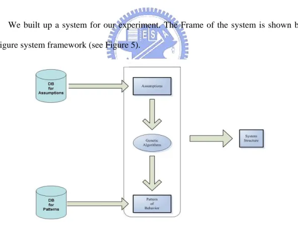
(16) Sub (t) is the number of Substitution at any time t and equal to the number multiplying a coefficient a, E (t) is the number of Evaluation at any time t and equal to the number multiplying a coefficient b, P (t) is the number of Popularity at any time t and equal to the number multiplying a coefficient c, Sc (t) is the number of Scale at any time t and equal to the number multiplying a coefficient d, We assume that the initial time is t = 0.. 3.4. Framework of the system. We built up a system for our experiment. The Frame of the system is shown by Figure system framework (see Figure 5).. Fig 5 The system framework. The system includes a database, a system kernel, and the output of result. The database provides the input values of system parameters. The system kernel contains 10.

(17) the elements (In our model, the elements mean the social factors and the grading) which is used to form the system structure and the pattern of behavior to the specific system structure. The practical pattern of behavior is supported by the same database as the one providing the input values of system parameters. We use Genetic Algorithms to tune the direction and the sign of elements affected mutually, making the pattern of behavior produced by the system structure tuned with Genetic Algorithms to fit the practical pattern of behavior or at least to fit the trend of the practical pattern of behavior. We’ll get an output of our system after Genetic Algorithms done. The results we get comprise the causal link and the sign of the causal link and they are the system structure to the pattern of behavior found by our model. We use the system dynamics approach to build up our grading model. The system dynamics approach uses lots of symbols but not a differential equivalence to represent changes in the system status. There will be some stocks and flow diagrams in the approach. We use the basic First Model in our study to find the basic grading structure. After that, we can continue discussing it with higher level models. Besides, we use statistics to provide the analysis and verification of our assumption. We choose the genetic algorithm to adjust values of parameters because the genetic algorithm is more flexible when we want to modify amount of parameters.. 4 The Experiments 4.1. The data. The data of our research comes from the C University in the north Taiwan. In order to guarantee the correctness and completeness in our data, we filter out some of them which are ambiguous, and extracted a continued eight semester data to be our 11.

(18) database. The amounts of data that we picked up are 5806. And we have 25 properties (see Appendix A) for the data, containing 12 properties of them in the original data and the others from gathering statistics in the original data. We used these properties to be the foundation to support our four assumptions. In addition, we separate the data by the property of the academy, because the values in this property can not be quantified in numbers and compared with each other. There are five academies in the data we got, and they are: College of Electrical Engineering & Computer Science (ES), College of Engineering (E), College of Science (S), College of Management (M), and College of Humanities and Social Sciences (HS). They all have different patterns of behavior under different definition of Grading.. 4.2. Description for our experiments. A teacher will give every student a score at the end of the semester. However, only to look at so many scores in a course we can’t see some information in them or something meaningful in those scores. Hence, statistic is a good tool to find some basic phenomena in data and we use statistic to classify a variety of grading. We will discuss what and how social factors influence the grading and the feedback of the grading to social factors by finding their structures in two significant statistics in our experiment in this chapter (we do some more experiments please to see the appendix). The two statistics are: the average and the highest score.. The average (the arithmetic mean): The arithmetic mean is the most frequently used by far. The arithmetic mean is provided with three essential meanings: firstly, the arithmetic mean can simplify all values of a group becoming one single value, the. 12.

(19) function of the simplification, precisely speaking. We simplify lots of scores in one course, so that we can see changes of a course in the continuous eight semesters. Secondly, the arithmetic mean can stand for a mean standard of a group, namely, the function of representation. The five academies had their some kind of style of themselves. At last, after simplifying the arithmetic mean, here comes a value which represents the function of representation to be a great help to compare with two groups or over two groups. The average is the most basic statistic. Some other advanced statistics are calculated with this statistic, so it is important for us to find its structure to social factors influences first. We can observe the dissimilar appearance among the five academics and explain them by their architecture we found in our experiment.. The highest score: The highest score in a course. Looking into the highest score and average, we can see if they have similar trends. If the answer is yes, we are interested in if their structures of social influences are similar, too. On the contrary, we are desired to know the reasons from the social influences. And then we used our model to run the two grading experiments.. 5 The Results We will display the results of the two grading which we mentioned above in our experiment and analyze their social factors influenced structures. By the equation of Grading(t+1)＝F [a ∗ Substitution(t ), b ∗ Evaluation(t ), c ∗ Popularity(t ), d ∗ Scale(t )] We can duplicate the grading trend and find the structure of it.. 5.1 About the grading pattern of behavior 13.

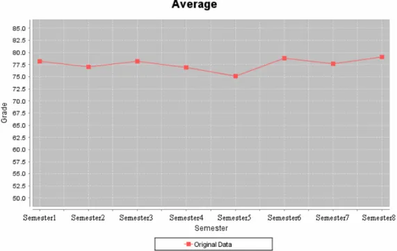
(20) Figure 6 and 8 shows the result of the average of College of Humanities and Social Sciences, and figure 7 and 9 shows the result of the highest score of College of Humanities and Social Sciences in our experiment of simulation. Our results fit well with the trend of the grading curve of College of Humanities and Social Sciences (the other Colleges are as well, too. See Appendix A.) It has been proved that if the model can reproduce the data, the model is reliable and effective (Jacobsen, C. & Bronson, R., 1995). Fig. 6 The result of the average of College of Humanities The average of College of Humanities and Social Sciences. 14.

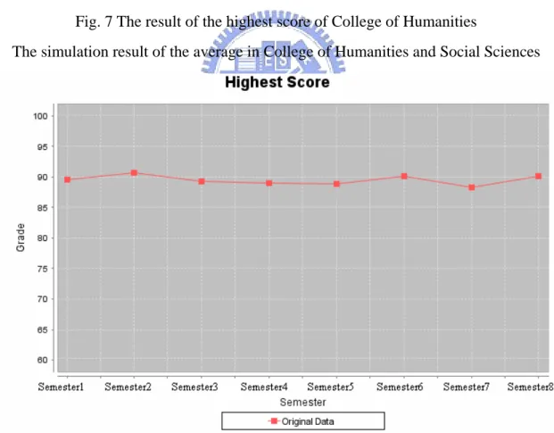
(21) Fig. 7 The result of the highest score of College of Humanities The simulation result of the average in College of Humanities and Social Sciences. Fig. 8 The result of the average Social Sciences The highest score of College of Humanities and Social Sciences. 15.

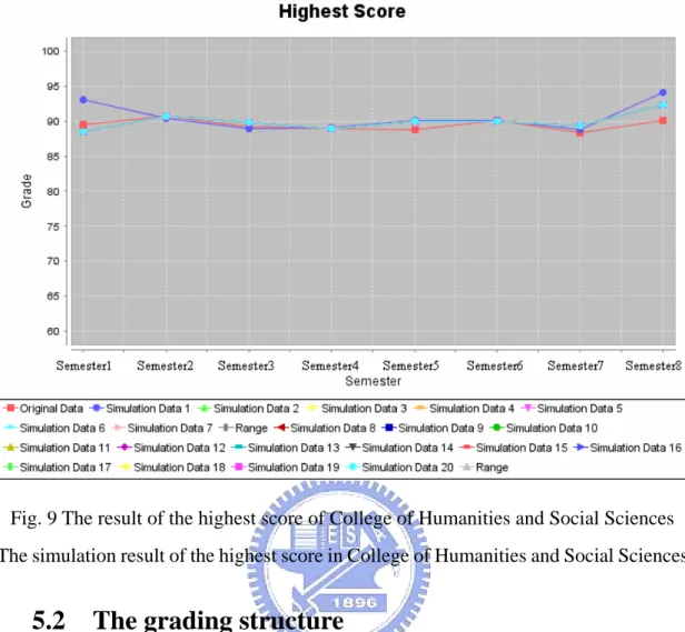
(22) Fig. 9 The result of the highest score of College of Humanities and Social Sciences The simulation result of the highest score in College of Humanities and Social Sciences. 5.2. The grading structure. In our simulation, the order of Sub(t), E(t), P(t), and Sc(t) of the average in the five academies are: HS: Sc(t) > P(t) > Sub(t)= E(t) M:. Sc(t) > P(t) > Sub(t)= E(t). S:. P(t) > Sc(t) > Sub(t) > E(t). E:. P(t)> Sub(t)= E(t) > Sc(t). ES:. P(t)> Sub(t)= E(t) > Sc(t). We can use a bar chart to see the order of social factors influences more clearly in Figure 10.. 16.

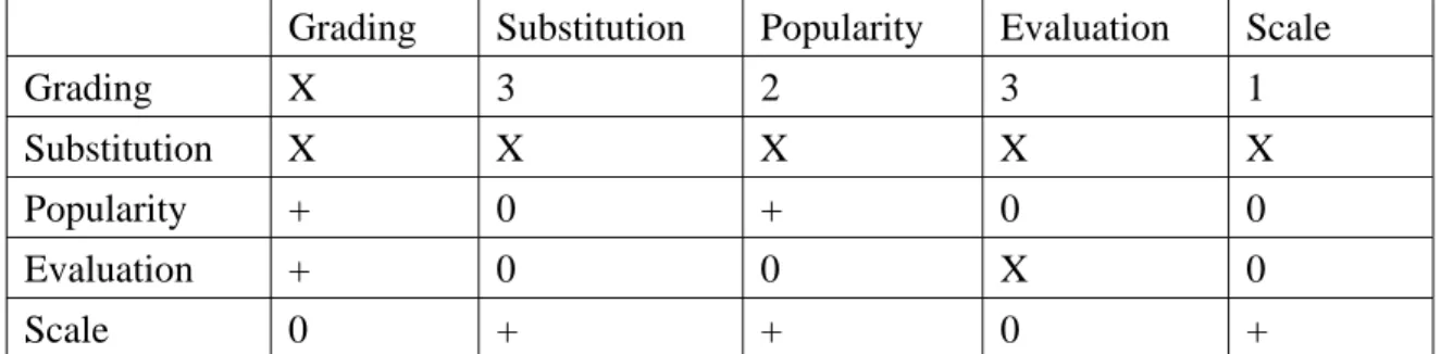
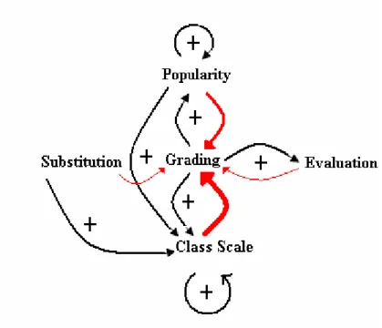
(23) Fig. 10 The bar chart of the order of social factors influences The order of social factors influences of the average in the five academies. According to the matrix of the relationship among the assumptions and the grading (See Table 3), we can draw the causal loop diagram of system dynamics (See Table 11).. Grading. Substitution. Popularity. Evaluation. Scale. Grading. X. 3. 2. 3. 1. Substitution. X. X. X. X. X. Popularity. +. 0. +. 0. 0. Evaluation. +. 0. 0. X. 0. Scale. 0. +. +. 0. +. Table 3 Relationships among the assumptions and the grading. The matrix of the relationship of the average among the assumptions and the grading in College of Humanities and Social Sciences.. 17.

(24) Fig. 11 The causal loop diagram of system dynamics The causal loop diagram of system dynamics of the average in College of Humanities and Social Sciences. The order of Sub(t), E(t), P(t), and Sc(t) of the highest score in the five academies are: HS: Sc(t) > P(t) > Sub(t)= E(t) M:. P(t) > Sc(t) > Sub(t)= E(t). S:. P(t) > Sc(t) > Sub(t) > P(t). E:. P(t) > Sub(t) = E(t) > Sc(t). ES:. P(t) > Sub(t) = E(t) > Sc(t). We can use a bar chart to see the order of social factors influences more clearly in Figure 8.. 18.

(25) Fig. 12 The bar chart of the order of social factors influences. The order of social factors influences of the highest score in the five academies Still, based on the matrix of the relationship among the assumptions and the grading (See Table 4), we can draw the causal loop diagram of system dynamics (See Figure 13).. 19.

(26) Grading. Substitution. Popularity. Evaluation. Scale. Grading. X. 3. 2. 3. 1. Substitution. X. X. X. X. X. Popularity. +. +. +. 0. +. Evaluation. +. 0. 0. X. +. Scale. 0. 0. 0. 0. 0. Table 4 Relationships among the assumptions and the grading The matrix of the relationship of the highest score among the assumptions and the grading in College of Humanities and Social Sciences. Fig. 13 The causal loop diagram of system dynamics The causal loop diagram of system dynamics of the highest score in College of Humanities and Social Sciences. For the reliability and the verification to the effectiveness of the correlation, we examine our experiment results by using some tests in ANOVA. By doing the examination, it can be proved that the correlations we found reached the significant. 20.

(27) level or not (See Figure 14).. Fig. 14 The correlations examined by ANOVA The significant test of the influence: ‘Class Scale’ versus ‘Class Scale’ by using statistics in our experiment. It is shown by ANOVA that the result is significant with ‘*.’. 5.3 Analysis of the results As shown in figure 3 and figure 4, the grading trend of the average and highest score looks alike. It is said that they have a positive correlation. We can see the same positive correlation in our experiments by analyzing their structures containing the results of the proportion of social factor influences and the causal loop diagram of system dynamics.. From figure 7 and figure 8, the result of our experiments displayed that the average and highest score have identical proportion of social factor influences. The 21.

(28) causal loop diagrams of system dynamics of them are not completely the same because they are still different statistics of grading, but they have some common social factor influences with the relationship of the positive correlation. Moreover, it is shown that the two social factors: Evaluation and Scale influence less in both of the grading of the average and highest score. This explained the negative correlation between the grading and the evaluation we verified by the statistics previously (See Figure 15). Another negative correlation we verified by the statistics (See Figure 16) between the grading and the class scale is also proved in our experiment. Although it is shown obviously only in College of Electrical Engineering & Computer Science and College of Engineering, the samples of the two Colleges occupy the 2/3 of total samples. We proved the negative correlation between the grading and the class scale by the 2/3 of total samples.. 22.

(29) Fig. 15 Some evaluations we previously verified by the statistics Negative correlation between the grading and the evaluation we test by ANOVA previously. ANOVA shows that the negative correlation between the grading (different definitions of grading in our model, See Appendix) and the evaluation is significant we highlight with a red frame.. Fig. 16 Another negative correlation we verified by the statistics Negative correlation between the grading and the class scale we test by ANOVA previously. ANOVA shows that the negative correlation between the grading (different definitions of grading in our model, See Appendix) and the class scale is significant we highlight with a red frame.. 23.

(30) 6 Conclusions The primary aim of our model is to find what and how social factors influence the teachers’ grading by using the system dynamics methodology. We inducted the common social factors from a variety of records about the teachers’ grading in real data, run simulations to find the structure based on the social factors, verified the effectiveness of our model, and analyzed the power of influences those social factors cause. We successfully reproduced the grading dynamics under the four social factors: Substitution, Popularity, Evaluation, and Scale.. To comprehend the influences that affect teachers’ grading is significant to the people in the school who make grading rules and it can be used as reference materials of the educational guiding principle. If the policymakers want to make some changes to improve the grading status, it is better for them to know the grading structure in the past in order to do something efficiently. If we shift from this event orientation to focusing on the internal system structure, we can improve our possibility of improving grading performance. This is because system structure is often the underlying source of the difficulty. Unless policymakers correct system structure deficiencies, it is likely that the problem will resurface, or be replaced by an even more difficult problem. There are lots of kinds of influences to take effect upon teachers’ grading. This study provides a social aspect to know the social influences behind the general regulations we can see.. However, finding the reasons which influence the grading behavior, it is not that easily to change the grading behavior. How to control and change these factors for months and years to the influences of teachers’ grading is an essential issue. Besides, 24.

(31) there are still some social factors affecting the grading we did not mention and discuss.. Answers to these research questions would help fine-tune the design principles outlined in this study.. 25.

(32) 附錄. 26.

(33) 附錄 A 資料完整資料敘述本文以某國立大學（以下簡稱 C 大）84 年度到 91 年度歷年的教師評分與課程資料為基礎，試圖以課程的替代性、老師受歡迎的程度、學生意見可見度、正在修課人數四個變項為軸，試圖建立一個社會模擬模型，用以說明教師評分背後所牽涉的一連串複雜社會背景與機制，並提供引導教學的方針。. 本研究所使用的資料為 C 大的課程資料，C 大自 79 學年第一學期開始試辦教學評鑑，但前數年的紙本資料尚未數位化。為了盡量使用完整而可供比較的資料，本研究主要的分析對象是從 84 學年到 91 年上學期所有課程與評鑑資料，共 16 個學期，資料包含下列欄位：1.該課開授之學年度；2.開授之學期；3.課程所屬學院（教師系所、開課系所）；4.課程代碼（永久課號、當期課號）；5.授課教師代碼；6.必/選修（包含共同科目、物理、體育、英語等類科）；7.該課之教師評鑑分數（此欄資料始自 1998 年）；8.該課學生成績總平均；9.該課學生成績之標準差，以及該課所有學生之成績列表。我們將這些資料彙整成以授課老師為主要索引依據，共有 6129 筆資料。然而經過詳細的資料檢查後，我們發現 C 大的 85 到 86 這兩學年的教學評鑑並不齊全，為了使本研究資料的特性符合研究所使用的系統動態方法並盡量減少因為資料而造成模型結果失真，我們擷取 87 上學期至 91 上學期，連續 8 學期的資料，共 5206 筆，作為實際社會模擬模型的輸入資料。. 27.

(34) 建立模型的資料庫資料欄位原始資料索引號. 學年. 學期. 開課學院開課系所教師學院教師系所教師代碼永久課號新定義選別教師評鑑課程分數. 根據原始資料之統計量人數. 平均. 人數. 最高分. Pass 的人數. Pass 的比率. A_clas A_class 標準差 s rate. 28. Pass mean. NoPass mean. pass_counter 人氣成長值.

(35) 附錄 B 研究假設與統計驗證. 我們採取 Jacobsen & Bronson (1995)的模擬研究方法與步驟，並將目標設定為關於「學術評量的基礎深受社會壓力影響」理論假設的檢驗與系統動態的呈現。考慮教師給分的水準與趨勢變化、學生評鑑成績、學生修課人數消長等因素，我們提出數個理論假設，然後將之分別描述為模擬模型。. 假設一：課程的替代性我們假設替代性越高的課程，也就是學生可以退選這門課而選修其他同名、或具有相同功能的課程，則老師的給分越寬鬆。依照這樣的原則，我們將所有課程區分成通識課、選修課與必修課三類，其中以通識課的替代性最高，必修課的替代性最低。因此，本研究假設，教授替代性高的課程的老師，在評分方面會比較寬鬆。. 根據我們的統計結果來分析，選修課、必修課、通識課組間的平均分數的差距，在統計上是顯著的，學生平均得分最高的課程，依序是通識課高於選修課高於必修課，確實是替代性最高的通識課程成績的得分較為寬鬆。. . 79-90 年的資料中，選修課的平均分數比必修課的平均分數來的高 Report. 平均必選必修選修 Total. Mean 74.2497 76.3529 74.9933. N 6698 3663 10361. 29. Std. Deviation 5.8850 7.4270 6.5496.

(36) ANOVA Table. 平均 * 必選. Between Groups Within Groups Total. Sum of Squares 10473.97 433941.4 444415.4. (Combined). df 1 10359 10360. Measures of Association. 平均 * 必選. Eta .154. 30. Eta Squared .024. Mean Square 10473.972 41.890. F 250.033. Sig. .000.

(37) . 教師逐年的平均分數雖無明顯上升趨勢，但選修課比必修課的成績高這樣的狀況一直持續。 Report. 平均學年 79. 必選必修選修 Total. 80. 必修選修 Total. 81. 必修選修 Total. 82. 必修選修 Total. 83. 必修選修 Total. 84. 必修選修 Total. 85. 必修選修 Total. 86. 必修選修 Total. 87. 必修選修 Total. 88. 必修選修 Total. 89. 必修選修 Total. 90. 必修選修 Total. Total. 必修選修 Total. Mean 75.1873 79.1620 76.2995 74.8073 78.1351 75.6575 74.7864 77.4481 75.5436 74.6978 76.0769 75.1706 74.6609 76.5648 75.3137 75.3096 76.9332 75.9958 73.9010 75.3146 74.3799 73.9770 75.5039 74.6201 73.2171 75.8376 74.3011 72.9325 75.7627 74.0156 73.5352 75.6850 74.3559 73.8076 76.0142 74.5981 74.2497 76.3529 74.9933. N 332 129 461 749 257 1006 737 293 1030 625 326 951 596 311 907 541 396 937 607 311 918 525 382 907 540 381 921 592 367 959 562 347 909 292 163 455 6698 3663 10361. 31. Std. Deviation 5.2391 5.7081 5.6576 4.7820 6.0015 5.3200 4.6574 5.7256 5.1245 5.1644 5.7726 5.4173 5.2591 5.9294 5.5688 5.4050 5.9615 5.7005 5.9068 7.8644 6.6644 6.2149 8.5856 7.3421 6.6186 8.7352 7.6713 6.9238 8.3640 7.6286 7.0704 8.3265 7.6418 7.3943 9.3133 8.1926 5.8850 7.4270 6.5496.

(38) ANOVA Table. 平均 * 學年. Between Groups Within Groups Total. (Combined). Sum of Squares 4877.073 439538.3 444415.4. df 11 10349 10360. Mean Square 443.370 42.472. F 10.439. Measures of Association. 平均 * 學年. Eta .105. Eta Squared .011. 假設二：老師受歡迎程度授課老師的評分往往受到了去年的教學經驗的影響，特別是修課人數的多寡，這是老師評估自己是否受到學生肯定的重要指標。因此我們假設，老師給分可能會根據去年修課人數多寡，來改變評分的策略。我們假設，前一年課程的修課人數越少的老師，老師可能會因此意識到自己的評分基準未受學生肯定，下一學年，老師給學生的評分可能會變高，以拉近自己的評分基準與學生認知的差距。根據我們分析，去年的修課人數與當年度的學生分數並沒有相關性。這個統計結果的意涵是，授課老師並未根據去年課程修課人數的多寡來決定今年給分的寬鬆。. 假設三：學生意見可見度(評價) 我們認為，學生意見可能是教師評分時重要的依據，老師可能根據學生的反應來調整教材，並重新訂定評分標準。由於本研究所根據的是 C 大的課程資料，我們根據 C 大教師評鑑政策幾次的更迭，來訂定我們的假設。 C大在 79 年開始實施教師評鑑，86 學年度開始有教師評鑑分數的紀錄，88 學年第一學期開始以教務處法規來規定一定要做問卷，使回收率大幅上升。89. 32. Sig. .000.

(39) 年第二學期起，則採用全面網路問卷的政策1。我們認為，由校方規定一定要做教學評鑑的時候，就可能促使教師逐漸重視其教學評鑑所呈現出來的評價。因此，我們的資料以 88 年第二學期為分野，比較此學期以前與以後的資料，分析教師評鑑與平均分數、標準差之間是否相關(見表五、表六)。然而，統計結果呈現，以 88 年第二學期做分野，無論是 88 年第二學期以前，或是 88 年第二學期之後，教師評鑑與學生分數皆呈負相關，也就是說，老師給分越高，學生給老師的評鑑分數也就越低。不過，學生分數的標準差與教師評鑑分數的關係則是成正向關係，也就是說，老師給分的懸殊越高的班級，學生給老師的評鑑分數往往比較高。. 註:表五及表六中出現兩種平均的名詞，平均指的是資料雜訊去除處理前的平均；而端木平均指的則是原始資料經過處理後重新跑一次統計的結果表五88年第一學期含以前。. Correlations. 平均平均. 端木平均. 標準差. 教師評鑑. Pearson Correlation Sig. (2-tailed) N Pearson Correlation Sig. (2-tailed) N Pearson Correlation Sig. (2-tailed) N Pearson Correlation Sig. (2-tailed) N. 1.000 . 11451 .995** .000 4187 -.658** .000 11451 -.111** .000 11451. 端木平均 .995** .000 4187 1.000 . 4187 -.673** .000 4187 -.150** .000 4187. 標準差 -.658** .000 11451 -.673** .000 4187 1.000 . 11451 .141** .000 11451. 教師評鑑 -.111** .000 11451 -.150** .000 4187 .141** .000 11451 1.000 . 11451. **. Correlation is significant at the 0.01 level (2-tailed).. 表六88年第二學期以後 1. 不過，教師還是可以選擇在課堂上做書面的問卷，因為多數教師發現，在課堂上的填答者是常來上課的學生，對老師的印象可能較好，而網路上則比較可能出現亂答的現象。 33.

(40) Correlations. 平均平均. 端木平均. 標準差. 教師評鑑. Pearson Correlation Sig. (2-tailed) N Pearson Correlation Sig. (2-tailed) N Pearson Correlation Sig. (2-tailed) N Pearson Correlation Sig. (2-tailed) N. 1.000 . 14648 .995** .000 5495 -.664** .000 14648 -.112** .000 14648. 端木平均 .995** .000 5495 1.000 . 5495 -.685** .000 5495 -.153** .000 5495. **. Correlation is significant at the 0.01 level (2-tailed).. 34. 標準差 -.664** .000 14648 -.685** .000 5495 1.000 . 14648 .197** .000 14648. 教師評鑑 -.112** .000 14648 -.153** .000 5495 .197** .000 14648 1.000 . 14648.

(41) 假設四：正在修課學生數（班級規模）在第二個假設中本研究試圖討論去年度修課人數與當年度的分數的關係。但是，當年度的修課人數也可能是影響老師評分的重要因素。修課人數少的課程教師，基於老師與學生互動較為密切，可能較有人際關係的壓力，因此老師容易給予學生高分，反之，大班課程的教師給分則會比較低。根據我們的資料，修課人數與學生分數成負相關，且達顯著水準，確實是修課人數較少的課程，授課教師的給分就比較高。. . 平均分數與修課人數的相關性-統計上顯著，成負相關。. Correlations. 平均平均. 修課人數. Pearson Correlation Sig. (2-tailed) N Pearson Correlation Sig. (2-tailed) N. 1.000 . 14648 -.045** .000 14648. **. Correlation is significant at the 0.01 level (2 il d). 35. 修課人數 -.045** .000 14648 1.000 . 14648.

(42) 附錄 B 實驗之補充說明平均與最高分：首先我們根據資料繪出五個學院連續八學期平均分數及最高分的動態(見圖一至圖五)。. 圖一人社學院. 圖二管學院. 36.

(43) 圖三工學院. 圖四理學院. 圖五電機資訊學院雖然資料分析的結果中，C 大五個學院的評分都並沒有特別偏高的趨勢，但單從評分小幅度不規律的上下震盪，還不足以作為評分趨勢的代表，所以我們進. 37.

(44) 一步繪出最高分曲線趨勢的走勢圖來輔助觀察解釋平均評分的走向，統計中顯示，評分在平均這個面向沒有反映出偏高的行為，同時我們觀察最高分這個面向也沒有反映出偏高的行為，並且五個學院的評分與最高分都呈現正相關，這樣的結果足夠說明教師的評分起伏是整體的，最高分的提升或下降並不會大幅的增加平均分數的改變。我們分別找出 C 大五個學院平均及最高分系統動態回饋結構圖(圖六至圖十五)，從實驗結果來看，各社會因素對於評分的影響結構可依學院在校內的性質分成兩種：人社學院及管理學院在 C 大屬於文組，有相似的社會因素影響結構；電機資訊學院、理學院與工學院在 C 大屬於理工組，他們的社會因素影響結構也差不多。再個別分析這五個學院，每個學院平均與最高分這兩個回饋結構的基本架構類似，但依平均及最高分這兩個不同定義統計量的特質，其因素間的互相影響則受其社會面力量以獨特而些微不等的架構顯示。. 圖六. 圖七. 38.

(45) 圖八. 圖九. 圖十. 圖十一. 圖十二. 圖十三. 圖十四. 圖十五 39.

(46) Appendix D 系統動態之系統思考. 系統思考系統思考(Systems Thinking)的方法提供我們一種讓我們對困難且複雜的問題更好理解的工具，它是一套思考的架構，可幫助我們認清整個變化型態，以及確認問題背後真正的形成，使我們能夠有效的掌握變化，而且也能夠解釋複雜的情境。系統思考面對問題能觀照全貌，綜合審慎考量其間各項因素之互動關係。它已經有超過 30 年的使用歷史(Forrester 1961)而且目前整個概念建立的相當完整。然而，這些方法需要我們換個角度來觀察整個系統組織，特別是將我們的注意力移動到觀察每個獨立的事件及他們的結果，並且將整體的系統組織看成是由許多互動的部份所組成的。. 圖16 尋找高層的影響力. Figure 16 and this discussion of it are based on class notes by John Sterman of the MIT Sloan School of Management. 我們使用term system來表示互相關聯互相依賴形成一個獨特模式的群組集合。. 40.

(47) 在使用系統方法我們採取主要的ㄧ個觀點，系統內部結構所產生的問題常常是比外部影響系統的事件來的重要。. 圖一指出，許多人試著以展示在一群事件的集合中一個事件如何影響其他的事件，或是當深入研究一個問題時藉著顯示一個特定的事件在長時間行為模式中所扮演的角色，來解釋其性能。在＂事件影響事件＂的困難度下，我們很難有效的改變我們所不想要的結果，這是因為我們發現原來原因背後其實還有其他原因影響著。舉例來說，如果一個新產品不賣(這個事件屬於一種問題)，所以我們的結論是也許因為業務員並沒有很努力的去大力促銷它(這個事件則代表著造成問題的其中一個原因)。接下來，我們就會想知道為什麼業務員並沒有很努力的去大力促銷商品(這又變成了另外一個問題！) 我們可能會下另一個結論有關於這個新的問題是由於業務員其他業務過於繁重(這是造成新問題的因素)。而且找尋原本問題之答案的狀態還沒有結束，我們幾乎還可以依照同樣的程序繼續一直追問下去，因此更難決定從如此不斷追朔出來的問題與事件中找出如何將情況改變成為我們所期待的。. 如果我們將的注意力焦點移動到觀察內部的系統架構，我們改可以增加我們在改善效能上的機率，這是因為系統架構通常就是難題下的源頭。除非我們更正系統架構的缺點，真正的問題才有可能浮現，否則反而會替換成另一個更難解的問題。. 41.

(48) 附錄 E 模型的實作資料正規化由於原始資料每個欄位的值域不一樣，值域越廣則會造成影響力變大，所以將所有資料正規化成值域尺寸一樣(0~1)，實際資料分析後，分別歸類為本研究中假設的依據：評分(t)=F( a(替代性(t-1)), b(人氣(t-1)), c(規模(t-1)), d(評價(t-1)) ) 其中：替代性以課程選別為依據人氣以總人數與人氣成長率為依據規模以班級大小為依據評鑑以教師評鑑及標準差為依據. 以下是資料正規化的定義：. 課程選別. 選別. 代號. 正規化得分. 必修. 1. 1. 選修. 2. 0.5. 通識. 3. 0.3. 總人數人數. 正規化得分. 1-26. 0.1. 27-52. 0.2. 42.

(49) 53-78. 0.3. 79-104. 0.4. 105-130. 0.5. 131-156. 0.6. 157-182. 0.7. 183-208. 0.8. 209-234. 0.9. 235-260. 1. 評鑑學校教師評鑑分數範圍：0-5 本研究定義：評鑑正規化得分=評鑑實得分數/5. 標準差實際資料標準差數據範圍：0-66.05 本研究定義：標準差正規化得分=評鑑實得分數/66.05. 人氣實際資料人數成長率數據範圍：-0.94~61 正規化對照表人數成長率實際值. 正規化得分. -0.94~1. (人數成長率實際值+0.94)/2. >1 且 <10. 1.1. >10 且 <20. 1.2. >20 且 <30. 1.3. 43.

(50) >30 且 <40. 1.4. >40 且 <50. 1.5. >50 且 <60. 1.6. >60 且 <70. 1.7 規模. 人數. 邏輯定義. 正規化得分. 0~50. 小型班級. 0.3. 51~100. 中型班級. 0.8. >100. 大型班級. 1. GA編碼 Chromosome Array. 61bit. (0-60). Bit. 編碼說明. 值域. 0-6. 替代性的編碼. 1-128. 7-13. 人氣的編碼. 1-128. 14-20. 規模的編碼. 1-128. 21-27. 評鑑的編碼. 1-128. 28. 替代性對替代性的影響. 0. 29. 人氣對替代性的影響. 0. 30. 規模對替代性的影響. 0. 31. 評鑑對替代性的影響. 0. 32. 替代性對人氣的影響. -1,0,1. 33. 人氣對人氣的影響. -1,0,1. 34. 規模對人氣的影響. -1,0,1. 35. 評鑑對人氣的影響. -1,0,1. 44.

(51) 36. 替代性對替代性的影響. -1,0,1. 37. 人氣對規模的影響. -1,0,1. 38. 規模對規模的影響. -1,0,1. 39. 評鑑對規模的影響. -1,0,1. 40. 替代性對評鑑的影響. -1,0,1. 41. 人氣對評鑑的影響. -1,0,1. 42. 規模對評鑑的影響. -1,0,1. 43. 評鑑對評鑑的影響. 0. 44. 第 0-1 學期 GA 一次的 GA fitness. Null(此值不參考). 45. 第 1-2 學期 GA 一次的 GA fitness. 實數. 46. 第 2-3 學期 GA 一次的 GA fitness. 實數. 47. 第 3-4 學期 GA 一次的 GA fitness. 實數. 48. 第 4-5 學期 GA 一次的 GA fitness. 實數. 49. 第 5-6 學期 GA 一次的 GA fitness. 實數. 50. 第 6-7 學期 GA 一次的 GA fitness. 實數. 51. 第 7-8 學期 GA 一次的 GA fitness. 實數. 52. 第 8-9 學期 GA 一次的 GA fitness. 實數. 53. 第 9-10 學期 GA 一次的 GA fitness. 實數. 54. 旗標(檢查程式用). 0:false;大於 0:ture. 55. 評分對人氣的回饋影響. -1,0,1. 56. 評分對規模的回饋影響. -1,0,1. 57. 評分的對評鑑回饋影響. -1,0,1. 58. 評分對人氣的回饋影響(跑完 n 個 Run 後的. -1,0,1. 加總，給統計參考用) 59. 評分對規模的回饋影響(跑完 n 個 Run 後的. 45. -1,0,1.

(52) 加總，給統計參考用) 60. 評分的對評鑑回饋影響(跑完 n 個 Run 後的. -1,0,1. 加總，給統計參考用). GA的運作模型內共使用兩個 GA 來調整其中的參數組合第一個 GA：調整出四個值此四個值為所有因素組合後對於替代性(Sb)、人氣(P)、規模(Sc)、評鑑(E)的影響大小第二個 GA：以第一個 GA 所調整出來值得大小來調整四個影響評分的因素值大小 Crossover rate: Sb, P, Sc, and E 這四個值值域為-8~8,將值以絕對值計算後，值越大 bit 為 1 的機率越大 Mutation rate:0.5. 9. Fitness Function: ∑ | 模擬值─實際值 | ，值越小得分越高 1. 每一代選前 20 高分. 46.

(53) 附錄 F 通識課程分析現在 C 大的課程分類中通識課屬於「通識課程委員會」，屬於一個院級機構了，所以我們特別將 C 大通識課程再依各開課系所去掉替代性這個因素，獨立出來探討。以下分別為人文社會學院、電機資訊學院、工學院、理學院及管學院(見圖一至圖五)。. 圖一人社學院. 47.

(54) 圖二電機資訊學院. 圖三工學院. 圖四管學院. 48.

(55) 圖五理學院替代性屬性值(課程選別)不容易更改，也就是短時間內不易受到影響而隨意更動其職。當去除掉替代性這個因素來觀察通識課程，從原本以替代性、人氣、規模、評鑑的四個絕對因素來觀看其餘三個因素對於教師評分間互相的相對影響，我們沒有發現在四個因素影響下明顯地以領域區分範圍。三個因素影響評分的相對大小的比較如下：人文社會學院人氣 > 規模 > 評鑑電機資訊學院人氣 = 規模 > 評鑑工學院規模 > 評鑑 >人氣管學院評鑑 >人氣 > 規模理學院評鑑 >人氣 > 規模. 49.

(56) 本實驗所跑出的結果是以原本的模型直接不考慮替代性因素的參數組合趨近於實際資料值，直接使用程式跑模擬接果會發現誤差比四個因素影響的誤差稍微多一些。. 50.

(57) Reference Brookhart, S. M. (1993). ‘Teachers’ grading practices: Meaning and values.’ Journal of Educational Measurement, 30(2), 124-142. Chicago Board of Education. (2000). Chicago Public Schools Instructional Intranet Assessment Page. [Online]. http://intranet.cps.k12.il.us/Assessments Craig, W. K.(1998). System Dynamics Methods:A Quick Introduction. College of Business Arizona State University. Enger, S. K. and Yager, R. E. (2001). ‘Assessing Student Understanding in Science: A Standards-Based K-12 Handbook.’ California: Corwin Press, Inc. Erik R. L., Ann van Ackere, Kim W. (1997). ‘The growth of service and the service of growth: Using system dynamics to understand service quality and capital allocation.’ Decision Support System 19, 271-287. Forrester, J.W. (1961). Industrial Dynamics, Mass: MIT Press. Guskey, T. R. (2001). ‘Helping standards make the grade.’ Educational Leadership, 59(1), 20-27. Hall, K. and Harding, A. (2002). ‘Level descriptions and teacher assessment in England: towards a community of assessment practice.’ Educational Research, 44, 1, 1-16. Halverson, R., Kelley, C. and Kimball, S. (2004). ‘Implementing teacher evaluation systems: How principals make sense of complex artifacts to shape local instructional practice.’ In C. Miskel and W. Hoy (Eds.) Theory and Research in Educational Administration, Volume 3. Hong-Mei, Cheng. (Dec., 2002). ‘分析科學習作評估示例.’ Volume 3, Issue 2, Article 1. Jacobsen, C. & Bronson, R. (1995). ‘Computer Simulations and Empirical Testing of 51.

(58) Sociological Theories.’ Sociological Methods and Research, 23(4), 475 - 506. Mahadevan, B. (2000). ‘Business Model for Internet-Based E-Commerce: An anatomy.’ California Management Review, 42 (4). Milanowski, T. and Heneman, H. G.. (2001). ‘Assessment of Teacher Reactions to a Standards-Based Teacher Evaluation System: A Pilot Study.’ Journal of Personnel Evaluation in Education. MIT System Dynamics in Education Project (SDEP). http://www.sdep.wa.edu.au/ Richardson, G. P. and Pugh III, A.L. (1981) . ‘Introduction to System Dynamics Modeling with DYNAMO.’ The MIT Press, Cambridge, MA. Tung B. & Claudia L. (1996). ‘Supporting cognitive feedback using system dynamics:A demand model of global system of mobile telecommunication.’ Decision Support System 17, 83-98. Whitley, D. (1993). A Genetic Algorithm Tutorial, Computer Science Department, Colorado State University.. 52.

(59)