II
亞東技術學院
資訊與通訊工程研究所
碩士論文
高效率陣列天線應用在
IEEE 802.11a/b/g 之設計
Design of High Efficiency Antenna
Array for IEEE 802.11a/b/g Application
研 究 生:顏紹翔
指導教授:張道治
V
誌謝
進入研究所,算是我人生最大的一個轉捩點。很多平時無法經歷到 的事,在這裡也都經歷到了,像是在國際研討會發表論文,這對以前的 我而言,是不可能做到的,雖然還沒有辦法表現很好,但也確實讓我成 長了不少。還有舉辦課程及研討會的籌備過程,雖然過程是辛苦的,但 最後的成果也是最甜美的,同時也讓我見了不少世面。 在研究所裡要感謝的人實在太多,首先,最要感謝的是張道治教授, 張教授除了在課業上的指導外,還教了我們許多做人做事的道理,這些 都是平時所無法體會到的。另外還要感謝劉智群教授及余文華教授對論 文的評論與建議,讓這本論文能夠更加的完整。還要感謝 Peter 學長的指 導,以及中心助理千慧及裕中對我們平時的幫助。謝謝和我一起渡過研 究所生涯的同窗好友晟瑋、俊傑、笛翰,平時互相的打氣及成長,還有 所有的學弟妹們。最後更要謝謝我的家人-父親、母親、姊姊及姊夫,沒 有他們在背後支持我,就沒有現在的我,以及女友 Yiyi,在我有壓力及 陷入低潮也一直鼓勵及陪伴著我。在此也祝福身邊所有的家人及好友們 能夠平安、心想事成。VI
中文摘要
IEEE802.11a/b/g 為常用的無線網路協定,對室外的點對點技術而 言,高指向性的天線能增加傳輸距離及提升傳輸速率,而一般常以陣列 的方式提高指向性。
本論文將以 Patch 天線設計應用於 IEEE802.11a/b/g 的 Access point (AP),Patch 天線有較易設計陣列的優點。對陣列天線而言,阻抗匹配是 相當重要的一環,以 2、4 及 8 個陣列做阻抗匹配的研究,以提高天線的 指向性。
除此之外,為了配合 Multiple-Input Multiple-Output (MIMO)系統,雙 極化功能也加入天線陣列中。本論文中皆以 GEMS 電磁應用模擬軟體對 陣列天線做分析及研究。
VII
Abstract
IEEE802.11a/b/g is the wireless network protocol. For point to point outdoor Wi-Fi communication, highly directional antennas can increase the transmission distance and throughput, the common way is design antenna array to increase the antenna gain.
In this thesis, the access point of wireless network designed by patch antenna, patch antenna is easier to design array structure. For patch antenna, the impedance matching is important, and analysis impedance matching of 2, 4, 8 elements antenna array to increase antenna directivity.
In addition, in order to use for MIMO system application, therefore designed the dual polarization antenna array. In this thesis, the antenna arrays of design and analysis by GEMS EM simulation system.
VIII
Contents
博碩士論文授權書………I 論文封面………II 論文指導教授推薦書………III 論文口試委員審定書………IV 誌謝………V 中文摘要………VI English Abstract………VII Contents………VIII List of Figures………XI Chapter 1 Introduction1.1 Introduction and Motivation………1
1.2 Chapter Outline………2
Chapter 2 Basic of Antenna Array 2.1 Array Factor………4
2.2 Impedance Matching for Antenna Array………5
2.3 Antenna Element for Polarizations………6
2.4 ECC………6
Chapter 3 Antenna Array 2×1 for IEEE 802.11 b 3.1 Introduction………11
3.2 Single Polarization Simulation Model………11
3.3 Single Polarization Test Results………12
IX
3.5 Dual Polarization Test Results………14
3.6 Summary………15
Chapter 4 Antenna Array 4×1 for IEEE 802.11 a 4.1 Introduction………38
4.2 Single Polarization Simulation Model………38
4.3 Single Polarization Test Results………39
4.4 Dual Polarization Simulation Model………40
4.5 Dual Polarization Test Results………41
4.6 Summary………42
Chapter 5 Antenna Array 4×2 for IEEE 802.11 a 5.1 Introduction………63
5.2 Single Polarization Simulation Model………63
5.3 Single Polarization Test Results………64
5.4 Dual Polarization Simulation Model………65
5.5 Dual Polarization Test Results………65
5.6 Summary………66
Chapter 6 Dual Polarization Antenna Array 2×2 for IEEE 802.11 a 6.1 Introduction………88
6.2 Dual Polarization Simulation Model………88
6.3 Dual Polarization Test Results………89
6.4 Summary………90
Chapter 7 Dual Band and Dual Polarization Antenna Array for IEEE 802.11 a/b/g 7.1 Introduction………103
X 7.3 Test Results………103 7.4 Summary………105 Chapter 8 Conclusion………129 Reference………130 附錄………131
XI
List of Figures
Fig. 2.1. N elements antenna array………8
Fig. 2.2. Impedance matching circuit………8
Fig. 2.3. Patch antenna with quarter-wave transformer………9
Fig. 2.4. Impedance line design of four elements array………9
Fig. 2.5. Polarization of patch antenna (a) Vertical Polarization (b) Horizontal Polarization………10
Fig. 3.1. Simulation model of 2 by 1 antenna array………16
Fig. 3.2. Comparison of S11 in different slot length………16
Fig. 3.3. Smith Chart of 2 by 1 antenna array (t = 0.6cm) ………17
Fig. 3.4. Prototype of 2 by 1 antenna array………17
Fig. 3.5. Measurement environment of return loss………18
Fig. 3.6. S11 of 2 by 1 antenna array………18
Fig. 3.7. Measurement environment by SATIMO………19
Fig. 3.8. General block diagram of SATIMO measurement system……20
Fig. 3.9. Directivity of 2 by 1 antenna array………20
Fig. 3.10. Peak gain of 2 by 1 antenna array………21
Fig. 3.11. Efficiency of 2 by 1 antenna array………21
Fig. 3.12. Radiation pattern at 2410 MHz (a) E-plane (b) H-plane………22
Fig. 3.13. Radiation pattern at 2440 MHz (a) E-plane (b) H-plane………23
Fig. 3.14. Radiation pattern at 2460 MHz (a) E-plane (b) H-plane………24
Fig. 3.15. Simulation model of 2 by 1 dual polarization antenna array………25
XII
Fig. 3.17. S1 1 o f 2 b y 1 d u a l p o l a r i z a t i o n a n t e n n a a r r a y
(a) Vertical polarization (b) Horizontal polarization…………26
Fig. 3.18. Smith chart of 2 by 1 dual polarization antenna array (a) Vertical polarization (b) Horizontal polarization…………27
Fig. 3.19. Directivity of 2 by 1 dual polarization antenna array (a) Vertical polarization (b) Horizontal polarization…………28
Fig. 3.20. Peak gain of 2 by 1 dual polarization antenna array (a) Vertical polarization (b) Horizontal polarization…………29
Fig. 3.21. Efficiency of 2 by 1 dual polarization antenna array (a) Vertical polarization (b) Horizontal polarization…………30
Fig. 3.22. Ve r t i c a l - p o l r a d i a t i o n p a t t e r n a t 2 4 1 0 M H z (a) E-plane (b) H-plane………31
Fig. 3.23. H o r i z o n t a l - p o l r a d i a t i o n p a t t e r n a t 2 4 1 0 M H z (a) E-plane (b) H-plane………32
Fig. 3.24. Ve r t i c a l - p o l r a d i a t i o n p a t t e r n a t 2 4 4 0 M H z (a) E-plane (b) H-plane………33
Fig. 3.25. H o r i z o n t a l - p o l r a d i a t i o n p a t t e r n a t 2 4 4 0 M H z (a) E-plane (b) H-plane………34
Fig. 3.26. Ve r t i c a l - p o l r a d i a t i o n p a t t e r n a t 2 4 6 0 M H z (a) E-plane (b) H-plane………35
Fig. 3.27. H o r i z o n t a l - p o l r a d i a t i o n p a t t e r n a t 2 4 6 0 M H z (a) E-plane (b) H-plane………36
Fig. 3.28. ECC simulation result of 2 by 1 antenna array………37
Fig. 4.1. Simulation model of 4 by 1 antenna array………43
XIII
Fig. 4.3. Prototype of 4 by 1 antenna array………44
Fig. 4.4. S11 of 4 by 1 antenna array………44
Fig. 4.5. Smith Chart of 4 by 1 antenna array (5 GHz to 6 GHz) ………45
Fig. 4.6. Directivity of 4 by 1 antenna array………45
Fig. 4.7. Peak Gain of 4 by 1 antenna array………46
Fig. 4.8. Efficiency of 4 by 1 antenna array………46
Fig. 4.9. Radiation pattern at 5200 MHz (a) E-plane (b) H-plane………47
Fig. 4.10. Radiation pattern at 5500 MHz (a) E-plane (b) H-plane………48
Fig. 4.11. Radiation pattern at 5800 MHz (a) E-plane (b) H-plane………49
Fig. 4.12. Simulation model of 4 by 1 dual polarization antenna
array………50
Fig. 4.13. Prototype of 4 by 1 dual polarization antenna array…………50
Fig. 4.14. S1 1 o f 4 b y 1 d u a l p o l a r i z a t i o n a n t e n n a a r r a y
(a) Vertical polarization (b) Horizontal polarization…………51
Fig. 4.15. Smith Chart of 4 by 1 dual polarization antenna array
(a) Vertical polarization (b) Horizontal polarization…………52
Fig. 4.16. Directivity of 4 by 1 dual polarization antenna array
(a) Vertical polarization (b) Horizontal polarization…………53
Fig. 4.17. Peak gain of 4 by 1 dual polarization antenna array
(a) Vertical polarization (b) Horizontal polarization…………54
Fig. 4.18. Efficiency of 4 by 1 dual polarization antenna array
(a) Vertical polarization (b) Horizontal polarization…………55 Fig. 4.19. Ve r t i c a l - p o l r a d i a t i o n p a t t e r n a t 5 2 0 0 M H z
(a) E-plane (b) H-plane………56 Fig. 4.20. H o r i z o n t a l - p o l r a d i a t i o n p a t t e r n a t 5 2 0 0 M H z
XIV
(a) E-plane (b) H-plane………57
Fig. 4.21. Ve r t i c a l - p o l r a d i a t i o n p a t t e r n a t 5 5 0 0 M H z (a) E-plane (b) H-plane………58
Fig. 4.22. H o r i z o n t a l - p o l r a d i a t i o n p a t t e r n a t 5 5 0 0 M H z (a) E-plane (b) H-plane………59
Fig. 4.23. Ve r t i c a l - p o l r a d i a t i o n p a t t e r n a t 5 8 0 0 M H z (a) E-plane (b) H-plane………60
Fig. 4.24. H o r i z o n t a l - p o l r a d i a t i o n p a t t e r n a t 5 8 0 0 M H z (a) E-plane (b) H-plane………61
Fig. 4.25. ECC simulation result of 4 by 1 antenna array………62
Fig. 5.1. Simulation model of 4 by 2 antenna array………68
Fig. 5.2. Impedance for 4 by 2 antenna array………68
Fig. 5.3. Prototype of 4 by 2 antenna array………69
Fig. 5.4. S11 of 4 by 2 antenna array………69
Fig. 5.5. Smith Chart of 4 by 2 antenna array (5 GHz to 6 GHz) ………70
Fig. 5.6. Directivity of 4 by 2 antenna array………70
Fig. 5.7. Peak Gain of 4 by 2 antenna array………71
Fig. 5.8. Efficiency of 4 by 2 antenna array………71
Fig. 5.9. Radiation pattern at 5200 MHz (a) E-plane (b) H-plane………72
Fig. 5.10. Radiation pattern at 5500 MHz (a) E-plane (b) H-plane………73
Fig. 5.11. Radiation pattern at 5800 MHz (a) E-plane (b) H-plane………74
Fig. 5.12. Simulation model of 4 by 2 dual polarization antenna array………75
Fig. 5.13. Prototype of 4 by 2 dual polarization antenna array…………75 Fig. 5.14. S1 1 o f 4 b y 2 d u a l p o l a r i z a t i o n a n t e n n a a r r a y
XV
(a) Vertical polarization (b) Horizontal polarization…………76
Fig. 5.15. Smith Chart of 4 by 2 dual polarization antenna array
(a) Vertical polarization (b) Horizontal polarization…………77
Fig. 5.16. Directivity of 4 by 2 dual polarization antenna array
(a) Vertical polarization (b) Horizontal polarization…………78
Fig. 5.17. Peak Gain of 4 by 2 dual polarization antenna array
(a) Vertical polarization (b) Horizontal polarization…………79
Fig. 5.18. Efficiency of 4 by 2 dual polarization antenn a array
(a) Vertical polarization (b) Horizontal polarization…………80 Fig. 5.19. Ve r t i c a l - p o l r a d i a t i o n p a t t e r n a t 5 2 0 0 M H z
(a) E-plane (b) H-plane………81 Fig. 5.20. H o r i z o n t a l - p o l r a d i a t i o n p a t t e r n a t 5 2 0 0 M H z
(a) E-plane (b) H-plane………82 Fig. 5.21. Ve r t i c a l - p o l r a d i a t i o n p a t t e r n a t 5 5 0 0 M H z
(a) E-plane (b) H-plane………83 Fig. 5.22. H o r i z o n t a l - p o l r a d i a t i o n p a t t e r n a t 5 5 0 0 M H z
(a) E-plane (b) H-plane………84 Fig. 5.23. Ve r t i c a l - p o l r a d i a t i o n p a t t e r n a t 5 8 0 0 M H z
(a) E-plane (b) H-plane………85 Fig. 5.24. H o r i z o n t a l - p o l r a d i a t i o n p a t t e r n a t 5 8 0 0 M H z
(a) E-plane (b) H-plane………86
Fig. 5.25. ECC simulation result of 4 by 2 antenna array………87
Fig. 6.1. Simulation model of 2 by 2 du al polarization antenna
array………91
XVI
Fig. 6.3. S1 1 o f 2 b y 2 d u a l p o l a r i z a t i o n a n t e n n a a r r a y
(a) Vertical polarization (b) Horizontal polarization…………92
Fig. 6.4. Smith Chart of 2 by 2 dual polarization antenna array
(a) Vertical polarization (b) Horizontal polarization…………93
Fig. 6.5. Directivity of 2 by 2 dual polarization antenna array
(a) Vertical polarization (b) Horizontal polarization…………94
Fig. 6.6. Peak Gain of 2 by 2 dual polarization antenna array
(a) Vertical polarization (b) Horizontal polarization…………95
Fig. 6.7. Efficiency of 2 by 2 dual polarization antenna array
(a) Vertical polarization (b) Horizontal polarization…………96 Fig. 6.8. Ve r t i c a l - p o l r a d i a t i o n p a t t e r n a t 5 2 0 0 M H z
(a) E-plane (b) H-plane………97 Fig. 6.9. H o r i z o n t a l - p o l r a d i a t i o n p a t t e r n a t 5 2 0 0 M H z
(a) E-plane (b) H-plane………98 Fig. 6.10. Ve r t i c a l - p o l r a d i a t i o n p a t t e r n a t 5 5 0 0 M H z
(a) E-plane (b) H-plane………99 Fig. 6.11. H o r i z o n t a l - p o l r a d i a t i o n p a t t e r n a t 5 5 0 0 M H z
(a) E-plane (b) H-plane………100 Fig. 6.12. Ve r t i c a l - p o l r a d i a t i o n p a t t e r n a t 5 8 0 0 M H z
(a) E-plane (b) H-plane………101 Fig. 6.13. H o r i z o n t a l - p o l r a d i a t i o n p a t t e r n a t 5 8 0 0 M H z
(a) E-plane (b) H-plane………102
Fig. 7.1. Simulation model of dual band dual polarization antenna
array………106
XVII
Fig. 7.3. S11 for IEEE 802.11 b/g
(a) Vertical polarization (b) Horizontal polarization…………107
Fig. 7.4. Smith Chart (2.3 GHz to 2.6 GHz)
(a) Vertical polarization (b) Horizontal polarization…………108
Fig. 7.5. S11 for IEEE 802.11 a
(a) Vertical polarization (b) Horizontal polarization…………109
Fig. 7.6. Smith Chart (5 GHz to 6 GHz)
(a) Vertical polarization (b) Horizontal polarization…………110
Fig. 7.7. Directivity for IEEE 802.11 b/g
(a) Vertical polarization (b) Horizontal polarization…………111
Fig. 7.8. Directivity for IEEE 802.11 a
(a) Vertical polarization (b) Horizontal polarization…………112
Fig. 7.9. Peak gain for IEEE 802.11 b/g
(a) Vertical polarization (b) Horizontal polarization…………113
Fig. 7.10. Peak gain for IEEE 802.11 a
(a) Vertical polarization (b) Horizontal polarization…………114
Fig. 7.11. Efficiency for IEEE 802.11 b/g
(a) Vertical polarization (b) Horizontal polarization…………115
Fig. 7.12. Efficiency for IEEE 802.11 a
(a) Vertical polarization (b) Horizontal polarization…………116 Fig. 7.13. Ve r t i c a l - p o l r a d i a t i o n p a t t e r n a t 2 4 1 0 M H z
(a) E-plane (b) H-plane………117 Fig. 7.14. H o r i z o n t a l - p o l r a d i a t i o n p a t t e r n a t 2 4 1 0 M H z
(a) E-plane (b) H-plane………118 Fig. 7.15. Ve r t i c a l - p o l r a d i a t i o n p a t t e r n a t 2 4 4 0 M H z
XVIII
(a) E-plane (b) H-plane………119 Fig. 7.16. H o r i z o n t a l - p o l r a d i a t i o n p a t t e r n a t 2 4 4 0 M H z
(a) E-plane (b) H-plane………120 Fig. 7.17. Ve r t i c a l - p o l r a d i a t i o n p a t t e r n a t 2 4 6 0 M H z
(a) E-plane (b) H-plane………121 Fig. 7.18. H o r i z o n t a l - p o l r a d i a t i o n p a t t e r n a t 2 4 6 0 M H z
(a) E-plane (b) H-plane………122 Fig. 7.19. Ve r t i c a l - p o l r a d i a t i o n p a t t e r n a t 5 2 0 0 M H z
(a) E-plane (b) H-plane………123 Fig. 7.20. H o r i z o n t a l - p o l r a d i a t i o n p a t t e r n a t 5 2 0 0 M H z
(a) E-plane (b) H-plane………124 Fig. 7.21. Ve r t i c a l - p o l r a d i a t i o n p a t t e r n a t 5 5 0 0 M H z
(a) E-plane (b) H-plane………125 Fig. 7.22. H o r i z o n t a l - p o l r a d i a t i o n p a t t e r n a t 5 5 0 0 M H z
(a) E-plane (b) H-plane………126 Fig. 7.23. Ve r t i c a l - p o l r a d i a t i o n p a t t e r n a t 5 8 0 0 M H z
(a) E-plane (b) H-plane………127 Fig. 7.24. H o r i z o n t a l - p o l r a d i a t i o n p a t t e r n a t 5 8 0 0 M H z
1
Chapter 1
Introduction
1.1 Introduction and Motivation
The microwave technology has been developed many years, and it has been widely used for wireless communication system, such as mobile phone, base stations, and wireless network...etc., they are often practical to modern life. The development of wireless communication and convenience with people’s life is more inseparable in the future.
The IEEE 802.11 specification is an international standard describing the characteristics of a wireless local area network (WLAN). This protocol was adopted by IEEE (the Institute of Electrical and Electronics Engineers, Inc.) standards committee in 1997 and is the first WLAN standard. IEEE 802.11 b/g uses at 2.4 GHz band and IEEE 802.11a at the 5 GHz band. These standards provide for Wireless Fidelity (Wi-Fi) wireless networks.
Most of communication systems should have high performance antenna or antenna system. For indoor Wi-Fi communication, the Access Point (AP) is Omni-direction, because it must receive any direction signal, so it only need low directivity. However, for point to point outdoor Wi-Fi communication, it is long distance from AP to client, so the antenna directivity is important. In general, the common way is design antenna array to increase the antenna gain, but some conditions need to be considered, such as spacing of element, ground plane size, mutual coupling…etc., if the design process, these factors
2
do not considered, the performance of the antenna will be decrease. In this thesis, present patch antenna array for IEEE 802.11a/b/g of single and dual polarization with 2 by 1, 2 by 2, 4 by 1 and 4 by 2 elements antenna array, and a dual polarization dual band patch antenna array.
Antenna with dual polarization radiation characteristics has been attractive to base station antenna designs for mobile communications and WLAN applications. The dual polarization antennas retain considerable advantage of combating the complex propagation of the transmit/receive waves in the WLAN environment. Moreover, for WLAN communications, the majority of the present-day APs are compatible on the open market. The MIMO technology adopting multiple transmit/receive antennas to get higher throughput has become popular enormously.
1.2 Chapter Outlines
The organization of this thesis is outlined as follows:
Chapter 1 Introduction
General introduction this thesis research motivation and subject matter of various chapters.
Chapter 2 Basic of Antenna Array
3
Chapter 3 Antenna Array 2×1 for IEEE 802.11 b
Design of two types 2×1 for IEEE 802.11 b application, first type is vertical polarization antenna, second type is dual polarization antenna.
Chapter 4 Antenna Array 4×1 for IEEE 802.11 a
Design of two types 4×1 for IEEE 802.11a application, and how to impedance matching for four antenna array.
Chapter 5 Antenna Array 4×2 for IEEE 802.11 a
Design of two types 4×2 for IEEE 802.11a application, and comparison of 4×1 antenna array, and used tapered transmission line to get wider bandwidth.
Chapter 6 Antenna Array 2×2 dual polarization for IEEE 802.11 a
Design of dual polarization antenna, the dual polarization designed by different array element. It’s 2×2 element for vertical polarization and 2×2 element for horizontal polarization.
Chapter 7 Dual Band and Dual Polarization Antenna Array for IEEE 802.11 a/b/g
Composed the 2×1 antenna array and 4×2 antenna array for dual band (IEEE 802.11 a/b/g) and dual polarization application.
Chapter 8 Conclusion
Discussion and summarization antenna designed of this thesis, and future develop to be explored.
4
Chapter 2
Basic of Antenna Array
2.1 Array Factor
A uniform array consists of equispaced elements, which are fed with current of equal magnitude can have progressive phase-shift along the array.
The uniform linear array is shown in Fig. 2.1, it consists of N elements equal space at distance d, radiating source at far field range, and receive field intensity at origin with element pattern. If there are N elements along x‐ direction with spacing d, the total field intensity, identical element pattern and the far field electric intensity of antenna array are shown in Eq. (2.1),
………… (2.1)
where an is amplitude excitation,
: nth antenna element pattern.
Then the total electric field intensity is shown in Eq. (2.2),
…… (2.2) where is the array factor.
The AF of an N-element linear array is shown in Eq. (2.3),
……… (2.3) The above equation can be re-written is shown in Eq. (2.4),
……… (2.4)
sin 1 1 n n jkr jkr N N jk N n d n n n n n e e E a f f a e r r
sin n n r r Nn d
n f
( ) sin
1 , n n jkr N jkr jk N n d n n n e e E f a e ElementPattern AF r r
, AF sin 2 sin sin 1
1
jkd jk d...(
jkd)
NAF
e
e
e
sin 1 N jk N n dAF
e
5
Array factor depends on spacing, phase shift, and geometry of elements.
2.2 Impedance Matching for Antenna Array
Impedance matching refers to the signal power from the source to the load have the most effective delivery is shown in Fig. 2.2. If the impedance mismatch, it will form a reflection, not only reduce energy, but also less the output power, it will destroy the signal integrity. If the impedances of load and transmission line are equal, this is impedance matching.
The reflection coefficient as shown in Eq. (2.5), if reflection coefficient is
zero, that Zl= Zo, the load will get maximum power,the impedance matching
is important for the antenna.
……… (2.5) where Zl is impedance of load,
Zo is impedance of transmission line.
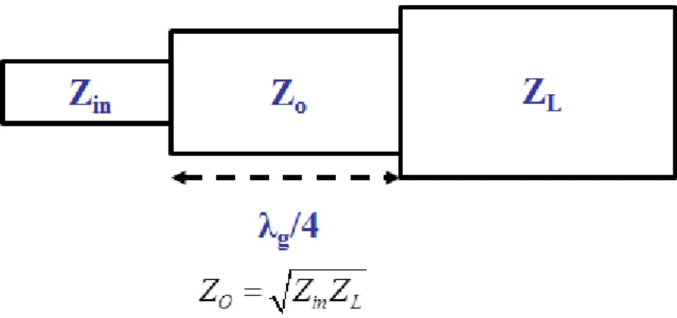
A 50 ohm SMA connector is using for connect the feed line to the coaxial cable. The feed line will be fed to the patch through a quarter-wave transformer matching network. A single microstrip patch antenna is consist of patch, quarter-wave transformer, and feed line as shown in Fig. 2.3.
The impedance of the quarter-wave transformer is given by Eq. (2.6), ……… (2.6)
where Zo is the transformer characteristic impedance and Zin is the
characteristic impedance of the input transmission line.
The patch antenna arrays have two types, first type is series array, and
l o l o Z -Z = Z +Z O in L
Z
Z Z
6
second type is parallel array. The parallel array has wider bandwidth, the impedance line design of four elements array is shown in Fig. 2.4, and the antenna array consists of a branching network of two-way power dividers. Quarter-wave transformers (70.7 ohm) are used to match the 100 ohm lines to the 50ohm lines, the impedance line are obtained using Eq. (2.6), where by
replacing Zin=50 ohm and ZL=100 ohm, the transformer characteristic
impedance is 70.7 ohm, and should avoid large impedance jumps, not to use single transformer from 50ohm to 250 ohm.
2.3 Antenna Element for Polarizations
In general, the antenna polarization decides by feed line to the element, the polarization of patch antenna is shown in Fig. 2.5. For Wi-Fi application, the outdoor AP usually use the vertical polarization, because the vertical polarization E-plane pattern is narrower, and the main beam focus on the front direction, the directivity will increase.
2.4 ECC
In MIMO antenna array system, Envelope Correlation Coefficient (ECC) shows the influence of different propagation paths of the RF signals that reach the antenna elements. In MIMO antenna system, the ECC is important. The approximated value of the ECC is from 0 to 1, quite perfect performance for MIMO applications is achieved when this parameter approximates to zero. And for only antenna, the ECC is must less than 0.3, if combine the device, it can be less than 0.5. The lower correlation, the higher diversity gain will be
7
achieved.
There are two methods to measurement the ECC, first is by far field pattern, it’s computation of correlation coefficient above requires radiation pattern of antennas and involves integral calculation, which is experimentally and numerically very time consuming. The method for calculating the ECC from far field pattern is shown in Eq. (2.7).
… (2.7) where is incident power spectrum for the different polarization, XPR is cross polarization ratio,
X and Y are antennas for different polarization.
To make this process easier, the second method is by S-parameters, the corresponding S-parameters that are provided by experimental procedure have been concentrated and used to the mathematical formula proposed. The method for calculating the ECC from S-parameters of the diversity antenna gain is shown in Eq. (2.8).
……… (2.8)
The ECC value for three ports is shown in Eq. (2.9).
……… (2.9)
2 * * 11 12 21 22 2 2 2 2 11 21 22 12 1 1 e S S S S S S S S
2 * * * 11 12 12 22 13 32 2 2 2 2 2 2 11 21 31 12 22 32 1 1 e S S S S S S S S S S S S
, P 8
Fig. 2.1. N elements antenna array
Fig. 2.2. Impedance matching circuit
9
Fig. 2.3. Patch antenna with quarter-wave transformer
10
(a) (b)
Fig. 2.5 Polarization of patch antenna (a) Vertical Polarization (b) Horizontal Polarization
Feed line
Feed line
11
Chapter 3
Antenna Array 2×1 for IEEE 802.11 b
3.1 Introduction
In this chapter, 2 by 1 antenna array for IEEE 802.11b have two parts. One part is vertical polarization antenna, the first is analysis the patch antenna's input impedance, using the slot between the element edge and transmission line for impedance matching
Second part is dual polarization for MIMO system, the dual polarization has more transmission line, that maybe cause mutual coupling effect antenna performance, and the distance between transmission line and edge is also consideration.
3.2 Single Polarization Simulation Model
The patch antenna radiation element size with operating frequency, substrate board thickness, and dielectric substrate are interrelated. The substrate is FR4 with thickness 0.08 cm, the relative permittivity is 4.2, and the loss tangent is 0.02. The height of the array to the ground is 0.25 cm. The size of ground and substrate is 16 cm in length and 7.1 cm in width. The simulation model by GEMS for 2 by 1 antenna array is shown in Fig. 3.1, the antenna radiation element is half-wavelength and square shape to design it. The length and width of radiation element are 4.75 cm, t is slot length, 0.3 cm as a unit to observe input impedance and antenna performance in different
12
length t, the comparison of S11 is shown in Fig. 3.2, from the result to know if
t is 0.6 cm will achieve the best impedance matching, Fig. 3.3 is shown the
Smith Chart that t is 0.6 cm, and the impedance most close to 50 ohm at 2.45 GHz.
3.3 Single Polarization Test Results
The Fig. 3.4 is shown the prototype of 2 by 1 antenna array, and feed on i-pax cable. The measurement environment of return loss is shown in Fig. 3.5,
S11 by simulation and measurement is shown in Fig. 3.6, the bandwidth of 10
dB is about 100 MHz (2400 MHz to 2500 MHz), which includes the IEEE 802.11b operating frequency.
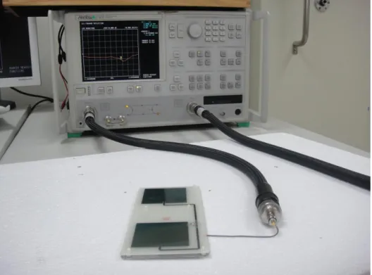
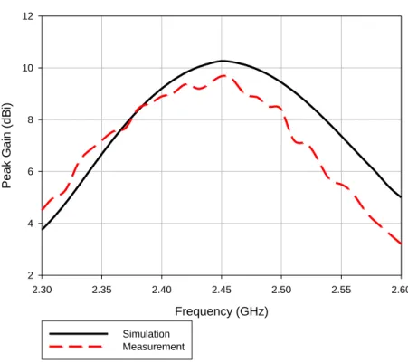
The measurement environment of power pattern is shown in Fig. 3.7. In this thesis, power pattern measured by SATIMO measurement system, SATIMO measurement system is near-filed to far-field system, it has 29 probes which composed of 15 low band (0.8 GHz to 6 GHz) probes and 14 high band (6 GHz to 18 GHz) probes, the general block diagram of SATIMO measurement system is shown in Fig. 3.8, the directivity by simulation and measurement is shown in Fig. 3.9, the directivity at 2.45 GHz is about 10.7 dBi, the peak gain by simulation and measurement is shown in Fig. 3.10, the peak gain at 2.45 GHz is about 9.5 dBi, the measurement result is small than simulation result, maybe due to the i-pax cable has larger loss, the efficiency by simulation and measurement is shown in Fig. 3.11, the efficiency at 2.45 GHz is about 81 %.
13
Channel 1 (2410 MHz), Channel 6 (2440 MHz) and Channel 11 (2460 MHz). The radiation pattern at 2410 MHz by simulation and measurement is shown in Fig. 3.12, the radiation pattern at 2440 MHz by simulation and measurement is shown in Fig. 3.13, the radiation pattern at 2460 MHz by simulation and measurement is shown in Fig. 3.14, the measurement result is similar to simulation result, and it have high directivity quality, the difference between co-pol and cross-pol 10 dB. The cross-pol has minor difference maybe due to improper hardware implementation or measurement.
The 3 dB beamwidth in E-plane is 31°, H-plane is 85°, that means the angle between the half-power (-3 dB) points of the main lobe. If the user is located inside 3 dB azimuth, it will be able to get the best signal. The 2 by 1 antenna array is for vertical polarization, so the E-plane beam pattern is narrow, and H-plane beam pattern is wider, it make directivity rise and suitable for outdoor AP.
3.4 Dual Polarization Simulation Model
This section design dual polarization antenna array for IEEE 802.11b, and it have multiple input and output, so it can applied for MIMO system.
The substrate is FR4 with thickness 0.08 cm, the relative permittivity is 4.2, and the loss tangent is 0.02. The height of the array to the ground is 0.25 cm. The size of ground and substrate is 16 cm in length and 7.1 cm in width. The simulation model by GEMS for 2 by 1 dual polarization antenna array is shown in Fig. 3.15. The length of radiation element is 4.75 cm, the feeding
14
radiation mismatch weighting spillover deielctric surfaceerror
total η η η η η η
η
must be on the center of transmission line to avoid the scan beam.
The transmission line and the edge of the board must have space, if the space is too close, it will reduce the antenna performance, and the width of transmission line is 1.5mm to impedance matching on i-pax.
3.5 Dual Polarization Test Results
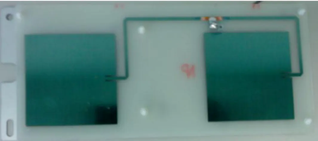
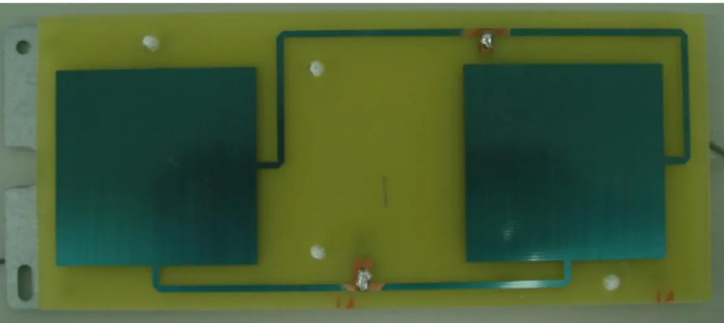
The Fig. 3.16 is shown the prototype of 2 by 1 dual polarization antenna
array. The S11 of vertical polarization and horizontal polarization is shown in
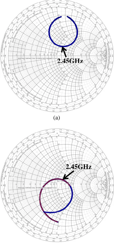
Fig. 3.17, the horizontal polarization bandwidth is wider than vertical polarization, both of polarizations have reach the operation bandwidth of IEEE802.11b, the flaws during the fabrication process may lead to the shift of the operating frequency of measurement result. The Smith chart of vertical polarization and horizontal polarization is shown in Fig. 3.18.
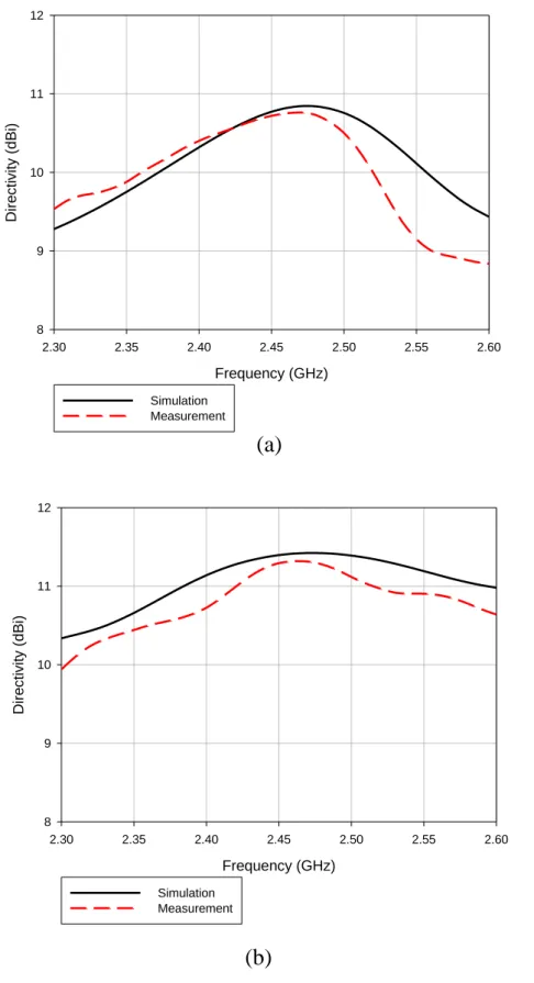
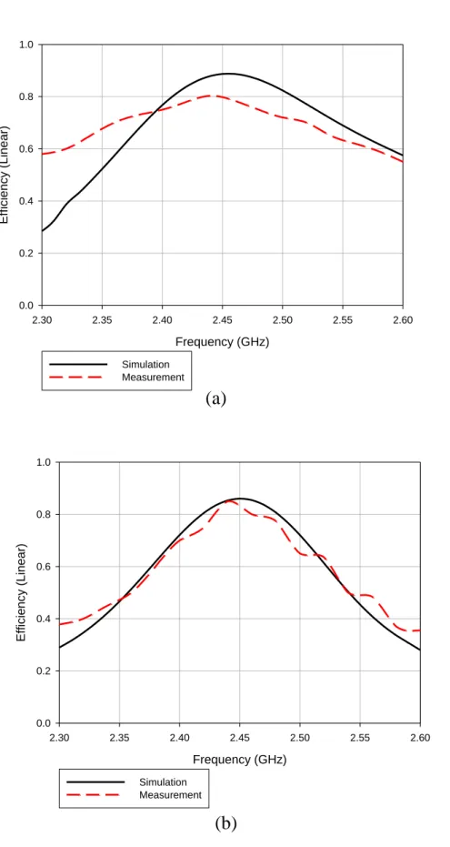
The directivity is shown in Fig. 3.19, the directivity of vertical polarization at 2.45 GHz is about 10.7 dBi, and horizontal polarization is about 11.3 dBi. The peak gain is shown in Fig. 3.20, the peak gain of vertical polarization at 2.45 GHz is about 9.3 dBi, and horizontal polarization is about 9.4 dBi. The efficiency is shown in Fig. 3.21, the efficiency of vertical polarization at 2.45 GHz is about 80 %, and the horizontal polarization is about 82 %. The relationship between gain and directivity is shown is Eq. (3.1).
……… (3.1) where
In order to increase the antenna gain, all these efficiencies should be as
Dir η
15
large as possible.
The vertical-pol radiation pattern at 2410 MHz is shown in Fig. 3.22, the horizontal-pol radiation pattern at 2410 MHz is shown in Fig. 3.23; the vertical-pol radiation pattern at 2440 MHz is shown in Fig. 3.24, the horizontal-pol radiation pattern at 2440 MHz is shown in Fig. 3.25; the vertical-pol radiation pattern at 2460 MHz is shown in Fig. 3.26, the horizontal-pol radiation pattern at 2460 MHz is shown in Fig. 3.27. The 2 by 1 antenna array is for vertical polarization, and the E-plane beam pattern is narrow, the difference between co-pol and cross-pol is about 20 dB, measurement result is similar to the simulation result. The 3 dB beamwidth in E-plane is 36°, H-plane is 74°for vertical polarization, and 3 dB beamwidth in E-plane is 70°, H-plane is 38° for horizontal polarization.
The ECC simulation result of 2 by 1 dual polarization antenna array by GEMS is shown in Fig. 3.28, the result of far field pattern and S-parameter are compared. The ECC result is less than 0.1, this observation indicates quite perfect behavior and performance of the MIMO antenna array system.
3.6 Summary
This chapter designed the 2 by 1 antenna array and all have good directivity quality, the mainbeam concentrate in the front direction, the lower back lobe can reduce back noise, so outdoor point to point Wi-Fi communication can be transmitted long distance and high throughput.
16 Frequency (GHz) 2.30 2.35 2.40 2.45 2.50 2.55 2.60 -30 -25 -20 -15 -10 -5 0 t = 0 t = 3 t = 6 t = 9 (Top View) (Side View)
Fig. 3.1 Simulation model of 2 by 1 antenna array
Fig. 3.2 Comparison of S11 in different slot length
4.75 t 9.45 3.01 0.25 Unit: cm Ground FR4 Feed Point 4.75 0.5
17
Fig. 3.3 Smith Chart (t = 0.6cm)
Fig. 3.4 Prototype of 2 by 1 antenna array
18
Fig. 3.5 Measurement environment of return loss
Fig. 3.6 S11 of 2 by 1 antenna array Frequency (GHz) 2.30 2.35 2.40 2.45 2.50 2.55 2.60 -30 -25 -20 -15 -10 -5 0 Simulation Measurement
19
20
Fig. 3.8 General block diagram of SATIMO measurement system
Fig. 3.9 Directivity of 2 by 1 antenna array
Frequency (GHz) 2.30 2.35 2.40 2.45 2.50 2.55 2.60 Direct iv it y (dB i) 6 7 8 9 10 11 12 Simulation Measurement
21
Fig. 3.10 Peak gain of 2 by 1 antenna array
Fig. 3.11 Efficiency of 2 by 1 antenna array
Frequency (GHz) 2.30 2.35 2.40 2.45 2.50 2.55 2.60 P eak Gai n (dB i) 2 4 6 8 10 12 Simulation Measurement Frequency (GHz) 2.30 2.35 2.40 2.45 2.50 2.55 2.60 E ff icie ncy (Linear) 0.0 0.2 0.4 0.6 0.8 1.0 Simulation Measurement
22 -30 -25 -20 -15 -10 -5 0 5 10 -30 -25 -20 -15 -10 -5 0 5 10 -30 -25 -20 -15 -10 -5 0 5 10 -30 -25 -20 -15 -10 -5 0 5 10 -90 -60 -30 0 30 60 90 120 150 180 210 240 (a) (b)
Fig. 3.12 Radiation pattern at 2410 MHz (a) E-plane (b) H-plane -30 -25 -20 -15 -10 -5 0 5 10 -30 -25 -20 -15 -10 -5 0 5 10 -30 -25 -20 -15 -10 -5 0 5 10 -30 -25 -20 -15 -10 -5 0 5 10 -90 -60 -30 0 30 60 90 120 150 180 210 240
23 -30 -25 -20 -15 -10 -5 0 5 10 -30 -25 -20 -15 -10 -5 0 5 10 -30 -25 -20 -15 -10 -5 0 5 10 -30 -25 -20 -15 -10 -5 0 5 10 -90 -60 -30 0 30 60 90 120 150 180 210 240 (a) (b)
Fig. 3.13 Radiation pattern at 2440 MHz (a) E-plane
(b) H-plane -30 -25 -20 -15 -10 -5 0 5 10 -30 -25 -20 -15 -10 -5 0 5 10 -30 -25 -20 -15 -10 -5 0 5 10 -30 -25 -20 -15 -10 -5 0 5 10 -90 -60 -30 0 30 60 90 120 150 180 210 240
24 -30 -25 -20 -15 -10 -5 0 5 10 -30 -25 -20 -15 -10 -5 0 5 10 -30 -25 -20 -15 -10 -5 0 5 10 -30 -25 -20 -15 -10 -5 0 5 10 -90 -60 -30 0 30 60 90 120 150 180 210 240 (a) (b)
Fig. 3.14 Radiation pattern at 2460 MHz (a) E-plane (b) H-plane -30 -25 -20 -15 -10 -5 0 5 10 -30 -25 -20 -15 -10 -5 0 5 10 -30 -25 -20 -15 -10 -5 0 5 10 -30 -25 -20 -15 -10 -5 0 5 10 -90 -60 -30 0 30 60 90 120 150 180 210 240
25
(Top View)
(Side View)
Fig. 3.15 Simulation model of 2 by 1 dual polarization antenna array
Fig. 3.16 Prototype of 2 by 1 dual polarization antenna array
0.5 0.49 4.75 4.75 9.45 9.45 3.01 VP HP 0.25 Unit: cm Ground FR4
26 Frequency (GHz) 2.30 2.35 2.40 2.45 2.50 2.55 2.60 -20 -18 -16 -14 -12 -10 -8 -6 -4 -2 0 Simulation Measurement (a) (b)
Fig. 3.17 S11 (a) Vertical polarization
(b) Horizontal polarization Frequency (GHz) 2.30 2.35 2.40 2.45 2.50 2.55 2.60 -18 -16 -14 -12 -10 -8 -6 -4 -2 0 Simulation Measurement
27
2.45GHz
(a)
(b)
Fig. 3.18 Smith chart (a) Vertical polarization (b) Horizontal polarization
28 Frequency (GHz) 2.30 2.35 2.40 2.45 2.50 2.55 2.60 Dire cti v it y (dB i) 8 9 10 11 12 Simulation Measurement (a) (b)
Fig. 3.19 Directivity (a) Vertical polarization (b) Horizontal polarization Frequency (GHz) 2.30 2.35 2.40 2.45 2.50 2.55 2.60 Dire cti v it y (dB i) 8 9 10 11 12 Simulation Measurement
29 Frequency (GHz) 2.30 2.35 2.40 2.45 2.50 2.55 2.60 P eak Gai n (dB i) 0 2 4 6 8 10 Simulation Measurement Frequency (GHz) 2.30 2.35 2.40 2.45 2.50 2.55 2.60 P eak Gai n (dB i) 2 4 6 8 10 12 Simulation Measurement (a) (b)
Fig. 3.20 Peak Gain (a) Vertical polarization (b) Horizontal polarization
30 Frequency (GHz) 2.30 2.35 2.40 2.45 2.50 2.55 2.60 E ff icie ncy (Linear) 0.0 0.2 0.4 0.6 0.8 1.0 Simulation Measurement Frequency (GHz) 2.30 2.35 2.40 2.45 2.50 2.55 2.60 E ff icie ncy (Linear) 0.0 0.2 0.4 0.6 0.8 1.0 Simulation Measurement (a) (b)
Fig. 3.21 Efficiency (a) Vertical polarization (b) Horizontal polarization
31 -30 -25 -20 -15 -10 -5 0 5 10 -30 -25 -20 -15 -10 -5 0 5 10 -30 -25 -20 -15 -10 -5 0 5 10 -30 -25 -20 -15 -10 -5 0 5 10 -90 -60 -30 0 30 60 90 120 150 180 210 240 (b) (a) (b)
Fig. 3.22 Vertical-pol radiation pattern at 2410 MHz (a) E-plane (b) H-plane -30 -25 -20 -15 -10 -5 0 5 10 -30 -25 -20 -15 -10 -5 0 5 10 -30 -25 -20 -15 -10 -5 0 5 10 -30 -25 -20 -15 -10 -5 0 5 10 -90 -60 -30 0 30 60 90 120 150 180 210 240
32 -30 -25 -20 -15 -10 -5 0 5 10 -30 -25 -20 -15 -10 -5 0 5 10 -30 -25 -20 -15 -10 -5 0 5 10 -30 -25 -20 -15 -10 -5 0 5 10 -90 -60 -30 0 30 60 90 120 150 180 210 240 -30 -25 -20 -15 -10 -5 0 5 10 -30 -25 -20 -15 -10 -5 0 5 10 -30 -25 -20 -15 -10 -5 0 5 10 -30 -25 -20 -15 -10 -5 0 5 10 -90 -60 -30 0 30 60 90 120 150 180 210 240 (a) (b)
Fig. 3.23 Horizontal-pol radiation pattern at 2410 MHz (a) E-plane (b) H-plane
33 -30 -25 -20 -15 -10 -5 0 5 10 -30 -25 -20 -15 -10 -5 0 5 10 -30 -25 -20 -15 -10 -5 0 5 10 -30 -25 -20 -15 -10 -5 0 5 10 -90 -60 -30 0 30 60 90 120 150 180 210 240 -30 -25 -20 -15 -10 -5 0 5 10 -30 -25 -20 -15 -10 -5 0 5 10 -30 -25 -20 -15 -10 -5 0 5 10 -30 -25 -20 -15 -10 -5 0 5 10 -90 -60 -30 0 30 60 90 120 150 180 210 240 (a) (b)
Fig. 3.24 Vertical-pol radiation pattern at 2440 MHz (a) E-plane (b) H-plane
34 -30 -25 -20 -15 -10 -5 0 5 10 -30 -25 -20 -15 -10 -5 0 5 10 -30 -25 -20 -15 -10 -5 0 5 10 -30 -25 -20 -15 -10 -5 0 5 10 -90 -60 -30 0 30 60 90 120 150 180 210 240 (a) (b)
Fig. 3.25 Horizontal-pol radiation pattern at 2440 MHz (a) E-plane (b) H-plane -30 -25 -20 -15 -10 -5 0 5 10 -30 -25 -20 -15 -10 -5 0 5 10 -30 -25 -20 -15 -10 -5 0 5 10 -30 -25 -20 -15 -10 -5 0 5 10 -90 -60 -30 0 30 60 90 120 150 180 210 240
35 -30 -25 -20 -15 -10 -5 0 5 10 -30 -25 -20 -15 -10 -5 0 5 10 -30 -25 -20 -15 -10 -5 0 5 10 -30 -25 -20 -15 -10 -5 0 5 10 -90 -60 -30 0 30 60 90 120 150 180 210 240 -30 -25 -20 -15 -10 -5 0 5 10 -30 -25 -20 -15 -10 -5 0 5 10 -30 -25 -20 -15 -10 -5 0 5 10 -30 -25 -20 -15 -10 -5 0 5 10 -90 -60 -30 0 30 60 90 120 150 180 210 240 (a) (b)
Fig. 3.26 Vertical-pol radiation pattern at 2460 MHz (a) E-plane (b) H-plane
36 -30 -25 -20 -15 -10 -5 0 5 10 -30 -25 -20 -15 -10 -5 0 5 10 -30 -25 -20 -15 -10 -5 0 5 10 -30 -25 -20 -15 -10 -5 0 5 10 -90 -60 -30 0 30 60 90 120 150 180 210 240 (a) (b)
Fig. 3.27 Horizontal-pol radiation pattern at 2460 MHz (a) E-plane (b) H-plane -30 -25 -20 -15 -10 -5 0 5 10 -30 -25 -20 -15 -10 -5 0 5 10 -30 -25 -20 -15 -10 -5 0 5 10 -30 -25 -20 -15 -10 -5 0 5 10 -90 -60 -30 0 30 60 90 120 150 180 210 240
37
Fig. 3.28 ECC simulation result of 2 by 1 antenna array
Frequency (GHz) 2.30 2.35 2.40 2.45 2.50 2.55 2.60 E CC 0.00 0.02 0.04 0.06 0.08 0.10 Far-Field pattern S-parameters
38
Chapter 4
Antenna Array 4×1 for IEEE 802.11 a
4.1 Introduction
This chapter presents 4 by 1 antenna array for IEEE802.11a and design dual polarization antennas. The bandwidth requirement is for IEEE802.11a Wi-Fi is from 5.2 GHz to 5.8 GHz. For lower directivity antenna, it will be easier to obtain the 11 % bandwidth (5.2 GHz~5.8 GHz) for IEEE802.11a, but for high directivity antenna is difficult.
Since the operating frequency is 5 GHz, the element size is according to half-wavelength to design, the element size is smaller than 2.45 GHz element. Therefore, it can be designed four elements in the same substrate board, and the gain can be higher than two arrays antenna.
For four antenna array, it needs to design power divider for impedance matching, the designed of power divider to introduction in the next section.
4.2 Single Polarization Simulation Model
The simulation model by GEMS for 4 by 1 antenna array is shown in Fig. 4.1, the substrate is FR4 with thickness 0.04 cm, the relative permittivity is 4.2, and the loss tangent is 0.02. The height of the array to the ground is 0.25 cm. The size of ground and substrate is 16 cm in length and 7.1 cm in width. The antenna radiation element is half-wavelength and square shape to design
39
it. The length and width of radiation element are 1.9 cm.
The antenna array consists of two-way power dividers, the impedance for the 4 by 1 antenna array is shown in Fig. 4.2, calculation for impedance is also similar to a single patch calculation by Eq. (2.6), the width of 50 ohm transmission line is 1.5 mm, which can not close to element to reduce mutual coupling. The width of 35.4 ohm transmission line is 2.6 mm, the width of 70.7 ohm transmission line is 0.8 mm, and the feed line is 50 ohm for impedance matching on i-pax cable.
4.3 Single Polarization Test Results
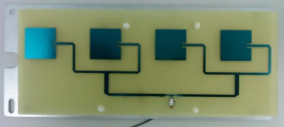
The prototype of 4 by 1 single polarization antenna array is shown in Fig
4.3. S11 by simulation and measurement is shown in Fig. 4.3, the IEEE
802.11a band is wider, it is about 1 GHz bandwidth, but patch antenna bandwidth is narrow, that is disadvantage, from the result, from 5.3 GHz to 5.8 GHz almost 10 dB, but the impedance is worse in low frequency (5.2GHz), the Smith Chart is shown is Fig. 4.5.
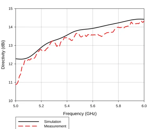
The directivity by simulation and measurement is shown in Fig. 4.6, the directivity is about 13 to 14 dBi, the peak gain by simulation and measurement is shown in Fig. 4.7, the peak gain is about 8 to 10 dBi, the low band is low, due to the impedance worse, the efficiency by simulation and measurement is shown in Fig. 4.8. The more array element and gain will raise, the antenna array gain estimate as shown in Eq. (4.1), and the substrate thickness, material, and other loss will affect antenna gain.
40
(dBi) ……… (4.1) where N is number of elements,
ηis efficiency,
5 is element gain for a typical patch.
The radiation pattern at 5200 MHz by simulation and measurement is shown in Fig. 4.9, the radiation pattern at 5500 MHz by simulation and measurement is shown in Fig. 4.10, the radiation pattern at 5800 MHz by simulation and measurement is shown in Fig. 4.11. Due to the four array, the radiation pattern has larger sidelobe, the difference between co-pol and cross-pol almost 15 dB. The 3 dB beamwidth in E-plane is 19°, H-plane is 82 °.
4.4 Dual Polarization Simulation Model
The simulation model by GEMS for 4 by 1 dual polarization antenna array is shown in Fig. 4.12, the substrate is FR4 with thickness 0.04 cm, the relative permittivity is 4.2, and the loss tangent is 0.02. The height of the array to the ground is 0.25 cm. The size of ground and substrate is 16 cm in length and 7.1 cm in width.
The impedance is same with single polarization, the transmission line can not close to element to avoid reduce antenna gain. The feeding on the center of transmission line avoid the beam pattern to scan.
10
10log
5
41
4.5 Dual Polarization Test Results
Fig. 4.13 is shown the prototype of 4 by 1 dual polarization antenna array. The S11 of vertical polarization and horizontal polarization is shown in Fig.
4.14, both of polarizations of bandwidth are narrow, and the impedance is bad in low band. The Smith chart of vertical polarization and horizontal polarization is shown in Fig. 4.15.
The directivity is shown in Fig. 4.16, the directivity of vertical polarization is about 14 dBi, and horizontal polarization is about 15 dBi. The peak gain is shown in Fig. 4.17, the peak gain of vertical polarization is about 11 dBi, and horizontal polarization is about 12 dBi. The efficiency is shown in Fig. 4.18, the efficiency of vertical and horizontal polarization is lower in low band.
The vertical-pol radiation pattern at 5200 MHz is shown in Fig. 4.19, the horizontal-pol radiation pattern at 5200 MHz is shown in Fig. 4.20; the vertical-pol radiation pattern at 5500 MHz is shown in Fig. 4.21, the horizontal-pol radiation pattern at 5500 MHz is shown in Fig. 4.22; the vertical-pol radiation pattern at 5800 MHz is shown in Fig. 4.23, the horizontal-pol radiation pattern at 5800 MHz is shown in Fig. 4.24. The difference between co-pol and cross-pol is about 15 dB. 3 dB beamwidth in E-plane is 15°, H-plane is 68°for vertical polarization, and 3 dB beamwidth in E-plane is 48°, H-plane is 19° for horizontal polarization.
42
GEMS is shown in Fig. 4.25. The ECC result is less than 0.1 for frequency from 5 GHz to 6 GHz, in low band the ECC value is higher than high band.
4.6 Summary
This chapter design 4 by 1 antenna array, dual polarization antenna gain is about 10 dBi. If the power divider can design well, it cans radiate larger energy by four element array. Because it has four array elements and radiation patters have larger sidelobe.
As the IEEE 802.11a operating frequency is wider, and the patch antenna bandwidth is narrow, next chapter will design another transmission line to increase bandwidth.
43
(Top View)
(Side View)
Fig. 4.1 Simulation model of 4 by 1 antenna array
Fig. 4.2 Impedance for 4 by 1 antenna array
1.9 1.58 1.23 0.75 1.9 1.35 3.58 3.525 0.69 50ohm 50ohm 50ohm 35.4ohm 70.7ohm 0.25 Unit: cm Ground FR4 Feed Point
44
Fig. 4.3 Prototype of 4 by 1 antenna array
Fig. 4.4 S11 of 4 by 1 antenna array Frequency (GHz) 5.0 5.2 5.4 5.6 5.8 6.0 -30 -25 -20 -15 -10 -5 0 Simulation Measurement
45
Fig. 4.5 Smith Chart (5 GHz to 6 GHz)
Fig. 4.6 Directivity of 4 by 1 antenna array
Frequency (GHz) 5.0 5.2 5.4 5.6 5.8 6.0 Direct iv it y (dB i) 10 11 12 13 14 15 Simulation Measurement
46
Fig. 4.7 Peak Gain of 4 by 1 antenna array
Fig. 4.8 Efficiency of 4 by 1 antenna array
Frequency (GHz) 5.0 5.2 5.4 5.6 5.8 6.0 P eak Gai n (dB i) 0 2 4 6 8 10 12 14 16 Simulation Measurement Frequency (GHz) 5.0 5.2 5.4 5.6 5.8 6.0 E ff icie ncy (Linear) 0.0 0.2 0.4 0.6 0.8 1.0 Simulation Measurement
47 -30 -25 -20 -15 -10 -5 0 5 10 -30 -25 -20 -15 -10 -5 0 5 10 -30 -25 -20 -15 -10 -5 0 5 10 -30 -25 -20 -15 -10 -5 0 5 10 -90 -60 -30 0 30 60 90 120 150 180 210 240 -30 -25 -20 -15 -10 -5 0 5 10 -30 -25 -20 -15 -10 -5 0 5 10 -30 -25 -20 -15 -10 -5 0 5 10 -30 -25 -20 -15 -10 -5 0 5 10 -90 -60 -30 0 30 60 90 120 150 180 210 240 (a) (b)
Fig. 4.9 Radiation pattern at 5200 MHz (a) E-plane (b) H-plane
48 -30 -25 -20 -15 -10 -5 0 5 10 -30 -25 -20 -15 -10 -5 0 5 10 -30 -25 -20 -15 -10 -5 0 5 10 -30 -25 -20 -15 -10 -5 0 5 10 -90 -60 -30 0 30 60 90 120 150 180 210 240 (a) (b)
Fig. 4.10 Radiation pattern at 5500 MHz (a) E-plane (b) H-plane -30 -25 -20 -15 -10 -5 0 5 10 -30 -25 -20 -15 -10 -5 0 5 10 -30 -25 -20 -15 -10 -5 0 5 10 -30 -25 -20 -15 -10 -5 0 5 10 -90 -60 -30 0 30 60 90 120 150 180 210 240
49 -25 -20 -15 -10 -5 0 5 10 15 -25 -20 -15 -10 -5 0 5 10 15 -25 -20 -15 -10 -5 0 5 10 15 -25 -20 -15 -10 -5 0 5 10 15 -90 -60 -30 0 30 60 90 120 150 180 210 240 (a) (a) (b)
Fig. 4.11 Radiation pattern at 5800 MHz (a) E-plane (b) H-plane -25 -20 -15 -10 -5 0 5 10 15 -25 -20 -15 -10 -5 0 5 10 15 -25 -20 -15 -10 -5 0 5 10 15 -25 -20 -15 -10 -5 0 5 10 15 -90 -60 -30 0 30 60 90 120 150 180 210 240
50
(Top View)
(Side View)
Fig. 4.12 Simulation model of 4 by 1 dual polarization antenna array
Fig. 4.13 Prototype of 4 by 1 dual polarization antenna array
VP
HP
1.9 1.9 0.875 1.23 1.2 3.85 3.525 0.75 0.69 0.25 Unit: cm Ground FR451 Frequency (GHz) 5.0 5.2 5.4 5.6 5.8 6.0 Y Data -20 -15 -10 -5 0 Simulation Measurement Frequency (GHz) 5.0 5.2 5.4 5.6 5.8 6.0 Y Data -20 -15 -10 -5 0 Simulation Measurement (a) (b)
Fig. 4.14 S11 (a) Vertical polarization
52
(a)
(b)
Fig. 4.15 Smith chart (5 GHz to 6 GHz) (a) Vertical polarization (b) Horizontal polarization
53 Frequency (GHz) 5.0 5.2 5.4 5.6 5.8 6.0 Direct iv it y (dB i) 10 11 12 13 14 15 16 Simulation Measurement Frequency (GHz) 5.0 5.2 5.4 5.6 5.8 6.0 Direct iv it y (dB i) 10 11 12 13 14 15 16 Simulation Measurement (a) (b)
Fig. 4.16 Directivity (a) Vertical polarization (b) Horizontal polarization
54 Frequency (GHz) 5.0 5.2 5.4 5.6 5.8 6.0 P eak Gai n (dB i) 0 2 4 6 8 10 12 14 16 Simulation Measurement Frequency (GHz) 5.0 5.2 5.4 5.6 5.8 6.0 P eak Gai n (dB i) 0 2 4 6 8 10 12 14 16 Simulation Measurement (a) (b)
Fig. 4.17 Peak gain (a) Vertical polarization (b) Horizontal polarization
55 Frequency (GHz) 5.0 5.2 5.4 5.6 5.8 6.0 E ff icie ncy (Linear) 0.0 0.2 0.4 0.6 0.8 1.0 Simulation Measurement Frequency (GHz) 5.0 5.2 5.4 5.6 5.8 6.0 E ff icie ncy (Linear) 0.0 0.2 0.4 0.6 0.8 1.0 Simulation Measurement (a) (b)
Fig. 4.18 Efficiency (a) Vertical polarization (b) Horizontal polarization
56 -30 -25 -20 -15 -10 -5 0 5 10 -30 -25 -20 -15 -10 -5 0 5 10 -30 -25 -20 -15 -10 -5 0 5 10 -30 -25 -20 -15 -10 -5 0 5 10 -90 -60 -30 0 30 60 90 120 150 180 210 240 (a) (b)
Fig. 4.19 Vertical-pol radiation pattern at 5200 MHz (a) E-plane (b) H-plane -30 -25 -20 -15 -10 -5 0 5 10 -30 -25 -20 -15 -10 -5 0 5 10 -30 -25 -20 -15 -10 -5 0 5 10 -30 -25 -20 -15 -10 -5 0 5 10 -90 -60 -30 0 30 60 90 120 150 180 210 240
57 -30 -25 -20 -15 -10 -5 0 5 10 -30 -25 -20 -15 -10 -5 0 5 10 -30 -25 -20 -15 -10 -5 0 5 10 -30 -25 -20 -15 -10 -5 0 5 10 -90 -60 -30 0 30 60 90 120 150 180 210 240 (a) (a) (b)
Fig. 4.20 Horizontal-pol pattern at 5200 MHz (a) E-plane (b) H-plane -30 -25 -20 -15 -10 -5 0 5 10 -30 -25 -20 -15 -10 -5 0 5 10 -30 -25 -20 -15 -10 -5 0 5 10 -30 -25 -20 -15 -10 -5 0 5 10 -90 -60 -30 0 30 60 90 120 150 180 210 240
58 -30 -25 -20 -15 -10 -5 0 5 10 -30 -25 -20 -15 -10 -5 0 5 10 -30 -25 -20 -15 -10 -5 0 5 10 -30 -25 -20 -15 -10 -5 0 5 10 -90 -60 -30 0 30 60 90 120 150 180 210 240 (a) (a) (b)
Fig. 4.21 Vertical-pol radiation pattern at 5500 MHz (a) E-plane (b) H-plane -30 -25 -20 -15 -10 -5 0 5 10 -30 -25 -20 -15 -10 -5 0 5 10 -30 -25 -20 -15 -10 -5 0 5 10 -30 -25 -20 -15 -10 -5 0 5 10 -90 -60 -30 0 30 60 90 120 150 180 210 240
59 -25 -20 -15 -10 -5 0 5 10 15 -25 -20 -15 -10 -5 0 5 10 15 -25 -20 -15 -10 -5 0 5 10 15 -25 -20 -15 -10 -5 0 5 10 15 -90 -60 -30 0 30 60 90 120 150 180 210 240 (a) (a) (b)
Fig. 4.22 Horizontal-pol radiation pattern at 5500 MHz (a) E-plane (b) H-plane -50 -40 -30 -20 -10 0 10 -50 -40 -30 -20 -10 0 10 -50 -40 -30 -20 -10 0 10 -50 -40 -30 -20 -10 0 10 -90 -60 -30 0 30 60 90 120 150 180 210 240
60 -25 -20 -15 -10 -5 0 5 10 15 -25 -20 -15 -10 -5 0 5 10 15 -25 -20 -15 -10 -5 0 5 10 15 -25 -20 -15 -10 -5 0 5 10 15 -90 -60 -30 0 30 60 90 120 150 180 210 240 (a) (a) (b)
Fig. 4.23 Vertical-pol radiation pattern at 5800 MHz (a) E-plane (b) H-plane -25 -20 -15 -10 -5 0 5 10 15 -25 -20 -15 -10 -5 0 5 10 15 -25 -20 -15 -10 -5 0 5 10 15 -25 -20 -15 -10 -5 0 5 10 15 -90 -60 -30 0 30 60 90 120 150 180 210 240
61 -25 -20 -15 -10 -5 0 5 10 15 -25 -20 -15 -10 -5 0 5 10 15 -25 -20 -15 -10 -5 0 5 10 15 -25 -20 -15 -10 -5 0 5 10 15 -90 -60 -30 0 30 60 90 120 150 180 210 240 (a) (b)
Fig. 4.24 Horizontal-pol radiation pattern at 5800 MHz (a) E-plane (b) H-plane -50 -40 -30 -20 -10 0 10 -50 -40 -30 -20 -10 0 10 -50 -40 -30 -20 -10 0 10 -50 -40 -30 -20 -10 0 10 -90 -60 -30 0 30 60 90 120 150 180 210 240
62
Fig. 4.25 ECC simulation result of 4 by 1 antenna array
Frequency (GHz) 5.0 5.2 5.4 5.6 5.8 6.0 E CC 0.00 0.02 0.04 0.06 0.08 0.10 Far-Field pattern S-parameters
63
Chapter 5
Antenna Array 4×2 for IEEE 802.11 a
5.1 Introduction
This chapter presents the 4 by 2 antenna array for IEEE802.11a. In last chapter, the 4 by 1 antenna array bandwidth is narrow, so in this chapter, the transmission line is designed by taper line for impedance matching to increase bandwidth.
Usually, if antenna elements are increased, the higher the directivity of the antenna array will be high. Unfortunately, if the antenna size is limited, the directivity will be limited even if the antenna elements are increased, and the complex transmission line will reduce the antenna performance.
Grating lobes are typically undesirable in many communication systems, and it will limit the bandwidth of antenna array. If the spacing between antenna elements is more than half wavelength, the grating lobes usually occur, and the grating lobes usually occur in high frequency of antenna array.
5.2 Single Polarization Simulation Model
The simulation model by GEMS for 4 by 2 antenna array is shown in Fig. 5.1, the substrate is FR4 with thickness 0.04 cm, the relative permittivity is 4.2, and the loss tangent is 0.02. The height of the array to the ground is 0.25 cm. The size of ground and substrate is 16 cm in length and 7.1 cm in width.
64
The impedance in the 4 by 2 antenna array is shown in Fig. 5.2, the 200 ohm to 100 ohm is designed by taper line, and it can increase bandwidth.
5.3 Single Polarization Test Results
The prototype of 4 by 2 single polarization antenna array is shown in Fig.
5.3. S11 by simulation and measurement is shown in Fig. 5.4, the bandwidth is
wider than last chapter 4 by 1 antenna array. The Smith Chart as shown is Fig. 5.5.
The directivity by simulation and measurement is shown in Fig. 5.6, the directivity is about 15 to 16 dBi, the peak gain by simulation and measurement is shown in Fig. 5.7, the peak gain is about 12 to 14 dBi, the peak gain in high band is lower, the efficiency by simulation and measurement is shown in Fig. 5.8, the efficiency is about 60 % to 70%.
The radiation pattern at 5200 MHz by simulation and measurement is shown in Fig. 5.9, the radiation pattern at 5500 MHz by simulation and measurement is shown in Fig. 5.10, the radiation pattern at 5800 MHz by simulation and measurement is shown in Fig. 5.11. The difference between co-pol and cross-pol almost 15 dB. The 3 dB beamwidth in E-plane is 19°, H-plane is 45°. Although the feed in is in H-plane with limit size, the H-plane pattern is a little titled.
65
5.4 Dual Polarization Simulation Model
The simulation model by GEMS for 4 by o1 dual polarization antenna array is shown in Fig. 5.12, the substrate is FR4 with thickness 0.04 cm, the relative permittivity is 4.2, and the loss tangent is 0.02. The height of the array to the ground is 0.25 cm. The size of ground and substrate is 20 cm in length and 9 cm in width.
The impedance is same with single polarization, the 200 ohm to 100 ohm is designed by taper line. The each transmission line can not too close to avoid mutual coupling.
5.5 Dual Polarization Test Results
The Fig. 5.13 is shown the prototype of 4 by 2 dual polarization antenna
array. The S11 of vertical polarization and horizontal polarization as shown in
Fig. 5.14, S11 of vertical polarization from 5 GHz to 6 GHz achieve 10 dB,
and horizontal polarization is less in low band. The Smith chart of vertical polarization and horizontal polarization is shown in Fig. 5.15.
The directivity is shown in Fig. 5.16, the directivity of vertical polarization and horizontal polarization is about 14 to 15 dBi. The peak gain is shown in Fig. 5.17, the peak gain of vertical polarization and horizontal polarization is about 12 to 13.5 dBi. The efficiency is shown in Fig. 5.18, the efficiency of vertical polarization and horizontal polarization is 60 % to 70 %, which maybe due to the inaccuracy of manufacture.
66
The vertical polarization radiation pattern at 5200 MHz is shown in Fig. 5.19, the horizontal-pol radiation pattern at 5200 MHz is shown in Fig. 5.20; the vertical-pol radiation pattern at 5500 MHz is shown in Fig. 5.21, the horizontal-pol radiation pattern at 5500 MHz is shown in Fig. 5.22; the vertical-pol radiation pattern at 5800 MHz is shown in Fig. 5.23, the horizontal-pol radiation pattern at 5800 MHz is shown in Fig. 5.24. The difference between co-pol and cross-pol is about 20 dB. It is eight antenna elements, so the radiation patterns have higher directivity quality and sidelobe. The 3 dB beamwidth in E-plane is 14°, H-plane is 45° for vertical polarization, and 3 dB beamwidth in E-plane is 51 °, H-plane is 16 ° for horizontal polarization.
The radiation pattern at 5800 MHz have apparent grating lobe, because antenna elements is more than half wavelength, the antenna performance also reduce.
The ECC simulation result of 4 by 2 dual polarization antenna array by GEMS is shown in Fig. 5.25. The ECC result is less than 0.1 for frequency from 5 GHz to 6 GHz, and more antenna element the ECC will be worse.
5.6 Summary
This chapter presents the 4 by 2 dual and single polarization antenna array for IEEE802.11a. The gain of eight array elements is higher than four array elements, and using tapered line to increase bandwidth. Usually, the more the antenna elements, the higher the directivity of the antenna array will be, but
67
the complex transmission line or elements reduce energy.
The directivity of dual polarization is higher than single polarization, the reason is the substrate size of dual polarization is larger, it has larger space to reduce mutual coupling, but the grating lobe is occurred. So how to choose is also need to consider.
68
(Top View)
(Side View)
Fig. 5.1 Simulation model of 4 by 2 antenna array
Fig. 5.2 Impedance for 4 by 2 antenna array
2.15 2.15 2.77 2.86 0.68 0.5 3.65 3.025 1.7 0.2 50ohm 50ohm 100ohm 200ohm 25ohm 70.7ohm 0.25 Unit: cm Ground FR4 Feed Point
69
Fig. 5.3 Prototype of 4 by 2 antenna array
Fig. 5.4 S11 of 4 by 2 antenna array Frequency (GHz) 5.0 5.2 5.4 5.6 5.8 6.0 -30 -25 -20 -15 -10 -5 0 Simulation Measurement
70
Fig. 5.5 Smith Chart (5 GHz to 6 GHz)
Fig. 5.6 Directivity of 4 by 2 antenna array
Frequency (GHz) 5.0 5.2 5.4 5.6 5.8 6.0 Dir ectiv it y (dBi) 10 11 12 13 14 15 16 17 Simulation Measurement
71
Fig. 5.7 Peak Gain of 4 by 2 antenna array
Fig. 5.8 Efficiency of 4 by 2 antenna array
Frequency (GHz) 5.0 5.2 5.4 5.6 5.8 6.0 Pea k Gain (dBi) 4 6 8 10 12 14 16 Simulation Measurement Frequency (GHz) 5.0 5.2 5.4 5.6 5.8 6.0 E ff icie ncy (Linear) 0.0 0.2 0.4 0.6 0.8 1.0 Simulation Measurement
72 -25 -20 -15 -10 -5 0 5 10 15 -25 -20 -15 -10 -5 0 5 10 15 -25 -20 -15 -10 -5 0 5 10 15 -25 -20 -15 -10 -5 0 5 10 15 -90 -60 -30 0 30 60 90 120 150 180 210 240 (a) (a) (b)
Fig. 5.9 Radiation pattern at 5200 MHz (a) E-plane (b) H-plane -25 -20 -15 -10 -5 0 5 10 15 -25 -20 -15 -10 -5 0 5 10 15 -25 -20 -15 -10 -5 0 5 10 15 -25 -20 -15 -10 -5 0 5 10 15 -90 -60 -30 0 30 60 90 120 150 180 210 240
73 -25 -20 -15 -10 -5 0 5 10 15 -25 -20 -15 -10 -5 0 5 10 15 -25 -20 -15 -10 -5 0 5 10 15 -25 -20 -15 -10 -5 0 5 10 15 -90 -60 -30 0 30 60 90 120 150 180 210 240 (a) (a) (b)
Fig. 5.10 Radiation pattern at 5500 MHz (a) E-plane (b) H-plane -25 -20 -15 -10 -5 0 5 10 15 -25 -20 -15 -10 -5 0 5 10 15 -25 -20 -15 -10 -5 0 5 10 15 -25 -20 -15 -10 -5 0 5 10 15 -90 -60 -30 0 30 60 90 120 150 180 210 240
74 -25 -20 -15 -10 -5 0 5 10 15 -25 -20 -15 -10 -5 0 5 10 15 -25 -20 -15 -10 -5 0 5 10 15 -25 -20 -15 -10 -5 0 5 10 15 -90 -60 -30 0 30 60 90 120 150 180 210 240 (a) (a) (b)
Fig. 5.11 Radiation pattern at 5800 MHz (a) E-plane (b) H-plane -25 -20 -15 -10 -5 0 5 10 15 -25 -20 -15 -10 -5 0 5 10 15 -25 -20 -15 -10 -5 0 5 10 15 -25 -20 -15 -10 -5 0 5 10 15 -90 -60 -30 0 30 60 90 120 150 180 210 240
75
(Top View)
(Side View)
Fig. 5.12 Simulation model of 4 by 2 dual polarization antenna array
Fig. 5.13 Prototype of 4 by 2 dual polarization antenna array
VP HP 2.15 3.37 0.5 3.42 2.2 2.86 0.68 2.15 0.85 4.2 4.175 1.7 1.52 0.25 Unit: cm Ground FR4
76 Frequency (GHz) 5.0 5.2 5.4 5.6 5.8 6.0 -25 -20 -15 -10 -5 0 Simulation Measurement Frequency (GHz) 5.0 5.2 5.4 5.6 5.8 6.0 -35 -30 -25 -20 -15 -10 -5 0 Simulation Measurement (a) (b)
Fig. 5.14 S11 (a) Vertical polarization