Estimation of 2-D Noisy Fractional Brownian Motion and Its Applications Using Wavelets

Estimation of 2-D Noisy Fractional Brownian Motion

and its Applications Using Wavelets

Jen-Chang Liu, Wen-Liang Hwang, and Ming-Syan Chen, Senior Member, IEEE

Abstract—The two-dimensional (2-D) fractional Brownian mo-tion (fBm) model is useful in describing natural scenes and tex-tures. Most fractal estimation algorithms for 2-D isotropic fBm im-ages are simple extensions of the one-dimensional (1-D) fBm esti-mation method. This method does not perform well when the image size is small (say, 32 32). We propose a new algorithm that esti-mates the fractal parameter from the decay of the variance of the wavelet coefficients across scales. Our method places no restric-tion on the wavelets. Also, it provides a robust parameter estima-tion for small noisy fractal images. For image denoising, a Wiener filter is constructed by our algorithm using the estimated param-eters and is then applied to the noisy wavelet coefficients at each scale. We show that the averaged power spectrum of the denoised image is isotropic and is a nearly1 process. The performance of our algorithm is shown by numerical simulation for both the fractal parameter and the image estimation. Applications on coast-line detection and texture segmentation in noisy environment are also demonstrated.

Index Terms—Denoising, fractional Brownian motion, texture analysis, wavelet transform.

I. INTRODUCTION

F

where is the scaling exponent, . Other types of 2-D fBm, such as the multifractal rough surface [25] and the ex-tended self-similar model [10], also exhibit features controlled by the scaling exponent . Many natural phenomena are found to have spectrums. Thus, an fBm provides good mathe-matical modeling of these phenomena. Moreover, the self-sim-ilar property, which means that the statistical measure is in-variant to the change of scales, makes fBm very useful in de-scribing natural scenes and textures. The scaling exponent has

Manuscript received October 2, 1998; revised January 11, 2000. W.-L. Hwang and J.-C. Liu were supported by NSC Project 88-2213-E-001-028. M.-S. Chen was supported in part by the Ministry of Education under Project 89-E-FA06-2-4-7. The associate editor coordinating the review of this manuscript and approving it for publication was Prof. Kannan Ramchandran.

J.-C. Liu is with the Department of Electrical Engineering, National Taiwan University, Taipei, Taiwan, R.O.C. He is also with the Institute of Information Science, Academia Sinica, Taiwan, R.O.C.

W.-L. Hwang is with the Institute of Information Science, Academia Sinica, Taiwan, R.O.C.

M.-S. Chen is with the Department of Electrical Engineering, National Taiwan University, Taipei, Taiwan, R.O.C.

Publisher Item Identifier S 1057-7149(00)06141-8.

also been shown to be related to the fractal dimension and sur-face roughness [16]. Many research works have focused on the generation of fBm [11], [20] and estimation of the fractal pa-rameter (scaling exponent) [2], [8], [12], [21]. Among them, the wavelet approach was adopted naturally because the statis-tical self-similarity properties of an fBm can be described based on the scaling properties of wavelet transforms. Most of the previous wavelet-based results have depended heavily on the orthogonality and vanishing moment of the wavelet function. They used the approximation that the orthogonal wavelet coef-ficients are almost white processes. This approximation works only if orthogonal wavelets with high vanishing moment are used. The performance will severely degrade if nonorthogonal wavelets are used. It was shown in [7] that the orthogonality of a wavelet can be discarded if the fractal parameter is esti-mated from the autocorrelation of the wavelet transform of an fBm. In spite of the comparative performance of the fBm esti-mation and denoising methods with the results obtained using orthogonal wavelet transform, the approach in [7] allows fractal estimation and other applications, such as edge detection and instantaneous frequency analysis, both of which are captured nicely by nonorthogonal wavelet transforms, to be done with one wavelet transform analysis [3], [13], [14].

In this paper, we will extend the proposed methods in [7] to an isotropic 2-D noisy fBm image. The extension is not straightforward. Although one can obtain the fractal parameter of an isotropic fBm by averaging the estimated fractal param-eters from several directions using the one-dimensional (1-D) fractal parameter estimation algorithm [2], [9], [12], [22], this approach does not work well in practice. Note that when the fBm is embedded in additive white noise environment, it usu-ally requires a sufficient number of sampled points for robust 1-D fractal parameter estimation [7]. Thus, for a small image (say of size less than 64 64), there are not enough pixels in each direction for accurate 1-D fractal parameter estimation. As a result, alternative methods must be developed in order to achieve fractal estimation from a small noisy fBm image. In this paper, we show that the wavelet transform of an isotropic fBm image at each scale is a 2-D wide-sense stationary (WSS) process. Thus, fractal parameter estimation can be obtained from 2-D wavelet coefficients, even in the case of a small noisy fBm image. We propose a fractal parameter estimation algorithm which formulates the fractal parameter estimation problem as the characterization of a composite singularity from the autocorrelation of the wavelet transforms of an noisy fBm image. All the related parameters are then solved and estimated using a robust regression method. Our proposed 2-D estimation method is more efficient than those based on averaging the

results obtained by applying 1-D estimation method many times on a 2-D fBm image. For fBm image estimation, we apply the Wiener filter to noisy wavelet coefficients at each scale. The “denoised” image is then obtained by means of wavelet reconstruction. Finally, we show that the denoised image is a nearly process [20]. The proposed parameter estimation and denoising method are applied on problems of coastline detection and texture segmentation.

In Section II, we derive the properties of the autocorrelation of the wavelet transform of a 2-D noisy fBm. The parameter es-timation method is also developed in this section. In Section III, we discuss the image denoising method. In Section IV, simula-tion results based on these methods are shown. We also demon-strate the applications on coastline detection and texture seg-mentation. Conclusions are given in the final section.

II. FRACTALPARAMETERESTIMATION FROM THE

AUTOCORRELATION OF2-D WAVELETTRANSFORM

In this section, we will show that the wavelet transform of an fBm image is a 2-D WSS process at each scale. Moreover, the variance of the wavelet transformed image at each scale is proportional to , where is the fractal parameter of the fBm. Using a similar procedure, we will also prove that the wavelet transform of a white noise image is also stationary in both the horizontal and vertical directions, and that its variance at each scale is proportional to .

The wavelet transform of a 2-D fBm image with scaling exponent is formulated as

(1)

where is the wavelet, and

. The autocor-relation of the wavelet transform at the scale is derived as follows:

(2) where and are shifts in the horizontal and vertical di-rections, respectively. Note that the autocorrelation of the fBm image is [11]

(3)

where is a constant. Furthermore, from the properties of wavelets [14], the following equation must be satisfied:

(4) Replacing (3) and (4) into (2), we can simplify it to

where . By changing of variables with

and , the above equation can be further simplified to

(5)

where . From the

above equation, we know that the autocorrelation of the wavelet transform of a 2-D fBm at each scale depends only on the shift parameters and . Therefore, the wavelet transform of a 2-D fBm is a WSS process at each scale [24]. Replacing and

in (5), we have

Let and ; the above equation becomes

(6) where depends on and the wavelet, and is a fixed constant given the wavelet transform of a 2-D fBm image. The variance of wavelet transform at each scale changes according to . This variance progression provides a method to estimate the scaling exponent , and this method works for orthogonal or nonorthogonal wavelets because in our deduction, we only require that the wavelets satisfy (4).

Following a similar procedure, the formula of the autocorre-lation of the wavelet transform of the 2-D white noise is derived as

(7) where is the noise variance. Again, by replacing and

, we obtain

where is determined by the noise variance and wavelet. The variance of wavelet transform at scale of the white noise changes proportionally to .

Assume that is a 2-D fBm

em-bedded in white noise. Because the wavelet transform is a linear operation, we can combine the result of wavelet transform for 2-D fBm and white noise by means of addition. The autocorrela-tion of the wavelet transform of the noisy fBm is the summaautocorrela-tion of (5) and (7)

(9)

where . In fact, (9) is the

wavelet transform of with wavelet

, which has a vanishing moment two times greater than

. It is worth noting that has a

composite singularity at (0,0), which is the superposition of an isotropic peak and a Dirac. The problem of parameter estima-tion can then be related to the detecestima-tion and characterizaestima-tion of singularities [13]. Taking , the variance of the wavelet transform of is

(10)

for and . The above variance

pro-gression formula does not depend on wavelets that have more vanishing moments, which only influences the decay of the

au-tocorrelation at .

In practice, it is sufficient to estimate the parameters

and from the dyadic scales. , and in (10) can be ob-tained from any three dyadic scales. However, to get a robust numerical result, we shall estimate these parameters from as many different scales as possible. For dyadic scales

, we find the parameters , and that are the solution of the following constrained nonlinear minimiza-tion problem:

(11) subject to

In the nonlinear minimization problem [as shown in (11)], we need to solve three parameters , , and to fit the variance of wavelet transform at each scale. But from our observations in experiments and from those given in another report [8], we know that the variances at some scales are not stable. This may introduce significant bias in the final estimation result. The au-thors in [8] tried to exclude the first scale, or the first two scales, and claimed to have better results. Their proposed method is not a systematic method generally. Therefore we change our least mean square formula in (11) into a least median of squares re-gression one

med

(12) The least median of squares algorithm has been claimed to resist the effect of nearly 50% of contamination in data [18]. However, it has the drawback of low computation efficiency. In practical computation, we first calculate the solution of , , and from variances from any three scales. All possible combi-nations of any three scales are included. Then, the median of the square terms in (12) is found for all combinations. We choose the combination with the minimal median. We next include half of the scales whose square terms are less than those of the other half. Finally, a constrained nonlinear minimization algorithm is applied to the data of these scales to find the solution of , and . The nonlinear minimization formula becomes

(13) where is the set that contains the selected scales from the least median of squares method.

A. Optimization by the Penalty Method

There are many algorithms for solving a constrained non-linear minimization problem. We have used the internal penalty method in our experiments. The internal penalty method trans-forms the constrained problem into an unconstrained problem so that the minimization can be solved easily [1].

Let

and

where

is the objective function, is the penalty parameter, and the terms following are obtained from the constraints (11). We can find an initial , , and from any three scales, and calculate an initial as the ratio of the objective function to the penalty terms. A local minimization technique, such as the conjugate gradient method, can be used to find the local minimum of , which occurs at , , and . Then, can be multiplied by a constant less than 1. These new parameters are used to find the local minimum of again. This process can be iterated until the desired accuracy is reached.

III. FRACTALIMAGEESTIMATION

Although several algorithms have been proposed to estimate the parameters of a noisy fBm image [9], few works have fo-cused on the reconstruction of an fBm image from a noisy en-vironment. Extension of 1-D fBm algorithms of signal recon-struction to 2-D fBm image denoising might be straightforward. However, little work has been reported in the literature. In the classic algorithm of fBm signal reconstruction given in [21], the authors made an assumption that the wavelet transform of an fBm is white noise. The assumption is an approximation that depends on the number of vanishing moments of orthogonal wavelets. Extension of their algorithm to the 2-D case can be done easily and is thus omitted here. In this section, we will propose an fBm image estimation algorithm that places no con-straints on the orthogonality of wavelets.

Since we have shown that the wavelet transform of a 2-D noisy fBm is a WSS process at each scale, Wiener filtering can be applied to each scale. Note that in Section II, the autocorrela-tion of the wavelet transform of a 2-D fBm at scale

was

(14) By simple calculation, the power spectra of

is the Fourier transform of (14), and we obtain

(15) where is the Fourier transform of . Recall that the autocorrelation of the wavelet transform of 2-D white noise is

(16) and that its Fourier transform is

(17)

Note that and are uncorrelated, since

and are uncorrelated; the frequency response of the Wiener filter for the wavelet transform of a noisy fBm

is an isotropic function of the frequency and has the following form:

(18) As shown by the above calculation, the Wiener filter appears to be scale indepedent. Our denoising algorithm first applies the proposed fractal parameter estimation method for parameters and in (18), then the wavelet coefficients of the noisy fBm at each scale are passed through the corresponding Wiener filter. After all, the wavelet reconstruction produced a denoised fBm image.

Now, we will show that the power spectrum of the denoised fBm image is isotropic and is a nearly process. Let us take Mallat and Zhong’s approach [14]. Let the horizontal wavelet

and vertical wavelet be given by

respectively, where is a wavelet which is the derivative of a smoothing function. At each scale , a coarse image and two detail images, which represent the horizontal and vertical details, are generated.

In our denoising algorithm, the Wiener filter is applied to the wavelet coefficients of the noisy fBm at each scale, and then the denoised image is recovered by means of wavelet reconstruction

(19) where and are the reconstruction wavelets, , and and are the im-pulse response of the Wiener filter for the horizontal and vertical wavelet coefficients. It is easy to see from (18) that . Without loss of generality, we will use the dyadic wavelet trans-form. Since is the output of a sequence of linear oper-ation, its power spectrum can be written as

(20) where is the average power spectrum of the noisy fBm.

To show that the denoised image is a nearly

process, we first deal with the term . Some related results can be found in [14], and we list them below for convenience:

(21) (22) (23) (24) (25) (26) (27) (28) Using (24), the lower bound is

(29)

The upper bound is derived from the above relations step by step as

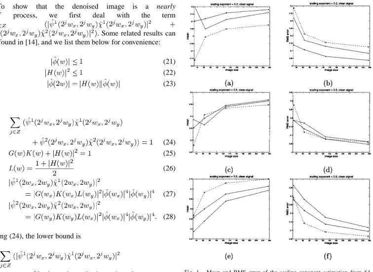
Fig. 1. Mean and RMS error of the scaling exponent estimation from 64 realizations of clean fBm images with various sizes. “*” and “+” indicate the results obtained by using the proposed 2-D estimation method with Haar and Mallat wavelet, respectively. “o” denotes the result obtained by using 1-D WO’s method with Haar wavelet. (a), (b) Estimation of = 0:2. (c), (d) Estimation of = 0:5. (e), (f) Estimation of  = 0:8.

We can see that the summation term is between the upper and lower bounds; therefore, we have recovered a nearly process.

Finally, we make a comparison between our algorithm and the spatial-domain estimation. Wiener filtering is equivalent to the spatial-domain minimum MSE estimation. Due to the non-stationarity of fBm, direct application of Wiener filtering to the noisy fBm is extermely computationally complex in the spatial domain, since it involves the factorization of a correlation matrix that is not Toeplitz. However, our approach is to apply Wiener filter at each scale in the wavelet domain, in which the noisy

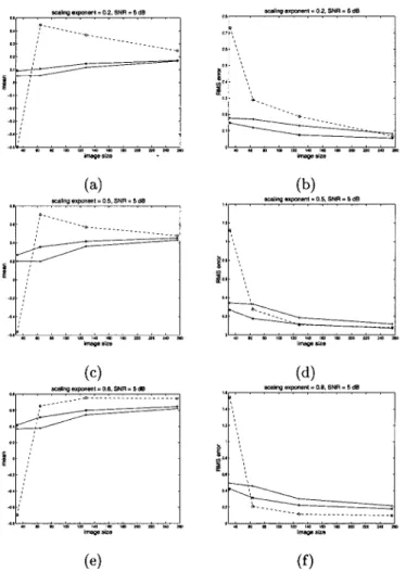
Fig. 2. Mean and RMS error of the scaling exponent estimation from 64 realizations of noisy fBm images with various sizes. Noise was added to image such that SNR= 5 dB. “*” and “+” indicate the results obtained by using the proposed 2-D method with Haar and Mallat wavelet, respectively. “o” denotes the result obtained by using 1-D WO’s method with Haar wavelet. (a), (b) Estimation of = 0:2. (c), (d) Estimation of  = 0:5. (e), (f) Estimation of  = 0:8.

fBm is stationary as proved. Although the cross-scale depeden-cies are ignored in our method, our approach is more computa-tionally efficient.

IV. SIMULATIONRESULTS ANDAPPLICATIONS

In this section, we will first demonstrate the simulation results of our algorithms. Then, the applications on coastline detection and texture segmentation are shown.

A. Simulation Results

For the simulation process, the discrete version of the isotropic 2-D fBm synthesis was given by [11]. The increments of the 2-D fBm are first synthesized by discrete Fourier trans-form, and then the fBm image is added from the incremental values. This method cannot produce 2-D fBm images with exact fBm statistics, but is claimed by the authors to have almost perfect fBm statistics and fast implementation. A constant parameter is set as 0.5 in the synthesis process. 64 fBm realizations of image size 256 256, with each scaling exponent and are generated. Smaller image

Fig. 3. SNR gain from denoising the image with various SNR using Mallat wavelet. (a) Image of size 2562 256. (b) Image of size 128 2 128. “+,” “o,” and “*” indicate the results obtained of fBm with = 0:8; 0:5; and 0:2, respectively.

sizes of 128 128, 64 64, and 32 32 are generated by cutting out the central part of the 256 256 images. Note that the above generated discrete 2-D fBm is the periodic sampling of the continuous fBm, that is,

where is the sampling period. When we take the discrete sampling fBm as the input to the discrete wavelet transform [13], our derivation of (9) based on the continuous wavelet transform would be slightly biased on the fine scales, according to the extension of the results shown in [5]. This bias effect would be reduced in our parameter estimation process by the use of least median of squares method.

In our implementation of wavelet transform, we followed the approach described in [13], [19], where no decimation was ap-plied to the detailed images in both the horizontal and vertical directions. We then estimated the scaling exponent in both

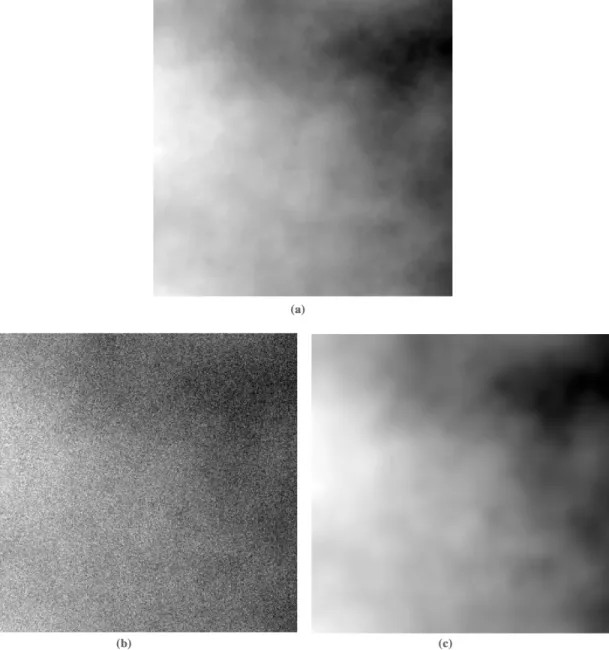
Fig. 4. Image denoising example. (a) 2562 256 fBm image with  = 0:8. (b) Noisy fBm with SNR = 5 dB. (c) Denoised fBm image with SNR gain 21.12 dB.

directions from the detailed images. They were expected to be close in magnitude because we used the isotropic 2-D fBm im-ages, which had the same scaling exponent in all directions sta-tistically. We then took the average of the scaling exponents in these two directions as the scaling exponent of the whole fBm image. In all the experiments, we adopted two wavelets, the Haar wavelet and Mallat wavelet [14], for comparison of filter performance. An image size of was decomposed up to scales. Using the least median of squares method, only the data on half of the scales were selected. , , and were calculated from the data of the selected scales using in-ternal penalty method. As a comparison, we implemented the Wornell and Oppenheim’s 1-D fBm estimation algorithm [21] by using Haar wavelet to estimate the fractal parameters of the 2-D fBm images. For an image, we estimated the fractal parameters of 1-D traces both along the horizontal and ver-tical directions. The total estimated values are then averaged to obtain an estimation of the image.

White noise was added to the fBm images so that the signal-to-noise ratio SNR was 5 dB. The mean and root mean square (RMS) errors of the estimated are plotted in Figs. 1 and 2 as a function of the image size for various values of . From the results of parameter estimation of clean fBm images shown in Fig. 1, we can estimate the scaling exponent precisely for image sizes larger than 128 128. The degree of the RMS error is about 10 . This result is comparable to that of another proposed method [9], in which the same 2-D fBm generation process was used. As reported in [9], the underestimation of with a true value 0.8 was also observed by our experiments. The performance of the Haar wavelet was slightly better than that of the Mallat wavelet because Mallat wavelet has longer support, which introduces unwanted boundary effects in smaller images. In the case of a noisy environment, our method still estimates well for image sizes larger than 128 128. The estimation error is about 10 worse than that in the case of clean image, showing the robustness of our method to added

(a)

(b) (c)

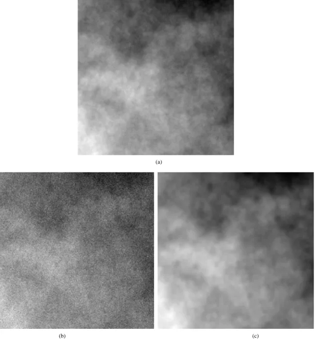
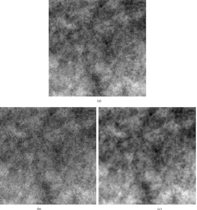
Fig. 5. Image denoising example. (a) 2562 256 fBm image with  = 0:5. (b) Noisy fBm with SNR = 5 dB. (c) Denoised fBm image with SNR gain 13.33 dB.

noise. In all cases, our method always produces estimates of that are distinguishable from each other if their true values are originally different. This is a good property if we do not require precise estimation, but robust estimation that can still distinguish one fBm region from another, for example, in the application of texture image segmentation [22]. The results show that our proposed 2-D estimation method outperforms 1-D estimation method for small images. The computational complexity of 2-D estimation is much less than that of the 1-D estimation, since the 1-D estimation has to be applied to several 1-D traces in the image.

The performance of the image denoising algorithm described in Section III was also evaluated. In order to distinguish the error introduced by parameter estimation and the image denoising al-gorithm, we set a prior the true parameters and in the Wiener filter formula (18) in the experiments. The Wiener filter

was applied to each scale of wavelet transform. Then, the de-noised fBm image was generated by means of wavelet synthesis of the filtered wavelet transform images. Sixty-four realizations of fBm images, with sizes of 256 256 and 128 128, and scaling exponents of 0.8, 0.5, and 0.2, were used. The SNR gain, which is the reconstructed image’s SNR minus the original SNR, was measured by taking the average of 64 SNR gains for each case described above. The Mallat wavelet [14] was used in our experiments. The results are shown in Fig. 3. Images of size 256 256 have about 2 to 3 dB more SNR gains than those of size 128 128 in the case of and . The SNR gain of is higher than that of for about 5 dB, and is higher than for about 5 to 6 dB. The degrading of the denoising effect for small values is due to the smoothing effect of the Wiener filter. The fBm images with lower values represent rougher surfaces [16], and exhibit

sim-(a)

(b) (c)

Fig. 6. Image denoising example. (a) 2562 256 fBm image with  = 0:2. (b) Noisy fBm with SNR = 5 dB. (c) Denoised fBm image with SNR gain 3.48 dB.

ilar behavior with respect to noises. Therefore, the Wiener filter not only smoothes out the added noises, but also smoothes out the original roughness of the fBm images. The low SNR images have better SNR gains after denoising.

For visual evaluation, we present some sample figures of image denoising in Figs. 4–6. The 256 256 fBm images with and , were added with noises such that the noisy fBm had an SNR value of 5 dB. We can see that all denoised results are visually acceptable. In the following, we demonstrate two applications for fbm image parameter estimation and denoising. In both applications, we used the Haar wavelet to process the data.

B. Application 1: Coastline Detection

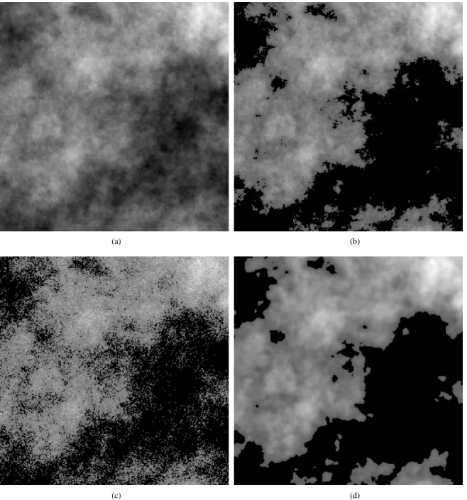
The first application of fBm image denoising is a model of a terrain surface. In order to identify the coastline, we set those

pixel values below a certain threshold to black as if they were below sea level. For example, Fig. 7(a) is an fBm image with , and Fig. 7(b) is the result of coastline detection. If the image is added with white noise, then simple thresh-olding cannot identify the coastline well. This is clearly shown in Fig. 7(c), where 5 dB noise was added to the image shown in Fig. 7(a). One can observe many dotted noises, and that the coastline cannot be identified clearly. In Fig. 7(d), we show the result of coastline detection on the denoised image using our al-gorithm. It is a smoothed version of the original coastline shown in Fig. 7(b), but shows essential topographical features com-paring to Fig. 7(c). For this application, one may simply filter the noisy fBm image with a low-pass filter and threshold the resultant image for the denoised coastline. However, the param-eters of the low-pass filter are usually hard to determine and the resultant smoothed image is not an process. Besides, the

(a) (b)

(c) (d)

Fig. 7. Example of coastline detection. (a) Original 2562 256 fBm image with  = 0:5. (b) Coastline detection of original fBm image. (c) Coastline detection of the noisy fBm with SNR= 5 dB. (d) Coastline detection of the denoised fBm image.

knowledge of the fBm and noise is not used in this approach. Therefore, low-pass filtering is not a suitable solution compared with our denoising approach.

C. Application 2: Texture Segmentation

The estimated fractal parameter can be used as a useful feature for texture segmentation and classification. In this sec-tion, we will demonstrate its application in texture segmenta-tion. Fig. 8(a) shows a 450 380 image of natural scenes, which by human eyes can be classified into three clusters: a sky, a cloud, and a mountain surface. We used a small sliding window of size 32 32 to estimate the scaling exponent , and the center pixel of this window was assigned this estimated value as its local feature. This fractal feature was computed for each pixel,

then this feature image was clustered to obtain the segmented image. A Gaussian filter of variance 6 was used to smooth the resultant feature images. Then, we applied c-mean algorithm to classify each pixel to one cluster, assuming that the number of clusters was given as a priori knowledge. The classified pixels were given gray level N which was equal to their cluster number. This clustered image is shown in Fig. 8(b). Although the cloud can be modeled as an fBm, there are still regions of smooth gray values inside the cloud and these regions are misclassified. The mountain surface and the sky form another areas with different degrees of coarseness. This leads to different fractal parameter

in these areas.

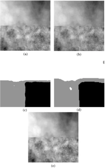
Fig. 9(a) shows a 512 512 texture mosaic created by three fBm images with different scaling exponents : in the upper 256 512 is an fBm image with , in the lower left

(a) (b)

Fig. 8. Segmentation of natural scenes. (a) Original 4502 387 photograph. (b) Texture segmentation result.

Fig. 9. Application of texture segmentation and denoising. (a) Original 5122 512 fBm image mosaic. (b) Noise was added to (a) such that SNR= 10 dB. (c) Texture segmentation result of (a). (d) Texture segmentation result of (b). (e) Denoised image of (b) according to the segmentation result of (d).

corner is a 256 256 fBm image with , and in the lower right corner is a 256 256 fBm image with . One can easily see the texture boundaries. They are not detectable by an edge detection method; too many edge points will be found due to the singular behavior of an fBm. According to our previous experimental result in Fig. 1, in the case of clean fBm param-eter estimation, the degree of the RMS error is below 10 for window size above or equal to 32 32. Therefore, We used sliding window of size 32 32 to estimate the fractal param-eter of the clean fBm mosaic. It had been reported that the fractal feature alone cannot segment texture well [9], especially in the case of noisy environment, in which the parameters cannot be precisely estimated with only local data. So we added the fractal power parameter in (3) as another feature. could be con-verted from in our parameter estimation process, or derived as follows. From the formula of fBm [9]

var

first we compute the - and -directed increments of the fBm

image, that is, and

. Then we calculate the average energy of each of the two increments over a window as the approximation to . These two quantities can be used as local features for the middle pixel in the window. A Gaussian filter of variance 4 was used for smoothing. Then, c-mean algorithm was used to classify the feature images. This clustered image is shown in Fig. 9(c). The major segmentation errors happened in the texture boundaries, in which the parameter estimation is inaccurate.

White noise was added to the fBm mosaic in Fig. 9(a) such that the SNR is 10 dB. This noisy fBm mosaic is shown in Fig. 9(b). From previous experiments in Fig. 2, window size must be greater than 64 64 to achieve better parameter es-timation. We thus chose sliding window of size 64 64. The scaling exponent and the fractal power parameter for each pixel were also estimated. Similar Gaussian smoothing of variance 6

and c-mean clustering method were applied in the noisy fBm mosaic. The clustered result is shown in Fig. 9(d). A more se-vere segmentation error occurs in the texture boundaries. Based on this segmentation result, we will estimate the fBm mosaic. We identified the texture boundaries of the noisy fBm mosaic and partitioned them into three rectangular sub-images. Then, we applied our parameter estimation method to each sub-image for the parameters , , and . We obtained and from the estimated and at each subimage by using (6) and (8), respectively. Finally, the denoised sub-images were obtained by using our proposed Wiener filtering method. The denoised fBm mosaic is shown in Fig. 9(e). The SNR of the denoised fBm mo-saic is about 17.21 dB. Thus, we have about 7 dB gain from the segmentation and denoising process.

V. CONCLUSION

We have showed that the wavelet transform of a 2-D fBm at each scale is WSS. A new fractal estimation method, based on the decay of the variance of the wavelet transform of a noisy fBm image across scales, has been proposed. This new method allows estimation of the fractal parameter on small image blocks, and outperforms many conventional fractal parameter algorithms on small images, where the fractal parameter is obtained by averaging the 1-D results in many directions using 1-D fractal estimation algorithm.

For the estimation of a denoised image, a Wiener filter was applied to the noisy wavelet transform on each scale. Then, a smoothed “denoised” image was obtained after applying the inverse wavelet transform. We have shown that the averaged power spectrum of the estimated image is isotropic and is a

nearly process. Finally, we demonstrated our algorithms on the applications of coastline detection and texture segmenta-tion. Further extension of this work to wider classes of scaling processes is under investigation.

REFERENCES

[1] D. P. Bertsekas, Constrained Optimization and Lagrange Multiplier

Methods. New York: Academic, 1982.

[2] C. Chen, J. S. Deponte, and M. D. Fox, “Fractal feature analysis in med-ical imaging,” IEEE Trans. Med. Imag., vol. MI-8, pp. 133–142, 1989. [3] N. Delprat, B. Escudie, P. Guillemain, R. Kronland-Martinet, P.

Tchamitchian, and B. Torresani, “Asymptotic wavelet and Gabor analysis: Extraction of instantaneous frequencies,” IEEE Trans. Inform.

Theory, vol. 38, Mar. 1992.

[4] P. Flandrin, “On the spectrum of fractional Brownian motions,” IEEE

Trans. Inform. Theory, vol. IT-353, pp. 197–199, Jan. 1989.

[5] P. Flandrin, “Wavelet analysis and synthesis of fractional Brownian mo-tion,” IEEE Trans. Inform. Theory, vol. 38, Mar. 1992.

[6] W. L. Hwang and S. Mallat, “Characterization of self-similar multifrac-tals with wavelet maxima,” Appl. Comput. Harmon. Anal., vol. 1, pp. 316–328, 1994.

[7] W. L. Hwang, “Estimation of fractional Brownian motion embedded in a noisy environment using nonorthogonal wavelets,” IEEE Trans. Signal

Processing, vol. 47, Aug. 1999.

[8] L. Kaplan and C.-C. Kuo, “Fractal estimation from noisy measurements via discrete fractional gaussian noise and the Haar basis,” IEEE Trans.

Signal Processing, vol. 41, Dec. 1993.

[9] , “Texture segmentation via Haar fractal feature estimation,” J. Vis.

Commun. Image Represent., vol. 6, Dec. 1995.

[10] , “Texture roughness analysis and synthesis via extended self-sim-ilar (ESS) model,” IEEE Trans. Image Processing, vol. 4, Nov. 1995. [11] , “An improved method for 2-D self-similar image synthesis,” IEEE

Trans. Image Processing, vol. 5, May 1996.

[12] T. Lundhal, W. J. Ohley, S. M. Kay, and R. Siffert, “Fractional Brownial motion: An ML estimator and its application to image texture,” IEEE

Trans. Med. Imag., vol. MI-5, Sept. 1986.

[13] S. Mallat and W. L. Hwang, “Singularity detection and processing with wavelets,” IEEE Trans. Inform. Theory, vol. 38, Mar. 1992.

[14] S. Mallat and S. Zhong, “Characterization of signals from multi-scale edges,” IEEE Trans. Pattern Anal. Machine Intell., vol. 14, no. 7, 1992. [15] B. Mandelbrot and H. Van Ness, “Fractional Brownian motions,

frac-tional noises and applications,” SIAM Rev., vol. 10, Oct. 1968. [16] A. P. Pentland, “Fractal-based description of natural scenes,” IEEE

Trans. Pattern Anal. Machine Intell., vol. PAMI-6, pp. 661–674, Nov.

1984.

[17] K. Perlin, “Hypertexture,” Comput. Graph., vol. 23, July 1989. [18] P. J. Rousseeuw, “Least median of squares regression,” J. Amer. Statist.

Assoc., vol. 79, Dec. 1984.

[19] Z. Cvetkovic and M. Vetterli, “Discrete-time wavelet extrema represen-tation: Design and consistent reconstruction,” IEEE Trans. Signal

Pro-cessing, vol. 43, Mar. 1995.

[20] G. W. Wornell, “A Karhunen-Loeve-like expansion for 1/f processes via wavelet,” IEEE Trans. Inform. Theory, vol. 36, pp. 859–861, July 1990. [21] G. W. Wornell and A. Oppenheim, “Estimation of fractal signals from noisy measurements using wavelet,” IEEE Trans. Signal Processing, vol. 40, Mar. 1992.

[22] S. Hoefer, F. Heil, M. Pandit, and R. Kumaresan, “Segmentation of tex-tures with different roughness using the model of isotropic two-dimen-sional fractional Brownian motion,” Int. Conf. Acoustics, Speech, Signal

Processing, 1993.

[23] I. S. Reed, P. C. Lee, and T. K. Truong, “Spectral representation of frac-tional Brownian motion in n-dimensions and its properties,” IEEE Trans.

Inform. Theory, vol. 41, p. 1439, Sept. 1995.

[24] B. F. Wu and Y. L. Su, “On stationarizability for nonstationary 2-D random fields using discrete wavelet transforms,” IEEE Trans. Image

Processing, vol. 7, pp. 1359–1366, Sept. 1998.

[25] A. Arneodo, N. Decoster, and S. G. Roux, “Intermittency, log-normal statistics, and multifractal cascade process in high-resolution satellite images of cloud structure,” Phys. Rev. Lett., vol. 83, pp. 1255–1258, Aug. 1999.

Jen-Chang Liu received the B.S. and M.S. degrees in

computer science and information engineering from National Chiao Tung University, Hsinchu, Taiwan, R.O.C., in 1994 and 1996, respectively. He is cur-rently pursuing the Ph.D. degree in electrical engi-neering at National Taiwan University, Taipei.

He is a Research Assistant in the Institute of Information Science, Academia Sinica, Taiwan. His research interests include audio/image compression and wavelet theory.

Wen-Liang Hwang received the B.S. degree in

nu-clear engineering from National Tsing Hua Univer-sity, Taiwan, R.O.C., the M.S. degree in electrical en-gineering from Polytechnic Institute of New York, Brooklyn, and the Ph.D. degree in computer science from New York University in 1993.

He was a Postdoctoral Researcher with the De-partment of Mathematics, University of California, Irvine, and a Scientist with a network management company. He became a Member of the Institute of Information Science, Academia Sinica, Taiwan, in January 1995. His research emphasizes on the applications of wavelet transform in signal and image processing.

Ming-Syan Chen (S’88–M’88–SM’93) received the

B.S. degree in electrical engineering from National Taiwan University (NTU), Taipei, Taiwan, R.O.C., in 1982, and the M.S. and Ph.D. degrees in computer, information, and control engineering from the Uni-versity of Michigan, Ann Arbor, in 1985 and 1988, respectively.

He is currently a Professor with the Electrical En-gineering Department, NTU, Taipei. He was a Re-search Staff Member with IBM T. J. Watson ReRe-search Center, Yorktown Heights, NY, from 1988 to 1996. His research interests include multimedia systems, data mining, and multimedia networking. He has published more than 85 papers. In addition to serving as a program committee member in many conferences, he was program chair/co-chair of VLDB-2002 and the ICS Workshop on Computer Networks, Internet, and Multimedia in 1998 and 2000. He was a keynote speaker on Web data mining at the International Computer Congress in 1999 and a tutorial speaker on parallel databases at DASFAA-1999. He holds, or has applied for, 17 U.S. patents in the areas of interactive video playout, video server design, and con-currency and coherency control protocols.

Dr. Chen is an editor on data mining and parallel database areas for the IEEE TRANSACTIONS ONKNOWLEDGE ANDDATAENGINEERING. He was also a guest co-editor for the IEEE TRANSACTIONS ONKNOWLEDGE ANDDATA ENGINEERING, special issue on data mining, in December 1996. He was a distinguished visitor of IEEE Computer Society for Asia-Pacific in September 1998, program chair for the IEEE ICDCS Workshop on Knowledge Discovery and Data Mining in the World Wide Web in 2000, and a tutorial speaker at the 11th IEEE International Conference on Data Engineering in 1995. He received the Outstanding Innovation Award from IBM Corporate in 1994 for his contribution to parallel transaction design and implementation for a major database product, and numerous awards for his inventions and patent applications. He is a member of ACM.