Chapter 1
Introduction
1.1 Role of Simulation-Based Functional Validation
While silicon capacity continues to increase and the size of devices and the minimal width of lines are decreasing rapidly, Integrated Circuit (IC) designers could integrate many functions, even a whole complex system, into a single chip. A typical single SoC may consist of millions of logic gates, raising the immense potential for design errors and thus significantly complicating the verification task. Verification is now perceived as the major bottleneck in integrated circuit design [1,2].
Formal verification techniques have partially alleviated this problem. These techniques use mathematical or formal techniques to exactly prove or disprove the properties about a hardware design. Equivalence checking [3,4,5] attempts to prove that the two compared designs (the specification and the implementation) are logically equivalent. A popular use of this kind of techniques is to verify that the gate-level netlist, which is often generated by a synthesis tool, correctly implements the original Hardware Description Language (HDL) codes. In this usage case, equivalence checking can be quite useful to ensure the conformance of the synthesis results. Nevertheless, to verify the correctness of the initial register-transfer level (RTL) HDL descriptions requires other approaches.
It often operates directly on Binary Decision Diagrams (BDDs) to formally prove or disprove some properties or assertions of a hardware design. Due to the rapid progress of SATisfiability solver (SAT solver), recently researches of model checking [9,10] tend to exploit SAT solvers instead of BDDs. These model checkers may be so powerful that they can determine whether some deadlock conditions may occur or they can formally verify relates to interfaces. Although the formal techniques for language containment, model checking, property checking, and assertion-based verification [11] are making progress on the problem of verifying the correctness of the initial HDL codes, there is no indication that these techniques will be able to offer comprehensive verification across a wide variety of designs. For this reason, and perhaps because of the intuitive appeal of simulation, it appears that simulation-based functional validation is still one of the popular means for design verification for some time to come.
Nevertheless, functional validation based on simulation can be only partially completed. To address this incompleteness, coverage-driven semiformal methods have been developed. These methods exert better control over simulation by using various schemes to generate input stimuli and assess the extent of verification completeness. The goal is to achieve comprehensive validation without wasted efforts. Coverage metrics drive simulation resources to right direction and help approximate the goal.
1.2 Classification of Coverage Metrics for Validation on
HDL Descriptions
1.2.1 Code Coverage Metrics
The problem of verifying the correctness of Design Under Validation (DUV) described in a HDL using simulation is similar to the software testing problem because a HDL description is quite similar to a program written in a high-level programming language like C. As a result, code coverage metrics for HDL codes are largely derived from metrics used in software testing. They are mainly used to identify which code structure classes in the HDL code are exercised during simulation.
These code structures are defined on a Control Flow Graph (CFG), which is a graphical representation of a program’s control structure [12, Ch. 3]. Given a set of program stimuli, one can determine the code structures of the HDL code activated by the stimuli. The simplest one should be line or statement coverage metric. The line coverage metric measures the number of times every statement is exercised by the program stimuli. More sophisticated code-based coverage metrics are branches,
expression, and path coverage. These code coverage metrics involve the CFG
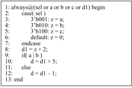
corresponding to the HDL code. Control statements constitute the branching point in the CFG. We use the following Verilog code fragment shown in Figure 1-1 to illustrate each aforementioned code coverage metrics.
Figure 1-1: A HDL code example
The if statement on line 9 has (a | b) as the control expression. Branch coverage metric requires exercising each possible direction from a control statement. For the if statement, lines 10 and 12 must both be executed during a simulation run. Similarly, for the case statement on line 2, lines 3, 4, and 5 must be executed.
A more sophisticated metric, expression coverage metric, requires exercising all the possible ways that an expression can yield each value. For instance, for the control expression (a | b), in addition to the case where a = 0 and b = 0, we must exercise the two separate cases where the expression gives 1. The first case is a = 1 and b = 0 and the other is a = 0 and b = 1.
Path coverage metric refers to paths in the CFG. For instance, in the Verilog
example, the branch of the case statement on line 4 followed by the else branch of the if statement defines one path through the CFG. The branch of the case statement on
line 5 followed by the true branch of the if statement is another path through the CFG.
1: always@(sel or a or b or c or d1) begin
2: case( sel )
3: 3’b001: z = a;
4: 3’b010: z = b;
5: 3’b100: z = c;
6: default: z = 0;
7: endcase
8: d1 = z + 2;
9: if( a | b )
10: d = d1 + 5;
11: else
12: d = d1 – 1;
13: end
A potential goal of software testing is to have 100% path coverage, which implies 100% branch and line coverage. However, 100% path coverage is a very stringent requirement and the number of paths in a program may be exponentially related to program size. For this reason, exercising all paths may be impossible. Representative subsets are usually chosen by verification engineers or circuit designers with some heuristics.
Measuring the aforementioned code coverage metrics requires little overhead, and because of the ease of interpreting coverage results, these metrics are popularly used nowadays. Almost all design groups use some form of code coverage, and many commercial tools are available to measure them. Nevertheless, unlike the case with software, achieving certain extent of code coverage for hardware is a minimum requirement because that hardware designs are highly concurrent. More than one code fragment is active at a time, thus fundamentally distinguishing HDL code from sequential software. The aforementioned code coverage metrics do not address this essential hardware characteristic. Consequently, requiring complete code coverage for hardware, although necessary, is not enough.
1.2.2 Coverage Metrics Based on Circuit Structure
Toggle coverage should be the simplest metric that is based on circuit structure. The metric requires that each wire in the circuit switches from 0 to 1 or 1 to 0 at some time instances during simulation. This metric can identify physical portions of the DUV that are not properly exercised. Many other sophisticated metrics in this class
are developed based upon toggle coverage.
Separating circuits into data path and control logics is reasonable for defining more useful circuit-structure based metrics. In the data path portion, registers deserve special attention during validation. Each register must be initialized, loaded, and read from, and each feasible register-to-register path must be exercised.
Coverage metrics of this class are defined on exercising the concerned circuit structures. Like code coverage metrics, they are easy to measure and intuitive to interpret and thus are popular. However, circuit-structure coverage metrics are defined on static, structural representations; hence their ability to quantify and pose requirements on sequential behavior is limited. As a result, similar to code coverage metrics, circuit-structure based metrics only provide a lower bound validation requirement as well.
1.2.3 Coverage Metrics Defined on Finite State Machine
In order to quantify and pose requirements on sequential behavior of the DUV, metrics defined on state transition graphs are developed and they are truly more powerful in this regard. These metrics require state, transition, or limited path coverage on a finite state machine (FSM) system representation;
Because FSM descriptions for complete systems are prohibitively large, these metrics must be defined on smaller, more abstract FSMs. We classify FSMs into two broad categories:
2. FSMs automatically extracted from the design description. Typically, after a set of state variables is selected, the design is projected onto this set to obtain an abstract FSM.
Metrics in the first category are less dependent on implementation details and encapsulate the design intent more succinctly. However, constructing the abstract FSM and maintaining it as the design evolves takes considerable effort. Moreover, there is no guarantee that the implementation will conform to the high-level model. Despite these drawbacks, specifying the system from an alternative viewpoint is an effective method for exposing design errors. Experience shows that using test scenarios targeted at increasing this kind of coverage has detected many difficult-to-find bugs [14].
In the second category, the state variables of the abstract FSMs for metrics can be selected manually or with heuristics. Shen and Abraham present a heuristic technique for extracting the control state variable that changes most frequently, called the primary control state [15]. They compute an FSM reflecting the transitions of the primary control state variable and require coverage of all paths of a certain length in this FSM. Even small processors have a large number of such paths, but because each simulation run is short, the cost is tolerable. Kantrowitz and Noack use transition coverage on a hand-constructed abstract model of the system, as well as cache interface logic. Others select important, closely coupled control state variables based on the design’s architecture [14,16].
Selecting abstract FSMs requires compromising between the amount of information that goes into the FSMs and the ease of using the coverage information.
The relative benefits of the choice of FSMs and the metrics defined on them are design dependent. Increasing the amount of detail in the FSMs increases the coverage metric’s accuracy but makes interpreting the coverage data more difficult. If the abstract FSM is large, attaining high coverage with respect to the more sophisticated metrics is difficult.
The biggest challenge with state-space-based metrics is writing coverage-directed tests. Determining whether certain states, transitions, or paths can be covered may be difficult. The FSMs’ state variables may be deep in the design, and achieving coverage may require satisfying several sequential constraints. Moreover, inspecting and evaluating the coverage data may be difficult, especially if the FSMs are automatically extracted. Some automated approaches involve sequential testing techniques [17]. Others establish a correspondence between coverage data and input stimuli using pattern matching on previous simulation runs. The capacity of automated methods is often insufficient for handling coverage-directed pattern generation on practical designs, whereas the user may need to understand the entire design to generate the necessary inputs. Nevertheless, state-space-based metrics are invaluable for identifying rare, error-prone execution fragments and FSM interactions that may be overlooked during simulation, thus justifying the high cost of test generation. Ultimately, carefully choosing abstract FSMs can alleviate many of the problems mentioned.
Coverage metrics of this class consider about exercising states, state transitions, and a particular sequence of transitions of the targeted FSM. As with code coverage, circuit-structure based ones, metrics of this class do not explicitly consider whether
erroneous effects caused by exercising some internal error portions of the DUV can be revealed during simulation.
1.3 Observability Issue in Simulation-Based Functional
Validation
In a simulation-based validation framework, the simulation results or values should be compared against the correct values on some signals of interest to check the correctness of circuit behaviors. The correct values of these signals of interest may come from a reference model described at a different abstraction level or monitors and assertions. These signals of interest are called Observation Points (OPs) because they act like observation windows to uncover bugs in the DUV. During simulation, a discrepancy from the desired behavior is detected only if an OP takes on a simulation value that conflicts the correct value specified by the reference model.
Typically, OPs are Primary Outputs (POs) of the DUV and/or some other internal wires or register outputs that are selected by circuit designers. Designers usually follow their understanding to the specification and the behavior of the circuit to select these OPs, without explicit consideration of error propagation, i.e. whether erroneous effects of some internal signals caused by design errors are propagated to OPs. As a result, during simulation process, even if some erroneous values were generated by some activated internal bugs, the erroneous values may be masked during their propagation to Ops, causing that these erroneous values as well as the internal bugs remain undetected.
Traditional code coverage metrics from software testing, such as statement
coverage, branch coverage, and path coverage metrics, only consider whether their
concerned code structures are exercised. Circuit-based coverage metrics or FSM coverage metrics also do not explicitly check whether erroneous effects can be propagated to OPs for bug detection during simulation. They all do not explicitly consider whether erroneous effects caused by internal bugs are propagated to OPs. Design errors may be masked and still remain undetected even if they were said “covered” under these coverage metrics. The result is that verification completeness is overestimated by these coverage metrics.
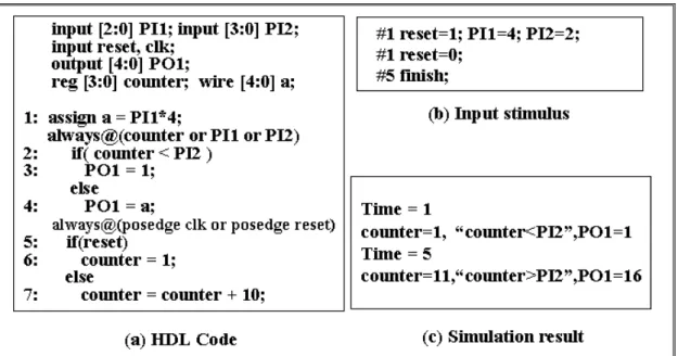
We use the following example to explain the error masking situation. If we simulate the HDL code fragment shown in Figure 1-2(a) with the input stimulus given in Figure 1-2(b), the simulation result is as shown in Figure 1-2(c). As far as code coverage metrics are concerned, we will find that with respect to statement, branch, and path coverage metrics, 100% coverage is achieved. If the three coverage metrics are used to evaluate the extent of the simulation, the input stimulus in Figure 1-2(b) should be regard as a good test vector set for the design in Figure 1-2(a) since the test vector set exercises every target code structures during simulation.
Figure 1-2: An example of functional validation on a HDL code fragment
However, assumed that statement 7 is carelessly written into “counter=counter+2”, we surprisingly find that this careless design error can not be detected by this input stimulus of quality. Although the design error “counter=counter+2” changes the value of counter into 3 at Time = 5, different from the expected value 11, value 3 and value 11 cause the same evaluation result in the operation “counter<PI2”. The erroneous value 3 is masked. The design error in statement 7 hides from being detected. In this case, the completeness of simulation is misjudged by the three coverage metrics. Therefore, observability consideration is important to suitably assess the comprehensiveness of validation.
The Observability-based Code COverage Metric (OCCOM) is the pioneer that addresses the essential observability issue [18]. Dump-file based OCCOM computation facilitates integration with commercial simulators and thus accelerates the analysis process [19]. Tag-based observability measures are extended to assess the
extent of validation for C programs in recent works [20]. Test pattern generation approaches for OCCOM make the entire work more practical [21].
In the above OCCOM approaches, two special tags, Δ and - Δ, are injected on each signal to simulate potential increasing and decreasing value changes caused by some bugs. These tags on variables are not tied to particular design errors. The propagation of tags is used to simulate the propagation of potential erroneous effects. The percentage of tags that can be propagated to OPs is the coverage of OCCOM. However, tags can only be observed or unobserved, providing only two levels of measurement; 1 and 0. Erroneous effects that have lower observation opportunities may still be judged as observable. Thus, verification completeness may still be overestimated by OCCOM. If a new observability measure for HDL descriptions could provide intermediate values between 1 (observed) and 0 (unobserved), the likelihood of misestimating observability should be reduced.
1.4 Other Observability-Related Researches
1.4.1 Testability Analysis in Manufacturing Test
Manufacturing test is a process of checking that integrated circuits are manufactured correctly. The basic premise is the modeling of manufacturing defects as logical faults. Since manufacturing is a physical process that can be analyzed, credible fault models can be derived. For example, defects are known to cause breaks and shorts in metal wires. These breaks or shorts can be modeled as logical faults
since there is a direct correspondence between wires in silicon and connections in the logic circuit.
One of the most popular fault models in manufacturing test is the stuck-at fault model [22]. The stuck-at fault model is a logical fault model where any wire in the logic circuit can be stuck-at-1 or stuck-at-0. A test vector that produces the opposite value (zero for a stuck-at-1, and one for a stuck-at-0) will excite the fault. The effect of the fault has to be propagated to an observable circuit output in order for the fault to be detected by the vector.
The direct correspondence between a metal wire in the silicon integrated circuit and a connection in the logic circuit motivates logical fault models. No such correspondence may exist for a behavioral description in an HDL or structural RTL description. Statements in the HDL description may correspond to hundreds of gates and wires in the final design.
Based on the fault models, test vectors are generated and applied to test manufactured integrated circuits. Fault coverage analysis is then conducted to judge whether the integrated circuits are well tested or not. Testability here is used to guide test pattern generation or as a direct substitution of a fault coverage report. Observability is often defined as the difficulty of observing erroneous effects caused by some bit-level stuck-at-faults [23]. Recent researches abstracted defects as higher-level logical fault models [24,25,26].
However, the correspondence between logical fault models and HDL design errors is still weak in two aspects. First, an erroneous statement may be synthesized into hundreds of erroneous gates and erroneous wires. Second, there are almost no
credible design error models for HDL descriptions. Thus, logical fault models hardly link to HDL design errors. Testability for these logical fault models consequently differs from the observability for HDL descriptions.
Some RTL testability analysis research exploits the idea of hierarchical testing with a pre-computed test vector set [27,28]. These studies define testability as the difficulty of generating input patterns for RTL circuits or instructions for processors to test internal RTL modules. They are different from the observability measures used to measure the likelihood of error propagation.
1.4.2. Sensitivity Analysis in Software Testing
In software testing arena, a sensitivity analysis, also called PIE analysis, for software programs to locate hard-to-detect bugs in a software program was proposed by J. Voas [29]. PIE analysis uses program instrumentation, syntax mutation, and changed values injected into data states to predict a location’s ability to cause program failure if the location were to contain a fault. The program inputs are selected at random consistent with an assumed input distribution. This analysis does not require a testing oracle because PIE analysis uses the program itself as an oracle for examining the output of altered versions of the program.
The PIE analysis estimates the below three probabilities to predict a software program’s dynamic computational behavior as well as where hard-to-detect bugs may hide. The three probabilities are 1) Execution probability - the probability that a location is executed, 2) Infection probability - the probability that a change to the
source program causes a change in the resulting internal computational state, and 3)
Propagation Probability - the probability that a forced change in an internal
computational state propagates and causes a change in the program’s output.
Among the three probabilities, the propagation probability (PP) of a variable is the estimated probability that a variable’s erroneous values caused by some bugs are observed in the program outputs. Propagation Probability is a good observability measure for software programs, even for HDL programs. The PP of a variable v in the program is estimated by a statistics-based approach, repeatedly infecting the data state of v (injecting erroneous values on variables in memory) and simulating the program. The ratio of the number of program failures to total number of experiments is the PP of v. This PP measures are quite accurate estimations for the likelihood of error propagation (observability for erroneous effects). However, the proposed statistical computation approach requires too much time and thus may be unsuitable for HDLs of commercial products because time to market is always important for commercial products.
1.5 Design Error Diagnosis on Faulty HDL Descriptions
1.5.1 Traditional Design Error Diagnosis Works
Due to the high complexity of modern Very Large Scaled Integrated (VLSI) circuit designs, verification process may often find that a design in the current stage (implementation) is not consistent with that in the previous stage (specification). Once
a functional mismatch is found, design error diagnosis is needed.
Most of the previous studies on this topic target the diagnosis of gate-level or lower-level implementations. These methods can be roughly divided into two categories: simulation-based approaches and symbolic approaches. Simulation-based approaches [30,31] first derive a set of input vectors that can differentiate the implementation and the specification. These binary or three-valued input vectors are called erroneous vectors. By simulating each erroneous vector, the possible error candidates can be trimmed down gradually. The heuristics to filter out impossible error candidates vary from one to another. Some of them rely on error models such as gate errors (missing gate, extra gate, wrong logical connective,…) and line errors (missing line, extra line,…) while other approaches are structure-based methods and require no error models.
On the other hand, symbolic approaches [32,33] do not enumerate erroneous vectors. They represent symbolic functional manipulation with Ordered Binary Decision Diagram (OBDD) to formulate the necessary and sufficient condition of fixing a single error. Based on these formulations, every potential error source can be precisely identified. An approach to combine the both symbolic and simulation-based techniques has also been proposed to reduce the run time of design error diagnosis. In comparison, the symbolic approaches are accurate and extendible to multiple design errors. However, constructing the required BDD representations may cause memory explosion when applied to large circuits. On the other hand, simulation-based approaches, although scale well with the size of circuits, are often not accurate enough. In order to avoid potential memory explosion of BDD-based symbolic
approaches, some recent symbolic works exploit the progress of Boolean satisfiability (SAT) solver and develops SAT-based approaches [34].
1.5.2 Software Debugging Techniques
In addition to gate-level or other lower-level implementations, design errors can also occur at the very first design stage – modeling the circuit behavior using HDLs. Traditionally, debugging a faulty HDL design relies on manually tracing the faulty HDL code. However, a simple HDL design today can have probably thousands of code lines and even more. Manually tracing the faulty HDL code to debug is not an effective debugging method. Approaches to assist HDL debugging are urgent.
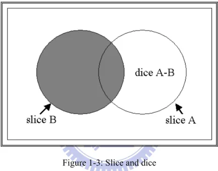
For a Register-Transfer Level (RTL) HDL code, the distance between the HDL code and a software program is small: diagnosis may be seen as a software problem as well as a hardware one. In the software diagnosis domain, most of the methods are based on the slicing technique [35,36]. Program slicing, introduced by Weiser [36] is a technique for restricting the behavior of a program to some specified subsets of interest. The main idea behind this technique is to decompose the considered program into independent parts, called slices. Each slice contains all the statements that could have influenced the value of a variable at a given program point. It can be executed separately from the rest of the program. The difference between two slices is called a dice and is the basis of the fault location process.
Assume that one of them (B) gives a correct result; whereas the other (A) gives a faulty one. It is obvious that the faulty area will be in the dice A minus B, which is smaller than the area of the faulty slice A. Consequently, the effort of searching in the whole slice A is saved and the diagnosis duration time is reduced.
Figure 1-3: Slice and dice
The process of fault location implies to execute each slice and the correctness of each slice execution has to be determined: a human intervention is generally needed for establishing the oracle (the algorithmic debugger interacts with the user through queries about the intended program behavior). Moreover, in this manner, multiple times of simulation are required before real diagnosis can go on. This is too time-consuming.
1.5.3 Techniques for Debugging HDL Descriptions
In the literature, some researches have targeted on techniques that assist HDL design debugging. Peischl et al [37] focus on Model-Based Diagnosis (MBD) paradigm. They employ structure and behavior with respect to their error models for software debugging. Besides, error-model based approaches, there are also error-model free methods that should have better applicability to various kinds of design errors.
Maisaa Khalil et al [38] proposed an automatic diagnosis approach based on the cross check on the result of each test case. By using four strategies based on different four hypotheses, four error candidate sets are sequentially obtained, from the smallest one to the biggest one. It is expected that tool users or debugging engineers can locate design errors in the first few error candidate sets, whose size are relatively smaller, to save the debugging efforts. However, the first three hypotheses are not always satisfied since design errors in a fault HDL description can be multiple and the oracle can be unsure. True design errors may be absent in the first three error candidate sets, resulting in that the efforts of searching design errors in these sets are wasted. Even worse, we still have to search design errors in the fourth set of error candidates, the largest one.
Shi et al [39] applied data dependency analysis, execution statistics, and the characteristics of HDL operations to filter out impossible error candidates. In this method, only one reduced set of error candidates is derived for examination with a single time of simulation. And, the size of error candidate set (error space) is acceptable in size. Huang et al [40] further exploited the extra observability of
assertions in an attempt to derive smaller error space.
Instead automatic methods to derive error candidates, Y.C. Hsu et al have developed two useful utilities to help designers reason the locality of bugs with manual interventions [41]. However, the number of derived error candidates can still be plenty. Searching design errors among these candidates by examining them one by one blindly may still takes much valuable time.
1.6. Organization
This thesis is organized into five chapters. Chapter 1 gives the introduction to the thesis. Chapter 2 introduces some related works and gives preliminaries. In Chapter 3, we introduce our proposed probabilistic observability measures on HDL designs for efficient functional validation. Besides being used for efficient functional validation, Chapter 4 introduces another application of the probabilistic observability measures on HDL designs - design error diagnosis on faulty HDL descriptions. Finally, we conclude the thesis in Chapter 5 and discuss some future research directions.
Chapter 2
Preliminaries
2.1 Observability-Based Code Coverage Metrics
During simulation-based functional validation, simulation values of Observation Points (OPs) should be compared against the expected values to check the correctness of certain circuit behavior. A discrepancy from the desired behavior can be detected only if some of OPs have simulation values that are different from the expected values. Coverage metrics should explicitly consider the observability requirement (requirement of error propagation) to detect internal design errors such that comprehensiveness of validation can be suitably gauged.
Observability-based Code COverage Metric (OCCOM) is the pioneer that addresses the essential observability issue [18]. A dump-file based OCCOM computation approach is later proposed to facilitate the integration with commercial simulators and thus accelerate the analysis process [19]. In these OCCOM works, two special tags Δ and -Δare injected on each signal to simulate potential increasing and decreasing value changes caused by activated errors. Tag propagation rules are defined for using tag propagation to predict the potential propagation behaviors of these erroneous value changes. The percentage of the tags observed at the OPs is the coverage with respect to OCCOM
approach. The two phases are abstracted as below. We will introduce the two phases individually in detail later in this section.
1) Conditional Statement Transformation: The transformation involves moving some statements and creating new variables to contain extra information during simulation for the next phase calculation. After the transformation, the modified HDL model is then simulated using a standard HDL simulator to obtain a dump-file for the later tag simulation calculus.
2) Tag Simulation Calculus: In this phase of computation, tags are first injected and then the propagation of the injected tags is computed based on the tag simulation calculus developed by the authors [19]. The tag simulation calculus is composed of tag propagation rules for various HDL operations, in which the propagation through the HDL operations is based on likelihoods. For one injected tag, the tag propagation result can be that it is observed at some OPs or it is not observed at any OPs. The third possible result is the presence of special unknown tags ? when the tag propagation is not so sure in the computation.
The conditional statement modifications on the HDL code proposed in [19] are for obtaining sufficient information during HDL simulation for the later tag simulation calculus. Consider a HDL code fragment with a simple conditional statement “if… else …” shown in Figure2-1. The original code fragment is shown on left-hand side and the transformed code is shown to the right in Figure 2-1. Consider the case of a tag on cexp. During the simulation of the modified code, the values of both expr1 and expr2 are computed and stored in the new variables y1 and y2. The new values of y corresponding to the execution of both the then and else clauses are
known, regardless of the value of cexp during simulation. This will help to correctly propagate positive or negative tags on cexp in their tag simulation calculus.
Figure 2-1: A simple conditional statement modification
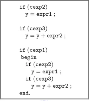
The case of nested conditionals is more complicated. Further, the situation where variables such as y are assigned values that depend on the old values (e.g., increment operation) have to be considered. As an example, consider the Verilog statements shown in Figure 2-2.
Figure 2-2: A nested conditional statement example
Transformation starts with transforming the statement “if(cexp1)”. The result after the transformation on “if(cexp1)” is shown in Figure 2-3. In the next step, the “if(cexp2)” and “if(cexp3)” the statements are transformed. y is the only variable in the original Verilog code whose value is changed inside the if statement and, as a
result, in order to transform the code, a new variable y3 is introduced.
Figure 2-3: Code after first phase of conditional statement transformation
Note that if the value of cexp2 is false, variable y3 is read before assigning any value to it. As a result, it is necessary to initialize its value to the value of y. The transformed code after the entire conditional statement modification is shown in Figure2-4. The transformed code will compute the necessary information to perform propagation of tags on cexp1, cexp2, or cexp3. It can easily be verified that the two pieces of code result in the same values for variable y.
The second phase of OCCOM computation is tag simulation calculus, which is used to predict error propagation and is similar to the D calculus [42]. A tag is represented by the symbol Δ, which signifies a possible change in the value of the variable due to an error. Both positive and negative tags are considered, +Δ written simply as Δ, and -Δ. Both tags are injected onto each internal signal of the DUV first. If the presence or sign of the tag is not known, an unknown tag “?” is used. Note that ? = -? and also 0+? = 1+?.
Tag simulation calculus in [18.19] is based on the likelihood of the propagation of the tag. It is assumed that the tag is propagated or blocked depending on which case is more likely. For example, in the Verilog statement c= (a!=b) with a=2 and b=5, if there is a positive tag on variable a, it is assumed that the tag is not propagated to the variable c [19]. The reason is that the value of the variable c in the presence of the tag is TRUE unless the magnitude of the tag on a is exactly three. As a result, the authors think that it is unlikely to have a tag on variable c. The tag propagation rule for “!=” created in [19] will block the tag from being propagated through this operation.
proposed in [18,19] is briefly introduced in the sequel. For each operator op, after the simulator computes v(f)=v(a)(op)v(b), v(f) might be tagged with a positive Δ or negative -Δ or ? and it is written as v(f)+ Δ, v(f)- Δ, v(f)+?.
1) The calculus for an INVERTER, a two-input AND gate, and a two-input OR gate are shown in Table 2-1, Table 2-2, and Table 2-3, repectively. The five possible values at each input are {0, 1, 0+Δ, 1-Δ, 0+?}. (Note that 0-Δ= 0 and 1+Δ=1.) As an example, if the input of an inverter gate is zero and it has positive tag on it, the value of the output of the inverter will be one and it will have a negative tag on it. The case that the input of the inverter is one and the input has a negative tag is similar. As another example, if one of the inputs of an AND gate is zero and the input has a positive tag and the value of the other input is one and it has a negative tag on it, the value of the output of the AND gate will be zero because the erroneous value of one of the inputs is zero. Using the above calculus, any collection of Boolean gates comprising a combinational logic module can be tag simulated.
Table 2-1: Tag calculus for INVERTER gate in [18,19] INVERTER 0 1 1 0 0 +Δ 1- Δ 1-Δ 0+ Δ 0 + ? 0 + ?
Table 2-2: Tag calculus for AND gate in [18,19] AND 0 1 0+Δ 1- Δ 0+? 0 0 0 0 0 0 1 0 1 0+Δ 1- Δ 0+? 0+Δ 0 0+ Δ 0+ Δ 0 0+? 1-Δ 0 1- Δ 0 1- Δ 0 0+? 0 0+? 0+? 0 0+?
Table 2-3: Tag calculus for OR gate in [18,19]
OR 0 1 0+Δ 1- Δ 0+? 0 0 1 0+Δ 1- Δ 0+? 1 1 1 1 1 1 0+Δ 0+ Δ 1 0+ Δ 1 0+ Δ 1-Δ 1- Δ 1 1 1- Δ 0+? 0+? 0+? 1 0+Δ 0+? 0+?
2) Adder: If all tags on the adder inputs are positive and if the value v(f) < MAXINT, the adder output is assigned to v(f) + Δ. MAXINT is the maximum value possible for f. This is similar if all tags are negative. If both positive and negative tags exist at adder inputs, the output is assumed to be unknown tag. Table 2-4 shows calculus for tag propagation through an adder.
Table 2-4: Tag calculus for ADD (+) Operation in [18,19]
ADDER b b -Δ b +Δ b + ?
a a + b a + b -Δ a + b +Δ a + b +? a -Δ a + b -Δ a + b -Δ a + b +? a + b +? a +Δ a + b +Δ a + b +? a + b +Δ a + b +? a + ? a + b +? a + b +? a + b +? a + b +?
3) Multiplier: All tags have to be of the same sign for propagation. A positive Δ on input a is propagated to the output f provided v(b)!=0 or if b has a positive Δ. The output of multiplier is assigned to v(f) + Δ. This is similar for negative -Δ.
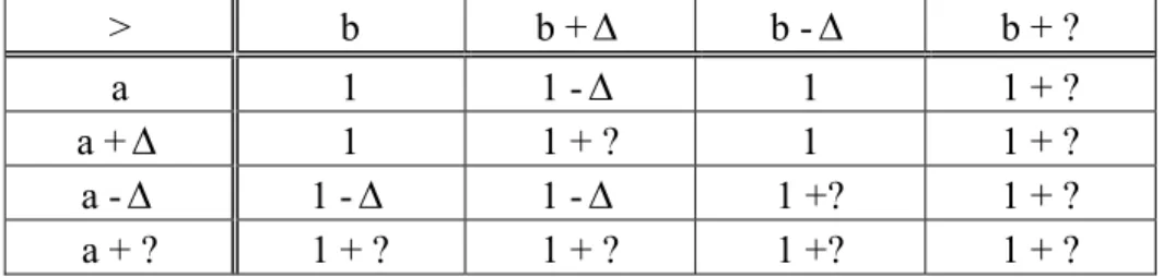
4) Comparators: If tags exist on inputs a and b, they have to be of opposite sign, else the output will have an unknown tag. Assume a positive tag on
a alone or a positive tag on a and a negative tag on b. If v(a) is smaller
than or equal to v(b), then the tag(s) is (are) propagated to the output, else the tag(s) is (are) not. The output of comparator is assigned to 0+Δ. This is similar for other tags and other kinds of comparators. Table 2-5 and Figure 2-6 show the calculus for tag propagation through operator “>” when the result of operation is TRUE and FALSE, respectively. Other tag propagation rules can be found in [18,19,43].
Table 2-5: Tag calculus for “>” when result of a > b is true
> b b +Δ b -Δ b + ?
a 1 1 -Δ 1 1 + ?
a +Δ 1 1 + ? 1 1 + ?
a -Δ 1 -Δ 1 -Δ 1 +? 1 + ?
a + ? 1 + ? 1 + ? 1 +? 1 + ?
Table 2-6: Tag calculus for “>” when result of a > b is false
> b b +Δ b -Δ b + ?
a 0 0 0 +Δ 0 + ?
a +Δ 0 +Δ 0 + ? 0 +Δ 0 + ?
a -Δ 0 0 0 +? 0 + ?
In summary, OCCOM is indeed more stringent than statement coverage metric because it considers only the execution requirement but also the observability requirement to detect internal design errors. The proposed dump-file based OCCOM computation is also an effective approach to derive the OCCOM coverage. In the works, experimental data are also available to demonstrate that the conditional statement modification conducted in the first phase of OCCOM computation introduce very little overhead to HDL simulation. The OCCOM works based on tags indeed provide observability information for effectively and suitably assess the extent of validation. However, tags can only provide two levels of measurement 1 (observed) or 0 (unobserved). A more accurate observability measure is always desirable for the observability issue in simulation-based validation. As the future works in [19] had discussed, the possible future direction they proposed for accuracy improvement of tags are 1) relative magnitude of tag or 2) absolute magnitude of tag.
2.2 PIE Analysis in Software Testing
J.Voas et al [29,44,45] present a dynamic technique to statistically estimate three software program characteristics that affect a software program’s computational behavior: 1) Execution Probability (EP) - the probability that a particular section of a program is executed, 2) Infection Probability (IP) - the probability that the particular section affects the data state, and 3) Propagation Probability (PP) - the probability that a data state produced by that section has an effect on program output. These three characteristics can be used to predict whether faults are likely to be uncovered by software testing.
Among the three probabilities, the third probability PP can be regard as an observability measure for software programs and probably for HDL models as well. PP of a variable a (denoted as PP(a)) is the probability that variable a’s erroneous values caused by some bugs are observed in the program’s outputs and cause program failures. The algorithm to obtain estimated values of PP(a) proposed by J. Voas is abstracted as bellows.
Step1. Set variable count to 0.
Step2. Randomly select an input x according to the input distribution.
Step3. Alter the sampled value of variable a to create a mutant of this program.
Step4. For each different output result in program output after a is changed, increment
count. If a time limit for termination related to the altered state has been exceeded,
increment count. This precaution is necessary because of the effects that altered variables can cause to Boolean conditions that terminate indefinite loops.
Step5. Repeat steps 2-4 n times.
Step6. Divide count by n to derive PP of variable a.
This calculation algorithm to obtain PP(a) is a statistics-based estimation approach. The accuracy of estimated result highly depends on the iteration numbers, n. If n is big enough, the result of this algorithm can be a quite accurate estimation for PP(a). However, it is obvious that to obtain accurate estimations for PP(a) with a big
n requires lots of iteration of simulation as well as computation time. If we intend to
analyze observability of each point in a HDL model using this statistics-based approach, the entire procedure may take too much time. Other approaches or other observability measures are required for the observability analysis for HDL models.
2.3 Error Space Identification Approaches for HDL
Debugging
When verification finds some discrepancy between the specification and the implementation written in a HDL, the debugging process traditionally relies on designers’ manually tracing HDL codes. However, this manual debugging scheme could be tough and time-consuming because a relatively simple HDL design today can have more than thousands code lines. If a reduced set of error candidates can be obtained automatically by some approaches, these approaches should be helpful to this HDL debugging problem.
Maisaa Khalil et al [38] proposed an automatic diagnosis algorithm that contains four hypotheses to diagnose design errors using the HDL information. For systematic analysis, the algorithm classified all possible situations into four hypotheses that are defined from looseness to strictness. The first two hypotheses assume that there is only one erroneous statement in the HDL design. The first ant the third hypotheses assume that the executed statements of correct test cases are impossible to be the error sources. By using four strategies based on different four hypotheses, four error candidate sets are sequentially obtained, from the smallest one to the biggest one. It is expected that tool users or debugging engineers can locate design errors in the first few error candidate sets, whose size are relatively smaller, meaning that searching design errors in the three sets requires less efforts. However, the first three hypotheses do not always stand since design errors in a faulty HDL description can be multiple and the oracle can be unsure. As a result, true design errors may be absent in the first three error candidate sets, resulting in that the efforts of searching design errors in
these sets are wasted. Even worse, it is still required to search design errors in the fourth and the largest set of error candidates. It is also assumed that many test cases can trigger design errors. However, in practice, it is not easy to generate lots of test cases that can trigger the same design errors, especially when designers do not actually know where the design errors are and what they are.
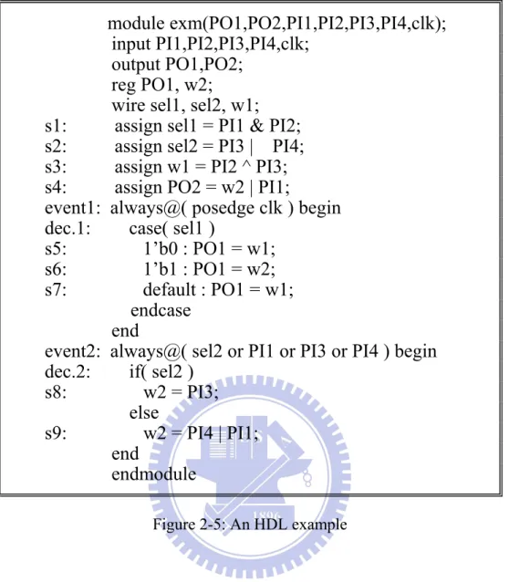
Jiang and et al [46] proposed another error-model free automatic error space identification approach that exploits both data dependency analysis and execution trace to obtain an error space (a reduced error candidate set). The error space is the intersection of the execution trace of EOC (the clock cycle, in which discrepancy between the simulation values of all the primary outputs and the associated expected values is detected) and the result of data dependency analysis on Erroneous Primary Outputs (primary outputs that have simulation values are not consistent with the expected values in EOC). The size of the obtained error space in this approach should be relatively smaller than the one derived by the approach in [38] because additional data-dependency analysis is used to trim down the size. Take the HDL code shown in Figure2-5 as an example to demonstrate the error space identification in [46].
Figure 2-5: An HDL example
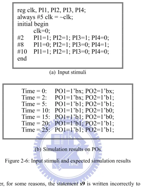
Assume that the code in Figure 2-5 is the correct design that designers expect. The applied input vectors for each time instance and the corresponding values of POs are shown in Figure 2-6 (a) and (b).
module exm(PO1,PO2,PI1,PI2,PI3,PI4,clk);
input PI1,PI2,PI3,PI4,clk;
output PO1,PO2;
reg PO1, w2;
wire sel1, sel2, w1;
s1: assign sel1 = PI1 & PI2;
s2: assign sel2 = PI3 | PI4;
s3: assign w1 = PI2 ^ PI3;
s4: assign PO2 = w2 | PI1;
event1: always@( posedge clk ) begin
dec.1: case( sel1 )
s5: 1’b0 : PO1 = w1;
s6: 1’b1 : PO1 = w2;
s7: default : PO1 = w1;
endcase
end
event2: always@( sel2 or PI1 or PI3 or PI4 ) begin
dec.2: if( sel2 )
s8: w2 = PI3;
else
s9: w2 = PI4 | PI1;
end
(a) Input stimuli
(b) Simulation results on POs
Figure 2-6: Input stimuli and expected simulation results
However, for some reasons, the statement s9 is written incorrectly to be “w2 =
PI4”. Because of this design error, the simulation value of PO1 at 25ns 1’b0 and a
discrepancy from the correct value will be observed. The clock cycle from 15ns to 25ns is called EOC, Error-Occurring Cycle, according to the definition in [46].
Then, we apply the error space identification approach in [46] to narrow down the set of error candidates. First, we find executed statements. At time=20ns, s1, s2, s4, and event2 are triggered because of the value changes of PI1 and PI4. Since sel2=1’b0, the execution statistics of statements under the event control of event2 is
that dec.2 (decision or conditional statement) and s9 are executed. Event1 is triggered
reg clk, PI1, PI2, PI3, PI4;
always #5 clk = ~clk;
initial begin
clk=0;
#2 PI1=1; PI2=1; PI3=1; PI4=0;
#8 PI1=0; PI2=1; PI3=0; PI4=1;
#10 PI1=1; PI2=1; PI3=0; PI4=0;
end
Time = 0: PO1=1’bx; PO2=1’bx;
Time = 2: PO1=1’bx; PO2=1’b1;
Time = 5: PO1=1’b1; PO2=1’b1;
Time = 10: PO1=1’b1; PO2=1’b0;
Time = 15: PO1=1’b1; PO2=1’b0;
Time = 20: PO1=1’b1; PO2=1’b1;
Time = 25: PO1=1’b1; PO2=1’b1;
due to the rising edge of CLK at 25ns. Because the event1 is triggered and sel1=1’b1, dec.1 and s6 are executed. Therefore, the executed statements in EOC are {s1, s2, s4,
s6, s9, event1, dec.1, event2, dec.2}.
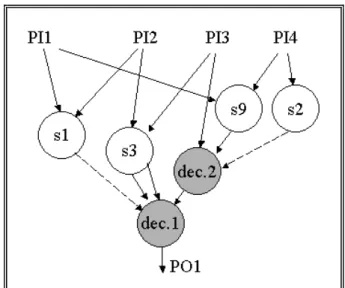
Then, the relation space will be extracted. The extraction of the relation space relies on data dependency analysis based on control data flow graph (CDFG). The CDFG of the HDL example in Figure2-5 is shown in Figure 2-7, where s denotes a statement and dec. represents a conditional statement or a decision.
Figure 2-7: Control Data Flow Graph (CDFG) of PO1
To obtain relation space of PO1 relies on a back trace from PO1 to the PIs according to the relationship in the data flow. In the back-tracing starting from PO1, the first traversed node is dec.1. dec.1 is added into the relation space. Then, because s6 is the statement on the taken branch of dec.1, s6 is the next traversed node. s6 is
also added in the relation space. The driving statements of s6 are dec.2 and s9 and the driving statements of dec.1 is s1. They are all added in the relation space, too. Similarly, the driving statements of dec.2 and s9 are found and added. Finally, the
relation space of PO1 are {dec.1, s6, s1, event1, dec.2, s9, s2, event2}. Therefore, the error space is {s1, s2, s6, s9, event1, dec.1, event2, dec.2}.
In additional to simple data dependency analysis of EPOs, Shi and et al further exploits the structure analysis and the nature of HDL operations to filter out more impossible error candidates [39]. A simple Verilog HDL code fragment shown in Figure 2-8 is used to illustrate how to apply the Rule I in [39] for error space reduction.
Figure 2-8: An example of applying Rule I in [39]
When an incorrect behavior is observed at PO1, if the error space identification approach in [46] is used, the back-tracing operation from PO1 on the CDFG will be the same as shown in Figure2-8(b). The resulted error space will be the same as the one shown in the upper part of Figure2-8(c).
However, when Rule I in [39] is applied, the authors state that the back-tracing from PO1 can stop at R1 by means of including the reversible path which contains a single reversible statement “PO2=~PO1” to the error space. This is because that R1 is on a reversible path to PO2. If R1 is incorrect, there must be some errors in the path from R1 to PO2 such that PO2 can have correct simulation value. As a result, the authors state that they can remove the statements “R1=A+B”, BTS(A), and BTS(B) and then add the reversible statement “PO2=~R1”. A reduced error space can be obtained by applying the Rule I. The resulted error space will be the one shown in the lower part of Figure2-8(c).
Besides Rule I, the authors also developed Rule II and III. Rule II states that given a HDL operation whose erroneous simulation value of left-hand variable and the correct value of left-hand variable are known, if there does not exist any values of other right-hand variables to produce the correct value of the left-hand variable while fixing the value of the target right-hand variable, the statement is incorrect or the simulation value of the target right-hand variable is incorrect. On the other hand, Rule III states that when the simulation value of one right-hand variable is a controlling value of the statement, the back-tracing from the other right-hand variables can be stopped. At least one erroneous statement requires to be retained in the error space.
The above works that focus on reducing number of error candidates are of course helpful for debugging faulty HDL designs. However, the size of the obtained error space can still vary from case to case. The number of error candidates may be plenty and searching true design errors in the obtained error space still requires much time.
Chapter 3
Observability Analysis on HDL
Descriptions for Effective Functional
Validation
3.1 Motivation
In functional validation, the simulation values of some signals of interest must be compared with their expected values to determine the consistency with the specification. The term observation points (OPs) is used to describe these signals because they act like observation windows to uncover bugs. Designers often select OPs according to their understanding of the specification and the availability of the expected values. However, erroneous effects caused by bugs are not always propagated to the assigned OPs. They may be masked while propagating to OPs. This situation prevents bug finding. Even worse, bugs may remain undiscovered through the manufacturing process if validation is not accurately gauged.
The Observability-based Code COverage Metric (OCCOM) is the first code coverage metric which considers the essential observability issue [18,19]. In their approach, the propagation of special tags that are attached to internal signals is simulated to predict the actual propagation of erroneous effects caused by design errors. Base on the likelihood that erroneous effects are propagated through each HDL
operation, the authors create tag simulation calculus and tag propagation rules to judge whether a tag can be propagated through an HDL operation or not.
However, the status of the tag propagation can only be propagated or un-propagated, providing only two levels of measurement; 1 and 0. However, the
error propagation is obviously not so certain and can be modeled by just propagated and un-propagated. Inevitably, erroneous effects with low observation opportunities may still be judged as propagated in some cases, thus giving overestimate the verification completeness. Even worse, mislead the verification resources to other portions of the DUV and let a design error remain undetected. We use the following example to illustrate this.
Consider a simple HDL example shown in Figure 3-1(a). Applying the input stimulus shown in Figure 3-1(b) to simulate the HDL code fragment in Figure 3-1(a), we can obtain the simulation results shown in Figure 3-1(c).
If we apply OCCOM to gauge the extent of the validation in the case shown in Figure 2-1, the tag propagation rule for “<” in [19] says that tag Δ and tag -Δ
injected on the signal counter can pass through statement 2 “if(counter<PI2)” and appear at PO1 at t=1 and t=5, respectively.
Consider a case that statement 7 carelessly written to be “counter=counter+2” by the circuit designer. The design error “counter=counter+2” in statement 7 causes an incorrect value 3 on counter at t=5, i.e. 3 is different from the correct value of counter 11. Because 3 is smaller than the correct value 11, the propagation of this
incorrect value 3 should be simulated by the -Δ injected on signal counter. We can
regard the incorrect value 3 as 11-Δ.
According to the tag propagation rules [18,19,43] for operation “<”, -Δ on
counter can be propagated through the operation “if(counter<PI2)” and makes the
output become 0+Δ . This implies that it is assumed that a decreasing value change is
very likely to change the evaluation result of “counter<PI2”, from FALSE to TRUE. However, we can see that the incorrect value 3 does not alter the evaluation result of “counter<PI2” as tag simulation calculus predicts. Tag simulation calculus fail to predict the error propagation in this example. In fact, in this example, the likelihood that a decreasing value change on counter is very unlikely to alter the evaluation result and to cause any erroneous effects on the output of “<”. We explain this fact by the below analysis.
Although in the above example we assumed that the design error “counter=counter+2” caused an incorrect value 3 at t=5, in practice, an incorrect value of counter can be any possible value that is different from the correct value 11. It can
be 0, 1, 2, 3, 4, 5, 6, 7, 8, 9, 10, 12, 13, 14, or 15. Among the 15 possible candidatess, the values {0~10} are smaller than the correct value 11 and each one of them can be can be regard as an individual 11-Δ. Because PI2 at t=5 is 2, only 1 and 0 can make
the evaluation result change from FALSE to TRUE. The other values {2~10} cannot, even if each of them is an erroneous value smaller than 11. Nine values ({2~10}) out of all possible fifteen incorrect values ({0~10},{12~15}) can not alter the output of “counter<PI2” to make the output result as 1+Δ. The likelihood that 11-Δ is
propagated through the operation “counter<PI2” should be quite low. Nevertheless, tag propagation rules did not actually take this likelihood into consideration and still assume that decreasing erroneous value change can be quite dramatic that it always change the evaluation result of “<”. Similar situations may also happen if tag propagation rules are used on some operations that may mask erroneous effects, such as “>”, “==”, “!=”, and “>>”.
In addition to inaccuracy, it is also unreasonable that tag propagation rules assume that erroneous values can never propagate through bit-select operations “[]” and “[:]”. In practice, erroneous effects of course can propagate through bit-select operations. Moreover, the assumed single tag model can only model the propagation behavior of exact one erroneous effect of a design error. If multiple design errors exist in the DUV, tag simulation calculus may not precisely determine whether the erroneous effects can be observed or not.
On the other hand, although Propagation Probability (PP) in PIE analysis is an accurate observability measure, its computation approach requires too much time as we’ve introduced in section 2.2. Therefore, we intend to develop a new Probabilistic
Observability Measures (POM), which are more accurate than tag-based observability measures and require much less computation time than PP. There are some possible applications for our proposed POM.
A new observability-based code coverage metric – In our new
observability-based code coverage metric, a statement is considered as covered if it is first exercised and the observability of the statement’s output variable is high enough. This is similar to the well-known fault simulation that requires fault activation and propagation.
Indicating hard-to-observe points – If some signals are less likely to be observed,
bugs may hide behind these points and become very difficult to reveal via limited observation points. It does not mean that behind these signals there must be some design errors, but it provides where the input stimuli does not suitably verify with both exercitation and observability considerations. By using our observability analysis, designers can designate candidates for assertion insertion to prevent potential bugs from hiding. This can increase the verification efficiency, too.
3.2 Probabilistic Observability Measure for HDL
Descriptions
Despite completion of a successful simulation in which the simulated values of all the Observation Points (OPs) consistent with the correct values, it is still possible that some incorrect values existed at some time instances but remain hidden due to the
error masking. Assuming that the simulation values of all the OPs are consistent with
the expected values, the goal of our work is to analyze which signals will most likely have incorrect values hiding at which time instances. This prevents overestimating validation completeness and can point out hard-to-observe points during the previous phases of simulation for leading verification resources to those weak points. In the section, we introduce how we model the error masking and define Probabilistic Observability Measure (POM).
3.2.1 Control Data Flow Graph
The Design Under Validation (DUV) is modeled as a modified Control/Data Flow Graph (CDFG) G = (V, E), where V is the set of vertices and E is the set of edges connecting vertices. In order to explain the CDFG more clearly, the CDFG appearing in Figure 3-2 is used as an example of the HDL code shown in Figure 3-1. Let v be a vertex in V. Each vertex v corresponds to an operation in the HDL code. Function fv and variable yv are also associated with vertex v. Function fv is the function of the operation that v corresponds to. Variable yv is the output variable of fv or the
corresponds to the operation “a=PI1*4” at line 1 in the HDL code. Function f1:* is multiplication “*” and y1:* is signal a. Vertex “2:if” corresponds to the operation “if(…) … else ...” in lines 2 to 4 of the HDL code, and its functionality is quite similar to a multiplexer. Vertex PO1 is a special vertex representing the primary output PO1 in the circuit. An edge (v, u) ∈E indicates that the input of vertex u is data dependent on the output of v. As shown in Figure 3-2, an edge (1:*, 4:=) exists since the operation “4:=” takes the output of vertex “1:*” as its input. The fanout of v is a set of vertices u such that there is an edge from v to u. Similarly, the fanin of v is a set of vertices k such that there is an edge from k to v. A path from vertex u to vertex u’ is a sequence <v0, v1, v2,…, vk> of vertices such that u = v0, u’ = vk, and (vi-1, vi) ∈ E.
Figure 3-2: The CDFG of the HDL code in Figure3-1
3.2.2 Masked Value Set and Probabilistic Observability Measure
If a single incorrect value w ever existed on the output variable of vertex v yv at time instance t=ti in the design under validation during simulation, this incorrect value
of clock1. If not, the simulation phase is not successful. More specifically, the simulated value of an observation point OPj at an arbitrary positive edge of clock t=ck must be the same as the correct value. The incorrect value w must be masked by some vertices on the paths from vertex v at t=ti (denoted as v@t=ti) to observation point OPj at t=ck (denoted as OPj@t=ck). In the following descriptions, “v at t=ti” and “v in time frame t=ti” will be used in turn. A formal description of error masking is given in (3.1).
)
@
(
)
(
@ @t t OP t c j k vw
CV
OP
t
c
f
k j i→ ==
=
= (3.1)where
f
v@t=ti→OPj@t=ck is the function of the paths from v in time frame t=ti to OPjin time frame t=ck and CV(OPj@t=ck) is the correct value of OPj at t=ck.
If there are m total observation points {OP1,OP2,…,OPm} and o clock cycles in
the simulation phase, w must be masked on its way to all the observation points in all time frames such that it is not uncovered during the entire simulation process. For each observation point OPj in each time frame t=ck, the function of the paths from
vertex v in time frame t=ti that go to OPj at t=ck must generate the correct value of
OPj at t=ck with this incorrect value w as described in (3.2).
II
jm ko fv t ti OPj t ck w CV OPj t ck 1 1 @ @ ( ) ( @ ) = = = → = = = (3.2)1 We assume that the simulation values of all the observation points are compared with the correct
values only on the positive edges of clock signal. If the design under validation is a falling-edge-triggered or double-edge-triggered design, the assumption along with the modeling and the computation can easily be changed to fit to it.
The set of all possible values of vertex v’s output that can satisfy (3.2) is defined as the Masked Value Set (MVS) of vertex v at time instance t=ti (MVS(v@t=ti)). A
more formal definition is given in (3.3). Each element in MVS(v@t=ti) retains the
correct values of all the observation points at all positive edges during simulation.
} ) @ ( ) ( | { ) @ ( 1 1 @ @
II
m j o k k j c t OP t t v i x f x CV OP t c t t v MVS k j i = = = → = = = = = (3.3)The correct value of the output of vertex v at t=ti is in MVS(v@t=ti) and this can
justify the existence of MVS(v@t=ti). If MVS(v@t=ti) has only one element, this
element must be the correct value and no error masking can occur. On the other hand, if the set contains many elements, there will be many elements other than the correct values2 in the set. An incorrect value caused by some bugs may very possibly be one of these elements and thus be masked. (The incorrect value can also be outside the set such that it is revealed.) The more elements in MVS(v@t=ti), the more likely the
simulation value of v is one of these masked incorrect values. Hence, the Likelihood Of Error Masking (LOEM) of v at t=ti is defined as (3.4).
1 2 1 | ) @ ( | ) @ ( − − = = = BW i i t t v MVS t t v LOEM (3.4) v y BWis thebit width of
where
, . Its complement is the observability measure of v at
t=ti, as described in (3.5). 1 2 1 | ) @ ( | 1 ) @ ( − − = − = = BW i i t t v MVS t t v ity Observabil (3.5)
2 Although the elements other than incorrect value in the Masked Value Set of v at t=t
i are not all
masked incorrect values, some of them may be don’t care values of v at t=ti. However, the
3.3 Observability Computation Algorithm
Our observability computation algorithm is a topology-based analysis with time
frame expansion to handle the sequential behavior of the DUV. While calculating the
observability of the output variable of vertex v in time frame t=ti, the algorithm will
consider each sensitized path from v in time frame t=ti that goes to any observation
point in each time frame. The path-oriented computation scheme is defined in (3.6), which can be transformed from (3.3).
II
jm ko v t t OP t c j k i x f x CV OP t c t t v MVS k j i 1 1 @ @ ( ) ( @ } | { ) @ ( = = = → = = = = = (3.6) The set {x | f @ @ (x) k j i OP t c t tv = → = =CV(OPj@t=ck)} is defined as the Masked Value
Set of vertex v at time instance t=ti with respect to OPj at t=ck (denoted as
MVS(v@t=ti)OPj@t=ck). An element of the set other than the correct value can be regarded as an incorrect value that is masked by some vertices on the paths from v at
t=ti to OPj at t=ck, thus keeping the correct value of OPj at t=ck.
According to (3.6), if it is possible to derive MVS(v@t=ti)OPj@t=ck for each observation point OPj at each time frame t=ck, then intersecting these sets produces
MVS(v@t=ti). If there is exactly one path from v at t=ti to an observation point OPj at
t=ck, an induction-based computation approach is proposed to compute exact
MVS(v@t=ti)OPj@t=ck, which is introduced in section 3.3.1 and 3.3.2. If there are multiple paths from v at t=ti to OPj at t=ck, a quick estimation approach that
in section 3.3.3. Section 3.3.5 introduces the entire algorithm incorporating both of them and section 3.3.4 discusses time-saving strategies.
3.3.1 MVS Computation for Single Path
Assume that there is a sensitized path P from a vertex b at time instance t=ti to
an observation point OPj at a positive edge of clock t=ck. As an example, one such
path <b@t=ti, an, an-1,…, a2, a1, OPj@t=ck> is shown in Figure3-3 and will be used in
the following explanations. For the case of a single path, we develop an algorithm to compute MVS(b@t=ti)OPj@t=ck as shown in the pseudo code in Figure3-4.
Figure 3-3: A Path from b@t=ti to OPj@t=ck
For each observation point at each positive clock edge, the algorithm will recursively call subroutine MVS_for_vertex to perform MVS computation and use a Depth First Search (DFS) strategy for backward traversals. The input of the subroutine is a previously computed set of integers (PreviousMVS), the currently traversed vertex v, and the current time frame ti. If the currently traversed vertex v is a
![Table 2-4: Tag calculus for ADD (+) Operation in [18,19]](https://thumb-ap.123doks.com/thumbv2/9libinfo/8624789.191813/27.892.187.711.956.1085/table-tag-calculus-for-add-operation-in.webp)
![Figure 2-8: An example of applying Rule I in [39]](https://thumb-ap.123doks.com/thumbv2/9libinfo/8624789.191813/36.892.133.755.452.871/figure-example-applying-rule-i.webp)
