用無母數迴歸方法監控隨機效應曲線型品質特性之製程

國 立 交 通 大 學

統計學研究所

碩 士 論 文

用無母數迴歸方法監控隨機效應曲線型品質特性

之製程

Monitoring Random Effect Profiles by Nonparametric

Regression

研 究 生 ： 蔡明曄

指導教授 ： 洪志真 博士

用無母數迴歸方法監控隨機效應曲線型品質特性

之製程

Monitoring Random Effect Profiles by Nonparametric

Regression

研 究 生：蔡明曄

Student： Ming-Ye Tsai

指導教授：洪志真

Advisor： Dr. Jyh-Jen Horng Shiau

國 立 交 通 大 學

統計學研究所

碩 士 論 文

A Thesis

Submitted to Institute of Statistics

College of Science

National Chiao Tung University

in Partial Fulfillment of the Requirements

for the Degree of

Master

in

Statistics

June 2006

Hsinchu, Taiwan, Republic of China

用無母數迴歸方法監控隨機效應曲線型品質特性

之製程

研究生： 蔡明曄 指導教授： 洪志真 博士

國立交通大學統計學研究所

摘要

監控製程與產品之曲線型資料在統計品質管制中是ㄧ個非常熱門且

有前景的研究領域。我們的研究將以對具有隨機效應之非線性曲線型資

料的監控方法為主。

對隨機效應模式，我們利用主成分分析來分析曲線型資料的共變異

結構，並利用每個曲線型資料所得之主成分分量來做監控。在第二階段

中，因為個別的主成分分量很難區別開變動的趨勢，所以我們建議利用

combined chart，即合併主成分分量的方法來做監控。

在第一階段中，因為主成分分量的相依特性，我們採用

圖來檢測

穩定性。我們利用大量模擬的方法來說明，當 outliers 出現的形式是短

暫時，

T 表現的較

T 佳。

而且，我們也發現用來建造控制圖的主成分個數會影響偵測力。我

們採用交互驗證(cross-validation)的方法，來選擇主成分的個數。

Monitoring Random Effect Profiles by

Nonparametric Regression

Student： Ming-Ye Tsai Advisor： Dr. Jyh-Jen Horng Shiau

Institute of Statistic

National Chiao Tung University

ABSTRACT

The monitoring of process and product profiles is a very popular and

promising area of research in statistical process control. This study is aimed

at the monitoring scheme for nonlinear profiles with random effects.

For random effect models, we use the technique of principal component

analysis to analyze the covariance structure of the profiles and use principal

component scores of each profile to perform monitoring. In Phase II, since it

is difficult for each principal component score to have identified direction of

shifts, we recommend using a combined chart scheme that combines the

principal component scores to perform monitoring.

In the historical analysis of Phase I data, due to the dependency of

principal component scores, we adopt the

T chart to check for stability.

We show by simulation that the sample-covariance-based

T performs

better than the successive-difference-based

T for temporal shifts.

Also, the number of principal component scores used in constructing

control charts has an effect on the detecting power. We adopt the

cross-validation to choose the number of principal component scores.

誌 謝

Contents

abstract (in Chinese) i

abstract (in English) ii

acknowledgement (in Chinese) iii

contents iv

list of tables vi

list of figures viii

1 Introduction 1

2 Literature Review 4

3 Methodologies 7

3.1 Procedures . . . 7

3.2 B-Splines . . . 9

3.3 Principal Component Analysis . . . 11

3.4 A Simple Cross-Validation Procedure . . . 16

3.5 T2 _{statistics . . . 17}

4 Simulation Studies - Aspartame Example 18 4.1 Settings for Simulation . . . 18

4.2 Number of Principal Components . . . 19

4.3 Phase I monitoring . . . 20

4.4 Phase II monitoring . . . 23

5 A Case Study - VDP Example 28 5.1 Phase I monitoring . . . 28

6 Conclusions 30

List of Tables

1 The performance assessed by detecting power and false-alarm rate for T2

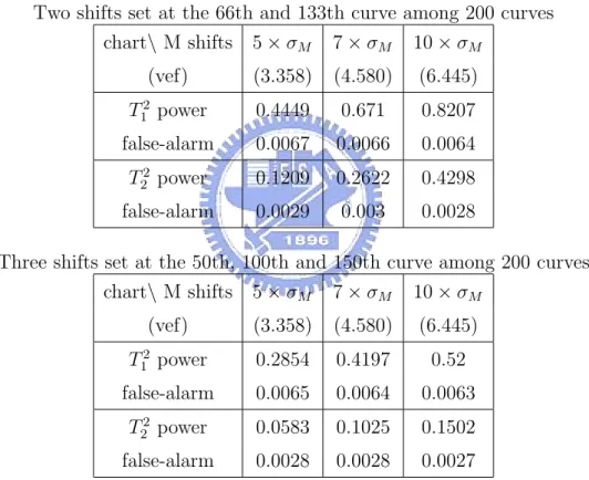
1 and T22 to detect I shifts with temporal shifts. . . . 34

2 The performance assessed by detecting power and the false-alarm rate for T2 1 and T22 to detect M shifts with temporal shifts. . . 35

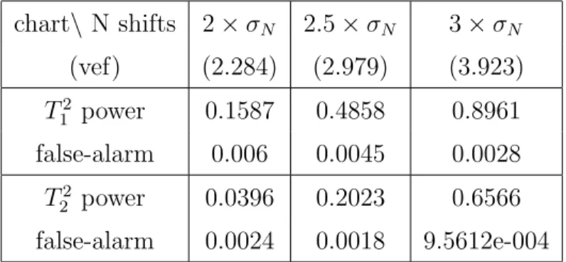
3 The performance assessed by detecting power and the false-alarm rate for T2 1 and T22 to detect N shifts with temporal shifts. . . 36

4 ARL comparison for I-shift (µI = 1 + 0.2 × α). . . 37

5 ARL comparison for M-shift (µM = 15 + 1 × β). . . 38

6 ARL comparison for N-shift (µN = −1.5 + 0.3 × γ). . . 39

7 Real ARL comparison for I-shift (µI = 1 + 0.2 × α). . . 40

8 Real ARL comparison for M-shift (µM = 15 + 1 × β). . . 40

9 Real ARL comparison for N-shift (µN = −1.5 + 0.3 × γ). . . . 41

10 Combined chart ARL for I-shift (µI = 1 + 0.2 × α). . . 41

11 Combined chart ARL for M-shift (µM = 15 + 1 × β). . . 42

12 Combined chart ARL for N-shift (µN = −1.5 + 0.3 × γ). . . . 42

13 Real combined chart ARL for I-shift (µI = 1 + 0.2 × α). . . . 43

14 Real combined chart ARL for M-shift (µM = 15 + 1 × β). . . 43

15 Real combined chart ARL for N-shift (µN = −1.5 + 0.3 × γ). . 43

16 ARL comparison for simultaneous I(row) and M(column) shifts. 44 17 ARL comparison for simultaneous I(row) and N(column) shifts. 45 18 ARL comparison for simultaneous M(row) and N(column) shifts. . . 46

19 ARL comparison for I-shift in variance. . . 47

20 ARL comparison for M-shift in variance. . . 48

22 ARL comparison for shifts in principal component 1. . . 50 23 ARL comparison for shifts in principal component 2. . . 51

List of Figures

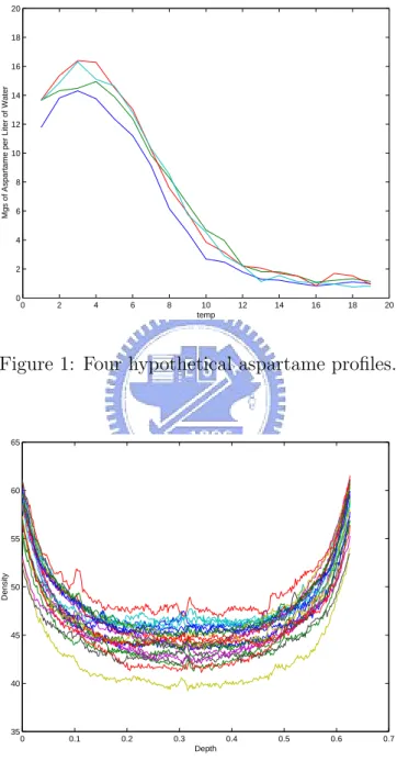
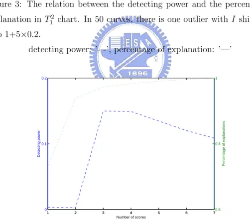
1 Four hypothetical aspartame profiles. . . 52 2 Original 24 VDP–profiles. . . 52 3 The relation between the detecting power and the percentage

of explanation in T2

1 chart. In 50 curves, there is one outlier

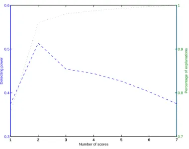
with I shift from 1 to 1+5×0.2. . . 53 4 The relation between the detecting power and the percentage

of explanation in T2

2 chart. In 50 curves, there is one outlier

with I shift from 1 to 1+5×0.2. . . 53 5 The relation between the detecting power and the percentage

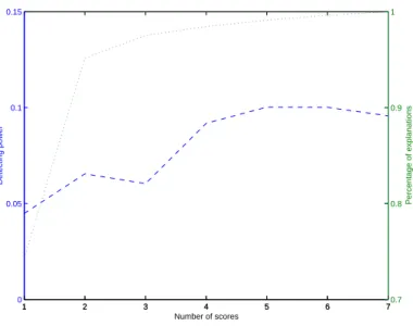
of explanation in T2

1 chart. In 50 curves, there are two outliers

with M shift from 15 to 15+5×1. . . 54 6 The relation between the detecting power and the percentage

of explanation in T2

2 chart. In 50 curves, there are two outliers

with M shift from 15 to 15+5×1. . . 54 7 The relation between the detecting power and the

percent-age of explanation in T2

1 chart. In 50 curves, there are three

outliers with N shift from -1.5 to -1.5+2×0.3. . . 55 8 The relation between the detecting power and the

percent-age of explanation in T2

2 chart. In 50 curves, there are three

outliers with N shift from -1.5 to -1.5+2×0.3. . . 55 9 The cross-validation results for one outlier with a shift of five

sigma in I among fifty profiles. . . 56 10 The cross-validation results for two outliers with a shift of five

sigma in M among fifty profiles. . . 56 11 The cross-validation results for three outliers with a shift of

two sigma in N among fifty profiles. . . 57 12 The resulting histogram for two-fold cross-validation. . . 57

13 The resulting histogram for ten-fold cross-validation. . . 58

14 The resulting histogram for delete-one cross-validation. . . 58

15 Original 200 aspartame profiles. . . 59

16 Fitted B-splines with d.f.=5 . . . 59

17 T2 1 control chart. . . 60

18 T2 2 control chart. . . 60

19 T2 1 control chart after the out-of-control profile was removed. . 61

20 T2 2 control chart after the out-of-control profile was removed. . 61

21 Shifts in I. . . 62

22 Shifts in M. . . 62

23 Shifts in N. . . 63

24 First four eigenvectors. . . 63

25 Principal component 1. . . 64

26 Principal component 2. . . 64

27 Principal component 3. . . 65

28 Principal component 4. . . 65

29 ARL comparison for I shifts in mean. . . 66

30 ARL comparison for M shifts in mean. . . 66

31 ARL comparison for N shifts in mean. . . 67

32 ARL comparison for I shifts in variance. . . 67

33 ARL comparison for M shifts in variance. . . 68

34 ARL comparison for N shifts in variance. . . 68

35 ARL comparison for mean shifts and variance shifts for the combined chart. . . 69

36 Fitted B-splines with d.f.=16. . . 70

37 Principal component 1. . . 70

38 Principal component 2. . . 71

39 Principal component 3. . . 71

41 First four eigenvectors. . . 72 42 T2 1 control chart. . . 73 43 T2 2 control chart. . . 73 44 Simulated 24 VDP–profiles. . . 74 45 Comparison of the real mean profile and the mean profile

es-timate of the simulated data. . . 74 46 Comparison of the real profiles and the simulated profiles for

the first eigenvector. . . 75 47 Comparison of the real profiles and the simulated profiles for

the second eigenvector. . . 75 48 Comparison of the real profiles and the simulated profiles for

the third eigenvector. . . 76 49 Comparison of the real profiles and the simulated profiles for

the fourth eigenvector. . . 76 50 Comparison of the real eigenvalues and the simulated ones. . . 77

1

Introduction

Statistical process control (SPC) has been widely applied in many areas, espe-cially in industries. Classical methods for SPC assume that the quality of the product or process can be measured by one or multiple quality characteristics. However in many situations, the response of interest is not a single variable but rather a function of some independent variables. This functional response is called a profile. An example of profiles is the dissolving process of aspar-tame, an artificial sweetener, which is characterized by the amount of that dissolves per liter of water at different levels of temperature; see Kang and Albin (2000). For illustration, Figure 1 shows the plot of four hypothetical aspartame profiles. Another example mentioned in Kang and Albin (2000) is a semiconductor manufacturing problem that occurs during the etching step. In this example, the calibration of a mass flow controller in which the performance of the process is characterized by a linear function; see Mestek et al. (1994). There is also an interesting example introduced by Walker and Wright (2002), called vertical density profiles (VDP). The density is mea-sured using a profilometer that uses a laser device to take measurements at fixed depths across the thickness of the engineered wood board. As an illus-tration, Figure 2 shows the VDP data from Walker and Wright (2002). The data set is available at http://bus.utk.edu/stat/walker/VDP/Allstack.TXT. The authors proposed a method using additive models to assess the sources of variation in the density profiles of particleboards.

Kang and Albin (2000) studied the problem of linear profile monitoring. Let the output of a process be a random variable Y which depends linearly on an independent variable X. They modeled the profiles by the simple lin-ear regression model, Y = A0+ A1X + ², Xl ≤ X ≤ Xh, where A0 and A1

are parameters and Xl and Xh define the range of X in which the process

and normally distributed with mean 0 and variance σ2_{. They proposed two}

approaches to monitoring profile data: (i) monitoring the parameters, the intercept (A0) and slope (A1), simultaneously with the Hotelling T2 chart

and (ii) using the regular EWMA and R charts for profile monitoring by treating the residuals of the sample line to the in-control reference line as a rational subgroup. Kim et al. (2003) proposed another approach called

EW MA3, which they showed was comparable to the approach of Kang and

Albin (2000). They centered the X-values to make the least squares esti-mators of the Y-intercept and slope independent of each other. So that the intercept and slope can be monitored separately. They constructed three EWMA charts to monitor intercept, slope, and the variation, separately.

Shiau and Weng (2004) extended the above profile monitoring scheme to a scheme for more general profiles. No assumption are made for the form of the profiles except the smoothness. The nonparametric regression model con-sidered is Y = g(x) + ², where g(x) is a smooth function and ² is the random error as before. Spline regression was adopted as the curve fitting/smoothing technique. They proposed an EWMA chart for detecting the mean shifts, an R chart for variation changes, and an exponentially weighted moving stan-dard deviation (EWMSD) chart for the variation increase.

Note that the models described so far are a deterministic line/curve plus random noises. In this paper, based on Shiau and Weng (2004), we extend the fixed effect model to a random effect model in order to provide more variability that we often observe in many profile data, e.g., the aspartame example and VDP example. We use the function Y = I + MeN (x−1)2

+ ² given in Shiau and Weng (2004) as our illustrative example, where I, M, N are considered to be random variables. Like Shiau and Weng (2004), we use the B-spline regression technique to smooth profiles. With the random effect model, we put emphasis on the covariance structure. To analyze the

covariance matrix, it is natural to consider the technique of the principal component analysis (PCA).

The PCA is very useful in summarizing and interpreting a set of profile data with the same equally spaced values of the independent variable X for each profile. Castro et al. (1986) showed that the principal modes of variation consist of eigenfunctions of the process covariance function and gave procedures for estimating these eigenfunctions from a set of observed curves. Rice and Silverman (1991) proposed a method for estimating the mean function nonparametrically under the assumption that it is smooth. They also suggested a variant of the usual cross-validation for choosing the degree of smoothing to be employed. And in the estimation of covariance structure, they primarily concerned with the first few eigenfunctions that were smoothed and the eigenvalues that decayed rapidly. Jones and Rice (1992) suggested that a simple PCA be used to identify important modes of variation among the curves and that the principal component scores be used to identify particular curves which clearly demonstrate the form and extent of a particular mode of variation.

In this paper, we construct our monitoring schemes by utilizing the eigen-vectors and principal component scores obtained from PCA. If these scores corresponds to separate modes of variation, then it is natural to monitor each principal component score for what it represents. If not, we suggest a combined-chart scheme that combines the charts of these principal compo-nent scores for profile monitoring. Finally, a simulation study is conducted to evaluate the performance of each principal-component-score chart and the combined-chart in terms of the average run length (ARL). The simulation study demonstrates that the combined chart scheme is comparable with the best principal-component-score chart.

T2 _{statistics, T}2

1 and T22, in which different covariance estimators are used.

Also, it is found from the study that the number of principal component scores used in constructing T2 _{statistics affects the power of detecting}

out-of-control profiles significantly. In this study, we use the cross-validation method, one of the most popular procedures for model selection, to choose the number of principal component scores.

Section 2 reviews the methods proposed by Shiau and Weng (2004) and Shiau and Lin (1999) in which a set of degradation paths was modeled by a stochastic process and PCA was employed to analyze the covariance struc-ture. Section 3 describes some methodologies used in this paper, including the B-spline regression technique, principal component analysis, procedure of cross-validation, and the proposed control schemes in details. Section 4 presents the simulation results of Phase II monitoring with some discussions along with some recommendations for Phase I monitoring. Section 5 presents a case study using the VDP data from Walker and Wright (2002). Finally, Section 6 concludes the paper with a brief summary and some remarks.

2

Literature Review

Shiau and Weng (2004) proposed a profile monitoring scheme for profiles of flexible shape. Unlike the combined EWMA/R chart proposed by Kang and Albin (2000), they recommended using the EWMA to monitor the residual average for detecting mean shifts and the R chart to monitor the residual range for detecting standard deviation shifts of the residuals individually in order to have better detecting power. Also, they proposed an EWMSD control chart to detect shifts in process variation.

In Shiau and Weng (2004), an exponential profile of the form Y = I +

Me−N (x−1)2

showed by simulation studies that, for I, M, and N shifts in the exponential profile, the EWMA chart performed well in detecting shifts. And for standard deviation shifts, the EWMSD chart is a good choice while one can also use the R chart. Also, they showed that, for the linear profile example given in Kang and Albin (2000), their methods were slightly effective than the methods of Kang and Albin (2000) and Kim et al. (2003).

Shiau and Lin (1999) proposed a nonparametric regression accelerated life-stress (NPRALS) model to analyze the accelerated degradation tests (ADT) data. In order to model a set of degradation paths by a stochas-tic process, they made the following assumptions:

1. The sample degradation path of each experimental subject is a realiza-tion of an underlying stochastic process {X(t), t ∈ T }, where T is an interval.

2. The model for X(t) is

X(t) = µ(t) + ω(t) + ²(t), (1)

where µ(t) ≡ E[X(t)], ω(t) ≡ a stochastic process with mean 0 and covariance function r(s, t)≡Cov[ω(t), ω(s)], and

²(t) ≡ uncorrelated error terms with E[²(t)]=0 and V ar[²(t)]=σ2_.

3. The acceleration stress affects only the degradation rate, not the shape of the degradation curve.

With these assumptions, they used µ(t) to denote the mean curve under the normal condition (un-accelerated) and µ(a·t) to denote the accelerated mean curve where a is the acceleration factor and usually a > 1.

In their model, there are m stress levels in the experiments. And for stress level i, there are ni experimental units. Also, t1, . . . , tp are the measured

points of the product characteristic for each experimental unit. By using the functional principal component technique, they model the ADT data by

Xi,j,k = µ(ai· tk) +

L

X

q=1

²i,j,q · ρi,q(tk), (2)

where 1 ≤ i ≤ m, 1 ≤ j ≤ ni, 1 ≤ k ≤ p, 1 ≤ q ≤ L, and L is a positive

integer no more then p. So the random component ω(t) + ²(t) of equation (1) is then replaced by a random combination of functional principal compo-nents {ρi,q(·), q = 1, . . . , L}. And they provided an iterative algorithm to

estimating µ(·) and a1, . . . , am.

Also, they investigated the covariance structure of X(·). First, for i = 1, . . . , m, compute (Vi)s,r = 1 ni− 1 · ni X j=1 [Xi,j,s− ˆµi(ts)] · [Xi,j,r − ˆµi(tr)]

for 1 ≤ s, r ≤ p, where ˆµ(·) is the estimate of µ(·). Let ˆρ_i,q ≡ (ˆρi,q(t1), . . . ,

ˆ

ρi,q(tp))0 be the eigenvector corresponding to the q-th largest eigenvalue λi,q

of Vi, where i = 1, . . . , m and q = 1, . . . , p. Then estimate:

• σ2

i,q by λi,q.

• ρi,q(·) by smoothing {ˆρi,q(tk), k = 1, . . . , p} on {tk, k = 1, . . . , p}.

At the end of the paper, they presented a real data analysis with their NPRALS model. Also, in order to show how well their procedure does in recovering the truth, they conducted a simulation study. They simulated the degradation data curves by using equation (2). Treat ˆµ(·), λi,q, and

the smoothed {ˆρi,q(tk), k = 1, . . . , p} obtained from the previous real data

analysis as the true values of µ(·), σ2

i,q, and ρi,q(·), respectively. The following

• Compute: (Vi)s,r = 1 ni · ni X j=1 [Xi,j,s− µi(ts)] · [Xi,j,r− µi(tr)] for 1 ≤ i ≤ m, 1 ≤ j ≤ ni, 1 ≤ k, s, r ≤ p.

• Generate ²i,j,q from N(0, σ2i,q), 1 ≤ j ≤ ni, 1 ≤ q ≤ L.

• Generate: ˜ Xi,j,k = µi(tk) + L X q=1 ²i,j,q· ρi,q(tk) for 1 ≤ j ≤ ni, 1 ≤ k ≤ p.

By simulation, they showed that their NPRALS model performed very well in recovering the features of the original degradation data curves.

3

Methodologies

3.1

Procedures

In this paper, as an illustrative example, we use the model

Y = I + MeN (x−1)2

+ ²

where I ∼ N(1, 0.22_{), M ∼ N(15, 1), N ∼ N(−1.5, 0.3}2_{) , ² ∼ N(0, 0.3}2_),

and x=0.64, 0.8, . . ., 3.52 to simulate the profile data of the aspartame example. We generate 200 profiles to serve as our historical data for Phase I analysis.

We apply the B-spline smoothing technique to filter out the noise. For the model X(t) = µ(t) + W (t) + ²(t), this is to filter out ²(t) so that the actual signals can be better extracted from the data. These extracted signals will be smoother and can explain the variation among profiles better. As

the variance of ²(t) tends larger, the advantage of smoothing tends more profound.

In Phase I monitoring, first we select the number of principal component (PC) scores to be used by cross-validation and then use the T2 _statistics

of the score vectors to detect the outliers. The details of these methods are given in Subsections 3.4 and 3.5. This procedure will continue until, all the remaining profiles are within the control limit. Then we can apply the technique of PCA to these ”in-control” profiles and the principal components obtained will be used for the Phase II monitoring.

We summarize the whole simulation procedure as follows:

• Generate historical profile data at set points x=0.64, 0.8, . . ., 3.52 by y = I + MeN (x−1)2

+ ²,

where I ∼ N(1, 0.22_{), M ∼ N(15, 1), N ∼ N(−1.5, 0.3}2_{) , and ² ∼}

N(0, 0.32_).

• Smooth each of the discrete profile data with the B-spline smoothing

technique.

• Select the number of effective principal components by the

cross-valida-tion method.

• Phase I: use T2 _{statistics to remove outliers until the remaining profiles}

are all in control. Then, use PCA to obtain important features, by which the in-control process is characterized.

• Phase II: We compute PC scores for each of the incoming profiles.

And use the independent property of the scores to check the stability of the incoming profile by monitoring each score separately or by the combined-chart scheme.

3.2

B-Splines

One basic objective of the data analysis is to identify the signals in a set of data. But this gets complicated with the existence of random noise in the data. That is, the goal is to filter out the random noise from the data in order to get the signal. In order to extend nonlinear profiles of a fixed form to smooth profiles of any shapes, a smoothing technique is needed for de-noising sample profiles. The idea of smoothing is to fit a flexible function whose final form is determined by the data and by the chosen level of smoothness of the curve. That is, let the data speak for themselves. One popular way is to fit noisy data by splines. Frequently, cubic splines−piecewise cubic polynomials with continuous second derivatives−are used for such approximation.

Consider the following nonparametric regression model:

yi = g(xi) + ²i, i = 1, . . . , p, (3)

where g(x) is a smooth regression curve and ²i’s are i.i.d. Gaussian variables

with zero mean and common variance σ2 _{> 0 . In this paper, to estimate g(x),}

we adopt the B-spline regression method for its popularity and simplicity. Simply put, the B-spline regression is just a multiple linear regression with B-spline bases.

Before we go on, we first give a brief description on B-spline bases. Details can be found in de Boor (1978). Let b denote the number of bases and k be the order of the B-splines. Note that the degree of the polynomials is k − 1, hence each basis of order k is a k −2 continuously differentiable function. For example, k = 4 for cubic splines. Also let the interval [u, v] be the domain of interest. For spline smoothing, knots are the points where the higher-order derivatives could be discontinuous. For b bases, we need b + k knots, denoted by t1, . . . , tb+k, such that tk = u and tb+1 = v. And let Bl,k denotes the l-th

by Bl,1(t) =    1 for tl≤ t < tl+1, 0 for t < tl or t ≥ tl+1. For k ≥ 2, Bl,k(t) = t − tl tl+k−1− tl Bl,k−1(t) + tl+k− t tl+k − tl+1 Bl+1,k−1(t).

Note that Bl,k is nonzero only on the interval (tl, tl+k). A B-spline of order

k can then be constructed as g(x) =

b

X

l=1

clBl,k(x), for x ∈ [u, v],

where cl’s are the unknown B-spline coefficients to be estimated from data.

For the B-spline regression, the nonparametric regression model in equa-tion (3) can then be replaced by the following linear model:

yi = b

X

l=1

clBl,k(xi) + ²i, i = 1, . . . , p. (4)

Given a set of data, {(xi, yi), i = 1, . . . , p}, the spline regression method finds

the best spline approximation via the following least squares problem:

min c p X i=1 {yi− b X l=1 clBl,k(xi)}2, (5)

where c = (c1, . . . , cb)0. Then the least squares estimator of c is

ˆ

c = (B0_B)−1_B0_{y, (6)}

where y = (y1, . . . , yp)0, ˆc = (ˆc1, . . . , ˆcb)0, and B is the p × b design matrix

with the (i, l)-th element Bl,k(xi), l = 1, . . . , b, i = 1, . . . , p. Under the model

in equation (4), ˆc has a multivariate normal distribution with mean vector c and variance-covariance matrix Σ = σ2_(B0_B)−1_.

Note that the number of bases b acts as the smoothing parameter in nonparametric regression and it is well known that the choice of the smooth-ing parameter is crucial in nonparametric regression estimation. Also, the

boundary effect inherited in most of the smoothing methods is another issue of concern.

3.3

Principal Component Analysis

The following materials on PCA are taken from Anderson (2003). PCA is a multivariate procedure that rotates the data such that maximum variabil-ities are projected onto the axes. Essentially, a set of correlated variables are transformed into a set of uncorrelated variables ordered by the amount of variation explained. Then these uncorrelated variables, called principal components, are linear combinations of the original variables, and the last of these variables can be removed with minimum loss of information contained in data. The main usage of PCA is to reduce the dimensionality of a data set while retaining as much information as possible.

Principal components have special properties or features in terms of vari-ance. They turn out to be the characteristic vectors of the covariance matrix. Suppose the random vector Y of p-components has covariance matrix Σ. Since we are only interested in the covariance matrix Σ, without loss of gen-erality, we may assume that the mean vector is 0. Let β be a p-component column vector such that β0_{β = 1. The variance of β}0_{Y is}

E(β0Y)2 _{= E(β}0_YY0_{β) = β}0_E(YY0_{)β = β}0_{Σβ , (7)}

where E denotes the expectation. In order to determine β0Y with the max-imum variance subjected to β0_{β = 1, let}

φ = β0Σβ − λ(β0β − 1) , (8) where λ is a Lagrange multiplier. Then the partial derivatives of φ with respect to β is

∂φ

since β0_{Σβ and β}0_{β have derivatives everywhere in the region that contains}

β0_{β = 1. Thus, set}

∂φ

∂β = 2Σβ − 2λβ = 2(Σ − λI)β = 0 . (10)

In order to get the solution of equation (10) with β0β = 1, we must have

Σ − λI singular. In other words,

|Σ − λI| = 0 . (11)

Since |Σ − λI| is a polynomial in λ of degree p, thus equation (11) has p roots. Without loss of generality, let λ1 ≥ λ2 ≥ · · · ≥ λp . Then

β0_{Σβ = λβ}0_{β = λ . (12)}

This shows us that if β satisfies equation (10) and β0β = 1, then the variance

of β0Y is λ.

Let β(1) _{be a normalized solution of (Σ−λ}

1I)β = 0. Then β(1)is the

cor-responding first principal component vector and U1 = β(1) 0

Y is a normalized linear combination of the original variables with maximum variance. Next, we want to find a normalized linear combination β0_{Y that has maximum}

variance of all linear combination uncorrelated to U1. That is,

0 = E(β0YU0

1) = E(β0YY0β(1)) = β0E(YY0)β(1) = β0Σβ(1) = λ1β0β(1) ,(13)

since Σβ(1) _{= λ}

1β(1). So now, we want to maximize

φ2 = β0Σβ − λ(β0β − 1) − 2ν1β0Σβ(1) , (14)

where λ and ν1 are both Lagrange multipliers. Then the partial derivatives

of φ2 is

∂φ2

∂β = 2Σβ − 2λβ − 2ν1Σβ

Multiply β(1)0

on the left of the above equation, then set it to zero. We have

0 = 2β(1)0 Σβ − 2λβ(1)0 β − 2ν1β(1) 0 Σβ(1) _{= −2ν} 1λ1 . (16)

Thus, ν1 = 0 and β must satisfy equation (10), and therefore λ must satisfy

equation (11). Let λ(2) be the maximum of λ1, . . . , λp such that there is a

vector β satisfying (Σ − λ(2)I)β = 0, β0β = 1, and equation (13). We denote

this vector by β(2) and U2 = β(2) 0

Y.

Continue the same procedure to the (r + 1)-st step. All we need is to find a vector β such that β0_{Y has maximum variance of all linear combinations}

which are uncorrelated with U1, . . . , Ur . In other words, the above task is to

find β such that

0 = E(β0_YU

i) = E(β0Y0Yβ(i)) = β0Σβ(i) = λ(i)β0β(i)

for i = 1, . . . , r . (17) So we want to maximize φr+1 = β0Σβ − λ(β0β − 1) − 2 r X i=1 νiβ0Σβ(i), (18)

where λ, ν1, ν2, . . . , νr are all Lagrange multipliers. First, take the partial

derivatives of φr+1, that is,

∂φr+1 ∂β = 2Σβ − 2λβ − 2 r X i=1 νiΣβ(i) . (19)

Second, multiply β(j)0 on the left of the above equation and then set this equation to zero. We then have

0 = 2β(j)0Σβ − 2λβ(j)0β − 2νjβ(j)

0

Σβ(j) = −2νjλ(j) . (20)

If λ(j)6= 0, then −2νjλ(j) = 0 implies νj = 0. On the other hand, if λ(j) = 0,

then Σβ(j) _{= λ}

vanishes. Hence, β must satisfy equation (10) and also λ must satisfy equa-tion (11).

Let λ(r+1) be the maximum of λ1 to λp such that there is a vector β

satisfying (Σ − λ(r+1)I)β = 0, β0β = 1, and equation (17). Denote this

vector by β(r+1) and Ur+1 = β(r+1)

0

Y. If λ(r+1) = 0 and λ(j)= 0 for j 6= r +1,

then β(j)0

Σβ(r+1) _{does not imply that β}(j)0

β(r+1) _{= 0. But we may rewrite}

β(r+1) as β(r+1)+ 0 · β(1) + · · · + 0 · β(r), so that β(r+1) is orthogonal to all

β(1), β(2), · · · , β(r). This procedure is continued until at the (e + 1)-st stage that one can not find a vector β satisfying β0_{β = 1 and equation (17). Since}

β(1), · · · , β(e) must be linearly independent, so either e = p or e < p . But

e < p will leads to a contradiction, the details can be seen in Anderson

(2003). So we must have e = p .

Now let B = (β(1)_{, · · · , β}(p)_{) and}

Λ =              λ(1) 0 0 · · · 0 0 0 λ(2) 0 · · · 0 0 0 0 λ(3) . .. 0 0 ... ... ... ... ... ... 0 0 · · · 0 λ(p−1) 0 0 0 · · · 0 0 λ(p)              . (21)

Then in matrix form, we can rewrite Σβ(r)_{= λ}

(r)β(r) as ΣB = BΛ (22) and β(r)0 β(r) _{= 1, β}(r)0 β(s)_{= 0 for r 6= s as} B0_{B = I . (23)}

From equation (22) and equation (23), we have

From the fact that |Σ − λI| = |B0_{| · |Σ − λI| · |B|} = |B0_{ΣB − λB}0_{B| = |Λ − λI|} = p Y i=1 (λ(i)− λ) , (25)

it is clearly that the roots of this equation are the diagonal elements of Λ. That is, λ(1) = λ1, λ(2) = λ2, · · · , λ(p) = λp . So that we can state the following

theorem.

Theorem 1 (Anderson, 2003)

Let Y be a p-component random vector with E(Y)=0 and E(YY0_{) = Σ.}

Then there exists an orthogonal linear transformation B such that

U = B0_{X (26)}

has the covariance matrix

Λ =              λ1 0 0 · · · 0 0 0 λ2 0 · · · 0 0 0 0 λ3 . .. 0 0 ... ... ... ... ... ... 0 0 · · · 0 λp−1 0 0 0 · · · 0 0 λp              , (27)

where λ1 ≥ λ2 ≥ · · · ≥ λp ≥ 0 are roots of equation (11). Then the r-th

column of B, β(r), satisfies (Σ − λrI)β(r) = 0. And the r-th component of

U, Ur= β(r)

0

Y has maximum variance of all normalized linear combinations

uncorrelated with U1, · · · , Ur−1.

Thus β(1), · · · , β(p) are eigenvectors and λ1, · · · , λp are eigenvalues of Σ.

is called the score of the r-th principal components. These scores will catch the special properties or features of the curves corresponding to different principal components. Hence we can use these principal component scores to monitor the changes or shifts of the profiles.

Now for real data analysis, suppose we have n profiles, each with p set points. Compute the sample covariance matrix ˆΣ by

ˆ Σ = 1 n − 1 n X i=1 (y_i− ¯y)(y_i− ¯y)0 _,

where y_i is the i-th profile and ¯y = Pn_i=1y_i/n. Apply the eigenanalysis

to ˆΣ. The eigenvector corresponding to the th largest eigenvalue is the j-th principal component, j = 1, . . . , p. Then simply project each profile onto these eigenvectors to have the corresponding principal component scores that we use in our monitoring scheme.

3.4

A Simple Cross-Validation Procedure

We adopt the principle of cross-validation (CV) as the criterion to decide how many PC scores to use. Here, we use an example to illustrate this procedure. Assume there are n = 50 profiles, each with p = 19 set points. We randomly divide the data set into g = 5 groups of 10 samples each. The CV procedure given in Jackson (1991) is as follows.

Repeat the following steps for i = 1 ro g:

1. Delete the i-th group from the original data set. Perform PCA on the remaining samples to obtain all nineteen eigenvectors. Denote them by

u1, · · · , u19.

2. Project each of the 10 deleted samples onto the eigenvectors obtained in step 1 to obtain its 19 PC scores.

3. Using, in turn, the first principal component, the first two principal components, and so on, to obtain the predicted values of the deleted sample y = (y1, · · · , y19)0 by

ˆ

y = ¯y + UZ (28)

where ¯y = P19_i=1yi/19 and U = (u1, · · · , u19) is the matrix of the

eigenvectors obtained in step 1, and Z is the vector of the corresponding principal component scores obtained in step 2.

4. For each of the deleted samples, compute Q = (y − ˆy)0_{(y − ˆy).}

Then there will be 50 values of Q for the one-principal-component model, an-other 50 for the two-principal-component model, and so on. For each model, add up the 50 Q-statistics. These are called PRESS-statistics. Let PRESS(i) be the sum of the 50 values of Q for the i-principal-component model,

i = 1, . . . , p, and PRESS(0) be the sum of squares Pn_i=1Pp_j=1(yij − ¯yi)2.

Finally, for k starting from 1, compute the statistic

W = [P RESS(k − 1) − P RESS(k)]/DM P RESS(k)/DR , (29) where DM = n + p − 2k and DR= p(n − 1) − P_k i=1(n + p − 2i). If W > 1,

then retain the k-th principal component in the model and continue to test the (k + 1)-st. The procedure stops when W < 1.

3.5

T

_statistics

In this paper, for Phase I monitoring, two versions of T2 _{statistic are studied.}

They are different in the estimation of the covariance matrix. Method 1: Use the usual sample covariance matrix

T2

where ˆβ_i = ( ˆβi,1, ˆβi,2, · · · , ˆβi,p)0 is the score vector of the i-th sample profile, ¯ˆβ = (1 n P_n i=1βˆi,1,n1 P_n i=1βˆi,2, · · · ,n1 P_n

i=1βˆi,p)0, i = 1, . . . , n, and

S1 = _n−11

P_n

i=1( ˆβi− ¯ˆβ)( ˆβi− ¯ˆβ)0. So according to William et al. (2003),

T2 1 n (n − 1)2 ∼ Beta · p 2, n − p − 1 2 ¸ . (31)

Thus, the control limit UCL1 = (n−1)

2

n Beta1−α,p/2,(n−p−1)/2.

Method 2: Use the successive-difference-based sample covariance matrix

T_2,i2 = ( ˆβ_i− ¯ˆβ)0S−1₂ ( ˆβ_i− ¯ˆβ), (32) where S2 =

P_n−1

i=1 ViV0i/2(n−1) with Vi = ˆβi+1− ˆβi, i = 1, . . . , n−1. Then

T2 2 n (n − 1)2 ∼ Beta · p 2, f − p − 1 2 ¸ , (33)

where f = 2(n−1)_3n−42. Thus, the control limit UCL2 = (n−1)

2

n Beta1−α,p/2,(f −p−1)/2.

See Williams et al. (2003).

4

Simulation Studies - Aspartame Example

4.1

Settings for Simulation

In our simulation study, we use the model

y = I + MeN (x−1)2 + ², (34) where I ∼ N(1, 0.22_{), M ∼ N(15, 1), N ∼ N(−1.5, 0.3}2_{) , ² ∼ N(0, 0.3}2_{) and}

x=0.64, 0.8, . . ., 3.52 to simulate profile data of the aspartame example. We

assess the performance in terms of the average run length (ARL) through simulation studies. Let ARL0 denote the in-control ARL. All charts are

designed to have the same ARL0=200, which corresponds to the false alarm

To compute ARL, we simulate 200,000 profiles each time and count the number of profiles that are out of control. Then the proportion of the out-of-control profiles is an estimate of the out-of-out-of-control probability for each profile. Consequently, the reciprocal of this estimate is an ARL estimate. We repeat the above steps 1000 times to obtain 1000 ARL estimates. Compute the sample mean and sample standard deviation of these 1000 estimates. The final ARL estimate is taken as the sample mean and its standard error is the sample standard deviation divided by 10001/2_.

4.2

Number of Principal Components

An important issue arises in using PCA: how many principal components should be used for our purpose? More specifically, how does the choice affect the detecting power of our monitoring scheme? Here, the detecting power means the ability of our monitoring scheme detecting the real control profiles. For example, simulate fifty profiles with three out-of-control profiles in the data set. If our scheme catches two of these three, then we measure the detecting power by 2/3 for this data set. In order to study this issue, we choose some settings of I, M, N shifts and simulate fifty profiles for each setting. Then repeat each setting 20,000 times to get the average detecting power and the corresponding percentage of variation explained across different numbers of principal components.

Partial results are presented here for illustration. Figures 3 and 4 show the results for the situation of one out-of-control profile in fifty profiles with a mean shift of 5 sigma on I. Figures 5 and 6 are the plots that two out-of-control profiles in fifty profiles with a mean shift of 5 sigma on M. Figures 7 and 8 display the results for the situation that there are three out-of-control profiles in fifty profiles with a mean shift of 2 sigma on N. From these plots we can clearly see that more principal components does not lead to

more detecting power, although we do have more variation explained. So choosing number of principal components becomes an important task. We use cross-validation method to decide the number of principal components to use.

Here, we conduct another simulation study on this issue. We generate fifty profiles each time, apply the cross-validation method to select the number of principal components. Repeat the process 20,000 times and then plot the histogram of the results. Figures 9-11 display respectively the resulting histograms for the cases of I-shift, M-shift, and N-shift described above. We can see that for all these three settings, the cross-validation method seems in favor of choosing three principal components.

Also, we wonder if the result may be affected by the number of the di-viding groups. In order to see this, we simulate fifty profiles and divide the sample profiles into two, ten, or fifty groups. Then apply the cross-validation method to select the number of principal components for each case. Repeat the procedure 20,000 times and plot the corresponding histograms. Figures 12-14 display the plots for two, ten, and fifty groups, respectively. We observe that as the number of groups increases, the selected number of principal components decreases. It is surprising to see that the delete-one cross-validation method chooses only one principal component.

4.3

Phase I monitoring

We now describe the performance of Phase I analysis by an example. In Phase I, we have 200 historical profiles each with 19 set points; see Figure 15. Fit these profiles with B-splines of effective degrees of freedom 5; see Figure 16. And we have a sample covariance matrix of dimension 19×19. Then we ap-ply PCA to the covariance matrix and get the corresponding 19 eigenvalues. By ordering these eigenvalues, we have λ1 ≥ λ2 ≥ . . . ≥ λ19. For our sample

profiles, we divide the data set into ten groups of twenty observations each. The number of principal components selected by the cross-validation method is four. Then the first principal component is the eigenvector corresponding to λ1, the second principal component is the eigenvector corresponding to λ2,

and so on. The explanation percentage corresponding to the i-th principal component is computed by λi/

P₁₉

i=1λi. So the first four principal

com-ponents account for 0.7644, 0.1742, 0.0309, and 0.0086 of variation in the profiles, respectively. The total is 0.9781.

Now for each profile, we project it onto the first four eigenvectors to get the scores. In our case, ˆβ_i is a 4×1 vector of the scores of the first four principal components. Here the number of profiles n=200 and the number of principal components is 4. Set α at 0.005 in order to have ARL0 = 200.

Then compute both T2

1 and T22 given in Section 3.5. We then have the

corresponding control charts displayed in Figures 17 and 18, respectively. We can see that in T2

1 control chart, there is an out-of-control point. So,

we remove the out-of-control profile and then take the remaining 199 profiles and recalculate the T2 _{statistics again. Then plot the corresponding T}2

1 and

T2

2 control charts. If there are still some out-of-control profiles, then remove

them, recalculate, and plot the control chart again until all of the remaining profiles are in control. In our case, the T2

1 and T22 control charts, displayed

respectively in Figures 19 and 20, indicate that the remaining 199 profiles are in control.

Also, we notice some differences between the performance of T2

1 and T22.

In general, T2

2 performs better when out-of-control profiles occur successively,

while T2

1 performs better for temporal shifts. To see this, as before, we

simulate sets of fifty profiles in which some are shifted. For one shifted profile only, we set it at the middle of the sequence of sample profiles. For two shifted profiles, we set them at the one-third and the two-third of the

sequenced sample profiles. And for three shifted profiles, we set them at the one-fourth, the middle, and the three-fourth of the sequenced sample profiles. Since I, M, N shifts contribute variation of the profiles in different aspects, we need to quantify the extra variation caused by the shift in terms of the response variable of the profile so that we can have a comparison basis for different types of shifts. The variance of Y (x) can be approximated as follows. Since Y (x) = I + MeN (x−1)2 + ² ≈ µI + µM × eµN(x−1) 2 + ² + (I − µI) +(M − µM) × eµN(x−1) 2 + (N − µN)(x − 1)2µM × eµN(x−1) 2 , we have E(Y (x)) ≈ µI + µM × eµN(x−1) 2 , V ar(Y (x)) ≈ σ2 I + σ2M(eµN(x−1) 2 )2_{+ σ}2 N(µM(x − 1)2× eµN(x−1) 2 )2_{+ σ}2 ² .

Also, Bias(Y (x)) = E(Y (x) − E(Y (x))). Note that, when the µI is shifted

to µI + δσI, Bias(Y (x)) ≈ δσI; but when µN is shifted to µN + δσN, then

Bias(Y (x)) ≈ δσN(x − 1)2µMeµN(x−1)

2

. Define

MSE(Y (x)) = E(Y (x) − E(Y (x)))2 _{= V ar(Y (x)) + Bias}2_{(Y (x)).}

Then the integrated mean squared error (IM SE) of the profile is

IMSE = Z _3.52 0.64 MSE(Y (x))dx = Z _3.52 0.64 V ar(Y (x))dx+ Z _3.52 0.64 Bias2_{(Y (x))dx.}

When the process is in control, denote the IMSE by IMSE0; when there

are shifts in I, M, and N, denote the IMSE by IM SE1. We then define a

measure called the variation expansion factor (vef) by

vef = r

IMSE1

IMSE0

Repeat 20,000 times to get the average of these measures for each setting. The performance is assessed by the detecting power and the false-alarm rate. Tables 1-3 display respectively the simulation results for I, M, N shifts. From these simulation results, we can clearly see that T2

1 outperforms T22 for

tem-poral shifts with both criteria. Note that the detecting power decreases as the number of out-of-control profiles increases. This probability is caused by the fact that the parameter situation gets power as the data contamination gets worse.

4.4

Phase II monitoring

In Phase II monitoring, we use the true mean function µ(·) and the sam-ple covariance matrix Σ of the above 199 profiles as the in-control process parameters to perform our simulation. Let µ be the 19 × 1 vector com-puted by µ(x) = 1 + 15e−1.5(x−1)2

at x = 0.64, 0.8, . . . , 3.52 . We then generate in-control profiles from MV N (µ, Σ). Consider I-shift from µI to

µI + α × σI, α = 0, 0.25, . . . , 3; M-shift from µM to µM + β × σM, β =

0, 0.25, . . . , 3; N-shift from µN to µN + γ × σN, γ = 0, 0.25, . . . , 3.

Fig-ures 21-23 display the curves of f (x) = I + MeN (x−1)2

with different value of

I, M, N respectively. Figure 24 display the plot of the first four eigenvectors

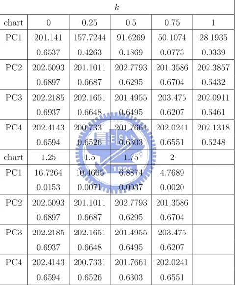
of Σ. And Figures 25-28 illustrate respectively the corresponding features captured by the first four principal components, by showing in each plot the mean profile and the profiles corresponding to the largest score and smallest score of the principal component. Now for each shift in I, M, N , we generate 200,000 profiles to computed an ARL estimate. Then repeat this 1000 times to get a more accurate estimate along with its standard error as before. Ta-bles 4-6 display the ARL values for the shifts in I, M, N , respectively. We can see from Table 4 that PC3 and PC1 can capture the shift in I. PC3 has the best power for detecting I-shift. PC2 and PC4 hardly have any power on detecting I-shift. Also, we can see from Table 5 that PC2 and PC1

out-perform the other two with PC2 slightly better than PC1 in capturing the shift in M . And for detecting N-shift, we can see from Table 6 that PC2 and PC1 are the best two. But as the shift tends to 3 units of σN, PC2 still

has the best power and PC3 becomes the second best for detecting N-shift.

In fact, we can obtain the exact ARL values as follows. Let P = (P1, P2,

· · · , P4)0, where Pi is the i-th eigenvector of Σ. Then P projects profiles

to the first four principal components. Let λ1, · · · , λ4 be the corresponding

eigenvalues of Σ. Since the in-control profile Y ∼ MV N (µ, Σ) and P ΣP0 ₌

diag(λ1, · · · , λ4) ≡ Λ4, we have the score vector P Y ∼ MV N(P µ, Λ4).

Denote the shifted profile by ˜Y and the shifted mean profile by ˜µ. Then P ˜Y ∼ MV N(P ˜µ, Λ4). Let δ = ˜µ − µ. The probability of detecting the shift

of the i-th principal component chart is

p = P (|P 0 i(Y − µ)_√ λi | ≤ Z0.0025) = P (−P_√ 0iδ λi − Z0.0025 ≤ P0 i(Y − ˜_√ µ) λi ≤ −P_√ 0iδ λi + Z0.0025) = P (−P_√ 0iδ λi − Z0.0025 ≤ Z ≤ −P0 iδ √ λi + Z0.0025),

where Z is the standard normal variate. The value 1/p is the actual ARL of the i-th principal-component chart. Tables 7-9 show respectively the actual ARL for each of the I, M, N shifts. By comparing Tables 4-9, we can see that our simulated ARLs are all very close to the actual ARLs, which verifies the correctness of the simulation.

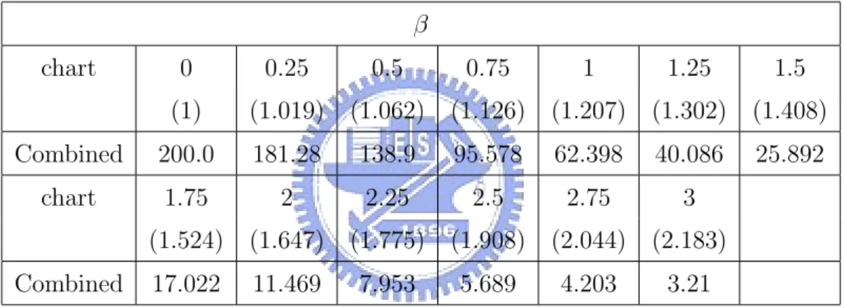
Since each of the I, M, N shifts is captured by more than one principal-component chart, we recommend using the combined chart to monitor these shifts. A combined chart means we monitor the process by more than one chart and the combined chart signals out of control if any of the charts

signals. Set the overall false-alarm rate at α = 0.005. Since these scores are independent, the individual false-alarm rate is α0 _{= 1 − (0.995)}1/4 _{for each of}

the four principal component scores. Then we can have the control limits of these four scores as shown below:

(P0 1µ − Z1−(0.995)1/4 2 p λ1, P01µ + Z1−(0.995)1/4 2 p λ1) (P0₂µ − Z1−(0.995)1/4 2 p λ2, P02µ + Z1−(0.995)1/4 2 p λ2) (P0 3µ − Z1−(0.995)1/4 2 p λ3, P03µ + Z1−(0.995)1/4 2 p λ3) (P0₄µ − Z1−(0.995)1/4 2 p λ4, P04µ + Z1−(0.995)1/4 2 p λ4)

If one of the principal component scores is out of the control limits, then this profile is claimed as out of control. That is, only when all four principal component scores of that profile are within the control limits simultaneously, then it will be treated as an in-control profile. In order to do the comparison the above, we also simulate 200,000 profiles each time to get an ARL estimate. Then repeat 1000 times to get the final ARL estimate and its standard error. Tables 10-12 display the simulation results for ARL comparison for I, M, N shifts, respectively. Also, we can derive the exact control limits and compute the exact ARL. Tables 13-15 show the ARL computed from the exact control limits with shifts in I, M, N , respectively. By comparing the simulated ARL with the exact ARL for our combined chart, we can see that they are very closed to each other. Also, we plot the ARL comparison plots for PC1, PC2, PC3, PC4 and the combined chart with I, M, N shifts in Figures 29-31 respectively. As we can see for I-shifts, PC3 dominates primarily. And for the combined chart scheme, it was the second best in monitoring the shifts in I. As the shifts gets bigger, the difference in ARL between PC3 and the combined chart gets smaller. Also, for M-shifts, PC2 is the best scheme to monitor it. For the second best one, the PC1 and the combined chart are comparable. Note that two ARL curves intersect at about 1.25σM shift. That

chart scheme outperforms PC1 as the shift size tends larger than 1.25σM.

We can see the same phenomenon in N. From Figure 31, PC2 is still the best one to monitor shifts in N. PC1 and the combined chart scheme are comparable. Also the two ARL curves intersect at about 1.1σN shift.

Also, we show the ARL values for simultaneous shifts of I and M, I and

N, and M and N, in Tables 16-18, respectively. We can see from Table 16

that PC1 takes the major job of monitoring simultaneous shifts in I and M while PC3 serves as the second best. And from Table 17, we can observe that PC2 dominates the simultaneous shifts in I and N while PC1 serves as the second best. Also from Table 18, we can see that PC1 plays the major role in monitoring simultaneous shifts in M and N while PC2 performs the second best. But notice that the power for PC2 here is not comparable with PC1.

Finally, we consider shifts in the variance of I, M, and N. Recall that the in-control situation is: I ∼ N(1, 0.22_{), M ∼ N(15, 1), N ∼ N(−1.5, 0.3}2_).

Now for variance shifts in I, we consider σI = 0.3, 0.4, . . . , 1. For each shift,

we simulate 200,000 profiles to get an ARL estimate and then repeat the procedure for 1000 times to get the mean and the corresponding standard deviation. The ARL results for each principal component chart and the com-bined chart are shown in Table 19. And Figure 32 shows the corresponding ARL curves. As we can see that PC3 dominates for the shifts in variance of I while the combined chart scheme also performs very well in monitoring this kind of shifts.

And for variance shifts in M, we consider σM = 1.5, 2, . . . , 5. The

simula-tion results are shown in Table 20 and Figure 33. Likewise, we can see that PC2 dominates for the shifts in variance of M. But here, the combined chart scheme is comparable with the PC2. As σM gets bigger, the combined chart

we consider σN = 0.4, 0.5, . . . , 1.1. Table 21 and Figure 34 shows the

simula-tion results. From these simulasimula-tion results, we can see that PC3 has the best detecting power for variance shifts in N. The combined chart scheme also has great detecting power for monitoring shifts in σN. Notice that as σN tends

bigger than 0.7, the profile shape will be greatly affected. Therefore we can see that all these four principal components are sensitive to it and they all have great detecting power. While it is difficult to figure out which principal component dominates the shifts, we recommend the combined chart scheme for monitoring.

Since the model under study is a random effect model, we are curious of the power in monitoring variance shifts. From the above simulations, we have shown that the combined chart scheme is a very good choice for monitoring random effect model. So here, in order to compare the power of our combined chart in detecting mean shifts and variance shifts, we use the ARL of the combined chart scheme. Then, use our comparison basis vef to quantify the difference between the shifted profiles and the reference profile. Hence we can have the plot that compares the ARL of detecting mean shifts and variance shifts; see Figure 35.

We can see from Figure 35 that for both I, M, N shifts, our monitoring scheme performs better in detecting variance shifts than mean shifts. We can observe that there exist big differences for all I, M, N shifts at small values of comparison basis. And as the value of comparison basis tends bigger, the difference between mean shifts and variance shifts tends smaller. When the value of comparison basis getting large enough, there exist almost no differences between mean shifts and variance shifts. Also from Figure 35, we can see that our monitoring scheme does the best job in detecting variance shifts in N while the second best one is variance shifts in I.

5

A Case Study - VDP Example

5.1

Phase I monitoring

The VDP data set contains n = 24 profiles, each was measured at p = 314 set points. Figure 2 is the plot of the VDP data. We fit these 24 profiles by B-splines with 16 degrees of freedom. See Figure 36 for the plot of the fitted B-splines. Also Figures 37-40 respectively plot principal components 1 to 4 showing the modes of variation they capture. And the first four principal components account for 0.8535, 0.1084, 0.0190, 0.0084 of variation in the profiles, respectively. The total is 0.9893. Figure 41 is the plot of the corresponding eigenvectors. Now for Phase I monitoring, we use the same method as for the aspartame example. Figures 42 and 43 are the control charts of T2

1 and T22 respectively. We can see that there are no out-of-control

profiles in the VDP data.

5.2

Phase II monitoring

Since, in the aspartame example, the first four principal components cannot distinguish the shifts in I, M, N very clearly, we suggest using the combined chart scheme to monitor these shifts. Now, we are going to demonstrate an example that its principal components can capture the shapes of shifts very clearly by simulation.

For demonstrating Phase I monitoring, we need to generate new VDP data. Applying PCA to the original VDP data, we then have the corre-sponding eigenvectors {ρ₁, · · · , ρ₃₁₄} and eigenvalues {λ1, · · · , λ314}. Since

the first four principal components can explain 97.57 percent of variation, we only use these four principal components to regenerate the new VDP data. And these first four principal components account for 0.8402, 0.1072, 0.0192, 0.0091 of variation in these profiles, respectively.

We use the following steps to regenerate a set of new VDP data.

1. Generate i.i.d. ²j,q from the normal distribution with zero mean and

variance λq, 1 ≤ j ≤ 24, 1 ≤ q ≤ 4.

2. Generate ˜Xj,k = µ(tk) +

P₄

q=1²j,q· ρq(tk), 1 ≤ j ≤ 24, 1 ≤ k ≤ 314.

Note that λ1, λ2, λ3, λ4 are the four largest eigenvalues and ρ1, ρ2, ρ3, ρ4

are the corresponding eigenvectors with length 314. And µ(·) is the mean profile of the 24 original VDP curves where tk denotes the k-th set point.

Figure 44 displays the simulated VDP data. We can see that the simulated data do capture the peaks and the shapes of the original VDP data.

Then, we apply our estimation method to the generated data to get the simulated mean profile, eigenvalues, and eigenvectors. Figure 45 displays the mean profile of the real data and the simulated data. We can see that these two curves are very close. Figures 46-49 show the first four eigenvectors of the real data and that of the simulated data, respectively. Likewise, from these four figures we can see that the simulated eigenvectors are all close to that of the real data. Also, Figure 50 shows that the simulated eigenvalues are fairly close to the eigenvalues of the original profile data. Therefore, we can say that the data generation method we adopt here can really capture the shapes and variations of the original data.

In Phase II monitoring, we treat the average profile vector µ of the 24 smoothed VDP profiles and the sample covariance matrix Σ as the in-control process parameters to perform our simulation. Here, µ = (µ(t1), · · · , µ(t314))0

is a 314 × 1 vector and the covariance matrix Σ is a 314×314 matrix. We can generate the in-control profiles by Y ∼ MV N (µ, Σ). For out-of-control conditions, we shift the profiles in their first two principal components. That is, generate new profile data by

˜

where k=0, 0.25, . . . , 2 and vi is the i-th eigenvector of Σ, i=1, 2. We

sim-ulated 200,000 profiles to compute an ARL estimate for each out-of-control conditions considered. Then we repeat the procedure 1000 times to get our final ARL estimate along with its standard error. Tables 22 and 23 report the ARL results for shifts in principal component 1 and principal component 2 respectively.

As we can see from Table 22 that shifts in principal component 1 are solely captured by the first principal component score. Likewise, from Ta-ble 23, shifts in principal component 2 are captured by the second principal component score. The other three principal component scores make no con-tributions to the power of detection.

6

Conclusions

The monitoring of process or product profiles is a very popular and promising area of research in statistical process control in recent years. In this study, we discuss monitoring schemes for the random effect nonliner profiles. We use the principal component analysis to analyze the covariance matrix of the profile data and use the corresponding principal component scores that capture the main features of these profile data for process monitoring.

In the study of the aspartame example, our simulation shows that prin-cipal component 3 performs the best over the entire range of I shifts. And principal component 2 is the best for monitoring M shifts while principal component 1 also plays an important role in monitoring M shifts. And for shifts in N, principal component 2 performs the best over the entire range. Likewise, principal component 1 also plays an important role in monitoring

N shifts. Note that as the shift tends bigger in N shift, all those four

each shift, we can also use the combined chart to perform monitoring. We have shown that although this monitoring scheme may not be the best for each shift, it still has comparably good power to monitor these shifts. More-over, we have displayed in the tables the results when two of I, M, N shift simultaneously.

Using the example of vertical density profiles, we demonstrate that when the shift corresponds to a mode of variation that a particular principal ponent represents, then we can directly use the score of that principal com-ponent to perform monitoring.

So if a principal component can clearly identify the shift, a situation may be rare in real applications, then we recommend monitoring the score of that principal component. Otherwise we recommend the combined chart scheme because it still has comparably good power to monitor these shifts.

Moreover, we use a mean-squares-error-like (MSE-like) measure as a com-parison basis to compare the ARL performance in mean shifts and variance shifts. Simulation results indicate that our monitoring scheme performs bet-ter in detecting variance shifts. And in the selection of number of principal components, we adopt the cross-validation method for its popularity and simplicity. Also, in the use of cross-validation, we have observed that the se-lection is affected by the number of groups that the data set is divided into. By our simulation result, we can see that as the number of groups increases, the selected number of principal components decreases. Further studies are needed on this issue.

Finally in the studies of Phase I monitoring, we compare T2

1 and T22. And

we show by simulation that T2

1 has a better overall performance than T22

References

[1] Anderson, T. W. (2003). An Introduction to Multivariate Statistical

Analysis, 3rd edition. Wiley, New York.

[2] Castro, P. E., Lawton, W. H., and Sylvestre, E. A. (1986). “Principal Modes of Variation for Processes With Continuous Sample Curves”. Technometrics 28, pp. 329–337.

[3] de Boor, C. (1978). A Practical Guide to Splines. Springer, Berlin. [4] Jackson, J. E. (1991). A User’s Guide to Principal Components.

Wi-ley, New York.

[5] Jones, M. C. and Rice, J. A. (1992). “Displaying the Important Fea-tures of Large Collections of Similar Curves”. The American Statistician, Vol. 46, No. 2, pp. 140–145.

[6] Kang, L. and Albin, S. L. (2000). “On-Line Monitoring When the Process Yields a Linear Profile”. Journal of Quality Technology 32, pp. 418–426.

[7] Kim, K., Mahmoud, M. A., and Woodall, W. H. (2003). “On the Monitoring of Linear Profiles ”. Journal of Quality Technology 35, pp. 317–328.

[8] Ramsay, J. O. and Silverman, B. W. (2002). Applied Functional

Data Analysis: Methods and Case Studies. Springer, New York.

[9] Rice, J. A. and Silverman, B. W. (1991). “Estimating the Mean and Covariance Structure Nonparametrically When the Data Are Curves”.