混合偏斜t分佈及其應用

國 立 交 通 大 學

統計學研究所

碩 士 論 文

混合偏斜t分佈及其應用

On the mixture of skew t distributons

and its applications

研 究 生 ：謝宛茹

指導教授 ：李昭勝 博士

林宗儀 博士

混合偏斜t分佈及其應用

On the mixture of skew t distributions

and its applications

研 究 生：謝宛茹

Student ： Wan-Ju Hsieh

指導教授：李昭勝

Advisors： Dr. Jack C. Lee

林宗儀

Dr. Tsung I. Lin

國 立 交 通 大 學

統計學研究所

碩 士 論 文

A Thesis

Submitted to Institute of Statistics

College of Science

National Chiao Tung University

in Partial Fulfillment of the Requirements

for the Degree of

Master

in

Statistics

June 2006

Hsinchu, Taiwan, Republic of China

中華民國九十五年六月

混合偏斜t分佈及其應用

研究生：謝宛茹 指導教授：李昭勝 博士

林宗儀 博士

國立交通大學統計學研究所

摘要

混合 t 分佈已被認為是混合常態分佈的一種具穩健性的延伸。近年

來, 處理具異質性並牽涉了具不對稱現象的資料問題中, 混合偏斜常態

分佈已經被驗證是一種很有效的工具。本文我們提出一種具穩健性的混

合偏斜 t 分佈模型來有效地處理當資料同時具有厚尾、偏斜與多峰型式

的現象。除此之外, 混合常態分佈(NORMIX)、混合 t 分佈(TMIX)與混

合偏斜常態分佈(SNMIX)模型皆可視為本篇論文所提出混合偏斜 t 分佈

(STMIX)的特例。我們建立一些 EM-types 演算法, 以遞迴的方式去求最

大概似估計值。最後, 我們也透過分析一組實例來闡述我們所提出來方

法。

On the mixture of skew t distributions

and its applications

Student：Wan-Ju Hsieh Advisors：Dr. Jack C. Lee

Dr. Tsung I. Lin

Institute of Statistic

National Chiao Tung University

ABSTRACT

A finite mixture model using the Student's t distribution has been

recognized as a robust extension of normal mixtures. Recently, a mixture of

skew normal distributions has been found to be effective in the treatment of

heterogeneous data involving asymmetric behaviors across subclasses. In

this article, we propose a robust mixture framework based on the skew t

distribution to efficiently deal with heavy-tailedness, extra skewness and

multimodality in a wide range of settings. Statistical mixture modeling based

on normal, Student's t and skew normal distributions can be viewed as

special cases of the skew t mixture model. We present some analytically

simple EM-type algorithms for iteratively computing maximum likelihood

estimates. The proposed methodology is illustrated by analyzing a real data

example.

誌謝

研究所兩年的生涯，這快樂、充實、努力的日子匆匆過去了。此時此刻，即將 要畢業的我，回想著過去兩年的研究生活、生活點滴，期待與不捨的情緒百感交集。 我的心情是充滿了感激與感動。 論文得以順利完成，首先要感謝的就是我的指導教授李昭勝老師，老師豐富的 學識涵養對於學生的關心和照顧，讓我如沐春風、心存感激，身為李老師的學生讓 我覺得很驕傲也很開心；另一位對於這篇論文貢獻最大的是林宗儀學長，經由學長 的用心指導，才能順利的完成，在這裡要感謝學長不辭辛勞的指導；另外還要感謝 所上老師們的用心授課，使我受益良多；接著還要感謝口試委員趙蓮菊老師和彭南 夫老師，特地抽空參加並給予我寶貴的意見。謝謝你們。 接著要感謝我的好朋友，包括了婉文、沛君、孟樺、大宛、鷰筑、秀慧和小馬， 因為有你們這一群朋友陪伴，為我的研究生生涯帶來了歡笑與淚水，因為有你們的 扶持與鼓勵，使得這些日子充滿了溫馨與感動。另外要特別感謝我的室友婉文和沛 君，總是在我面臨低潮時，為我加油、打氣，互相鼓舞著對方給彼此動力，讓我在 寫論文的這段期間，產生了有福同享、有難同當的患難真情，我會永遠珍惜的。接 著還要感謝我最重要的朋友－泰彬，從大學以來，謝謝你一路走來對我的包容與照 顧，你總是默默的支持我，給我最大的信心與鼓勵，適時的給予我溫暖與幫助，因 為有你，讓我一路有所依靠，使我對自己有更的信心與動力，更有勇氣面對挫折與 挑戰。 最後我要感謝我的家人－父親謝日春、母親鄭秀鳳、弟弟國鼎和妹妹蓓雅，感 謝他們給我一個溫馨又快樂的家庭，總是在背後默默的支持我，鼓勵我，讓我無後 顧之憂的為自己的理想努力，得以順利完成論文。在鳳凰花開、驪歌輕唱之際，謹 以本文獻給所有的至親與好友，與你們分享我的喜悅。 謝宛茹 謹誌于 國立交通大學統計學研究所 中華民國九十五年六月十日

Contents

1. INTRODUCTION 2

2. PRELIMINARIES 4

3. ML ESTIMATION OF THE SKEW t DISTRIBUTION 9 4. THE SKEW t MIXTURE MODEL 13

5. AN ILLUSTRATIVE EXAMPLE 19

6. CONCLUDING REMARKS 23

List of Tables

1 ML estimation results for fitting various mixture models on the BMI adult men example. . . 21

List of Figures

1 Plots of standard skew normal densities (dashed lines) and standard skew t densities (solid lines) with ν = 5 under various λ. . . . 6

2 The skewness and kurtosis plots versus λ for the standard skew t distribution with ν = 5. . . . 6

3 Plot of the profile log-likelihood of the degrees of freedom ν for fitting the bmimen data with a two component STMIX model with equal degrees of freedom (ν1 = ν2 = ν). . . . 20

4 Histogram of the bmimen data with overlaid four ML-fitted two com-ponent mixture densities (normal, Student’s t, skew normal and skew

t). . . . 22

5 Empirical cdf of the bmimen data together with two superimposed cdfs from the ML-fitted two component SNMIX and STMIX models. 22

On the mixture of skew t distributons

and its applications

Student: Wan-Ju Hsieh

Advisors:

Dr. Jack C. Lee

Dr. Tsung I. Lin

Institute of Statistics National Chiao Tung University

Hsinchu, Taiwan

Abstract

A finite mixture model using the Student’s t distribution has been recog-nized as a robust extension of normal mixtures. Recently, a mixture of skew normal distributions has been found to be effective in the treatment of hetero-geneous data involving asymmetric behaviors across subclasses. In this article, we propose a robust mixture framework based on the skew t distribution to efficiently deal with heavy-tailedness, extra skewness and multimodality in a wide range of settings. Statistical mixture modeling based on normal, Stu-dent’s t and skew normal distributions can be viewed as special cases of the skew t mixture model. We present some analytically simple EM-type algo-rithms for iteratively computing maximum likelihood estimates. The proposed methodology is illustrated by analyzing a real data example.

Key words: EM-type algorithms; Heterogeneity data; Maximum likelihood;

1.

INTRODUCTION

The normal mixture (NORMIX) model has been found to be one the most popular model-based approaches to dealing with data in the presence of population

heterogeneity in the sense that data intrinsically consist of unlabelled observations,

each of which is thought to belong to one of g classes (or components). For a com-prehensive list of applications and an abundant literature survey on this area, see Titterington, Smith and Markov (1985), McLachlan and Basford (1988), McLachlan and Peel (2000), and Fraley and Raftery (2002). It is well known that the t distribu-tion involves an addidistribu-tional turning parameter (the degrees of freedom) that is useful for outlier accommodation. Over the past few years, there has been considerable attention to a robust mixture context based on the Student’s t distribution, which we call the t mixture (TMIX) model. Recent developments about TMIX models in-clude Peel and McLachlan (2000), Shoham (2002), Shoham, Fellows, and Normann (2003), Lin, Lee, and Ni (2004) and Wang et al. (2004), among others.

While NORMIX and TMIX models have been well recognized as useful in many practical applications, data with varying degrees of extreme skewness among sub-classes may not be well modeled. In attempting to appropriately model a set of data arising from a class or several classes with asymmetric observations, Lin, Lee and Yen (2006) recently introduced a new mixture model with each unseen component following a skew normal distribution (Azzalini 1985, 1986). A skew normal mixture (SNMIX) model for a continuous random variable Y is of the form

Y ∼ g X i=1 wif (y|ξi, σi2, λi), ωi ≥ 0, g X i=1 ωi = 1, (1)

where g is the number of components, wi’s are mixing probabilities and f (y|ξi, σi2, λi) = 2 √ 2πσi exp µ −(y − ξi)2 2σ2 i ¶ Z _λi(y−ξi) σi −∞ 1 √ 2πexp µ −x2 2 ¶ dx

is a skew normal density function with location parameter ξi ∈ R, scale parameter

σ2

i > 0 and skewness parameter λi ∈ R. As described in Lin, Lee and Yen (2006),

the SNMIX model (1) can be represented by a normal-truncated normal-multinomial hierarchial structure. Such representation leads to a convenient implementation for maximum likelihood (ML) estimation under a complete-data framework.

Although model (1) offers great flexibility in modeling data with varying asym-metric behaviors, it may suffer from a lack of robustness regarding extreme outlying observations. In general, the skewness parameters could be unduly affected by observations that are atypical within components in model (1) being fitted. This motivates us to develop a wider class of mixture distributions to accommodate asym-metry and long tails simultaneously. In this paper, we are devoted to the fitting of mixture of skew t distributions, introduced by Azzalini and Capitaino (2003), allowing heavy tails in addition to skewness as a natural extension of Lin, Lee and Yen (2006). With this skew t mixture (STMIX) model approach, the NORMIX, TMIX and SNMIX models can be treated as special cases in this family.

The rest of the paper is organized as follows. Section 2 briefly outlines some preliminary properties of the skew t distribution. Section 3 presents the imple-mentation of ML estimation for fitting the skew t distribution via three simple extensions/modifications of the EM algorithm (Dempster, Laird and Rubin 1977), including the ECM algorithm (Meng and Rubin 1993), the ECME algorithm (Liu and Rubin 1994), and the PX-EM algorithm (Liu, Rubin and Wu 1998). Section 4 discusses the STMIX model and presents the implementation of EM-type algo-rithms for obtaining ML estimates of the parameters. Moreover, we offer a simple

way to calculate the information-based standard errors instead of using computation-ally intensive resampling techniques. In Section 5, the application of the proposed methodology is illustrated through real data of body mass indices measuring from the U.S. male adults. Some concluding remarks are given in Section 6.

2.

PRELIMINARIES

For computational ease and notational simplicity, throughout this paper we de-note by φ(·) and Φ(·) respectively the probability density function (pdf) and the cumulative distribution function (cdf) of the standard normal distribution and de-note by tν(·) and Tν(·) respectively the pdf and the cdf of the Student’s t distribution

with degrees of freedom ν. We start by defining the skew t distribution and its hi-erarchical formulation and then introduce some further properties.

A random variable Y is said to follow the skew t distribution ST (ξ, σ2_{, λ, ν) with}

location parameter ξ ∈ R, scale parameter σ2 _{∈ (0, ∞), skewness parameter λ ∈ R}

and degrees of freedom ν ∈ (0, ∞) if it has the following representation:

Y = ξ + σ√Z

τ, Z ∼ SN (λ), τ ∼ Γ(ν/2, ν/2), Z ⊥ τ, (2)

where SN (λ) stands for the standard skew normal distribution, has a pdf given by

f (z) = 2φ(z)Φ(λz), z ∈ R, Γ(α, β) is the gamma distribution with mean α/β, and

the symbol ‘⊥’ indicates independence.

The following result, as provided by Azzalini and Capitanio (2003), is useful for evaluating some integrals that we use in the rest of the paper:

Proposition 1. If τ ∼ Γ(α, β), then for any a ∈ R

E ³ Φ(a√τ ) ´ = T2α µ a r α β ¶ .

By Proposition 1, integrating τ from the joint density of (Y, τ ) will lead to the following marginal density of Y :

f (y) = 2 σtν(η)Tν+1 µ λη r ν + 1 η2_{+ ν} ¶ , η = y − ξ σ . (3)

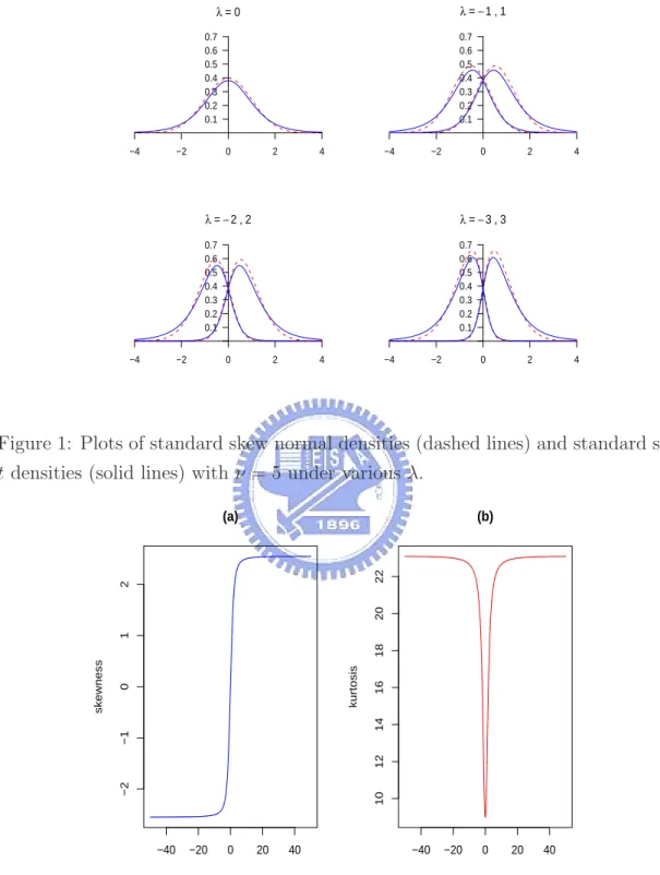
Note that as ν → ∞, τ → 1 with probability 1 and Y = ξ + σZ. Figure 1 shows the plots of standard skew normal distributions superimposed the standard skew t distributions with ν = 5 under λ = 0, ±1, ±2, ±3.

Standard algebraic manipulations yield the following:

E(Y ) = ξ +Γ((ν − 1)/2) Γ(ν/2) r ν πδλσ. (4) var(Y ) = σ2_ν ½ 1 2 Γ((ν − 2)/2) Γ(ν/2) − δ2 λ π ³Γ((ν − 1)/2) Γ(ν/2) ´₂¾ . (5) γY = 1 2 ½ πδλ ¡ 3 − δ2 λ)Γ µ ν − 3 2 ¶ Γ³ν 2 ´₂ −3πδλΓ µ ν − 2 2 ¶ Γ µ ν − 1 2 ¶ Γ³ν 2 ´ + 4δ3 λΓ µ ν − 1 2 ¶₃¾ × ½ π 2Γ µ ν − 2 2 ¶ Γ³ν 2 ´ − δ2 λΓ µ ν − 1 2 ¶₂¾_−3/2 . (6) κY = ½ 3π2_Γ µ ν − 4 2 ¶ Γ³ν 2 ´₃ − 8πδ2 λ(3 − δ2)Γ µ ν − 3 2 ¶ Γ µ ν − 1 2 ¶ Γ³ν 2 ´₂ +12πδ2 λΓ µ ν − 2 2 ¶ Γ µ ν − 1 2 ¶₂ Γ³ν 2 ´ − 12δ4 λΓ µ ν − 1 2 ¶₄¾ × ½ πΓ µ ν − 2 2 ¶ Γ³ν 2 ´ − 2δ2 λΓ µ ν − 1 2 ¶₂¾₋₂ . (7) where δλ = λ/ √ 1 + λ2_{, and γ}

Y and κY are the measures of skewness and kurtosis,

respectively. Figure 2 displays the γY and κY as a function of λ for the standard

skew t distribution with ν = 5. The sketch of the proofs of Eqs (4)-(7) are given in Appendix A.

−4 −2 0 2 4 0.1 0.2 0.3 0.4 0.5 0.6 0.7 λ =0 −4 −2 0 2 4 0.1 0.2 0.3 0.4 0.5 0.6 0.7 λ = −1,1 −4 −2 0 2 4 0.1 0.2 0.3 0.4 0.5 0.6 0.7 λ = −2,2 −4 −2 0 2 4 0.1 0.2 0.3 0.4 0.5 0.6 0.7 λ = −3,3

Figure 1: Plots of standard skew normal densities (dashed lines) and standard skew

t densities (solid lines) with ν = 5 under various λ.

−40 −20 0 20 40 −2 −1 0 1 2 λ skewness (a) −40 −20 0 20 40 10 12 14 16 18 20 22 λ kurtosis (b)

Figure 2: The skewness and kurtosis plots versus λ for the standard skew t distrib-ution with ν = 5.

As shown by Azzalini (1986, p. 201) and Henze (1986, Theorem 1), a stochastic representation of Z ∼ SN (λ) is Z = δλ|U1| + p 1 − δ2 λU2, where δλ = λ/ √ 1 + λ2_,

and U1 and U2 are independent N(0, 1) random variables. This yields a further

hierarchical representation of (2) in the following:

Y | γ, τ ∼ N µ ξ + δλγ, 1 − δ2 λ τ σ 2 ¶ , γ | τ ∼ T N µ 0,σ2 τ ; [0, ∞) ¶ , τ ∼ Γ(ν/2, ν/2), (8)

where T N (µ, σ2_{; C) represents the truncated normal distribution with N (µ, σ}2₎

lying within a truncated interval C ⊂ R. From (8), the joint pdf of Y, γ, τ is given by

f (γ, τ, y) = 1 πp1 − δ2 λσ2 (ν/2)ν2 Γ(ν/2)τ ν 2 exp ³ − τ 2(1 − δ2 λ) η2 ´ exp ³ − τ 2ν ´ × exp µ − γ2τ 2(1 − δ2 λ)σ2 + γτ (1 − δ2 λ)σ2 δλ(y − ξ) ¶ . (9)

Integrating out γ in (9), we get

f (τ, y) = r 2 π 1 στ ν−1 2 (ν/2) ν 2 Γ(ν/2)exp ³ − τ 2(η 2_{+ ν)}´_Φ³_λη√_τ´_{. (10)} Dividing (9) by (10) gives f (γ | τ, y) = √1 2π √ τ σp1 − δ2 λ exp ³ − τ ¡ γ − (y − ξ)δλ ¢₂ 2(1 − δ2_)σ2 ´ Φ−1³_λη√_τ´_{. (11)}

It follows from (11) that the conditional distribution of γ given τ and Y is

γ | τ, Y ∼ T N µ δλ(y − ξ), (1 − δ2 λ)σ2 τ ; (0, ∞) ¶ . (12)

From (10), applying Proposition 1 yields the conditional density of τ given Y

f (τ | y) = bτ(ν−1)/2exp ³ − τ 2 ¡ η2+ ν¢´Φ ³ λη√τ ´ , (13) where b = µ η2_{+ ν} 2 ¶(ν+1)/2½ Γ µ ν + 1 2 ¶ Tν+1 µ λη r ν + 1 η2_{+ ν} ¶¾−1 (14) is the normalizing constant.

Proposition 2. Given the hierarchical representation (8), we have the following:

(a) The conditional expectation of τ given Y = y is E(τ |y) = µ ν + 1 η2 _{+ ν} ¶ Tν+3 ³ Mqν+3 ν+1 ´ Tν+1(M) , where M = ληqν+1 η2_+ν.

(b) The conditional expectation of γτ given Y = y is E(γτ |y) = δλ(y − ξ)E(τ |y) +

p 1 − δ2 λ πfY(y) µ η2 ν(1 − δ2 λ) + 1 ¶_−(ν/2+1) .

(c) The conditional expectation of γ2_{τ given Y = y is} E(γ2τ |y) = δ_λ2(y − ξ)2E(τ |y) + (1 − δ_λ2)σ2

+δλ(y − ξ) p 1 − δ2 λ πfY(y) µ η2 ν(1 − δ2 λ) + 1 ¶_−(ν/2+1) .

(d) The conditional expectation of log(τ ) given Y = y is E¡log(τ )|y¢ = DG µ ν + 1 2 ¶ − log³η2+ ν 2 ´ + ν + 1 η2_{+ ν}  Tν+3 ³ M q ν+3 ν+1 ´ Tν+1(M) − 1   + λη(η 2 _{− 1)} p (ν + 1)(ν + η2₎3 tν+1(M) Tν+1(M) + 1 Tν+1(M) Z _M −∞ gν(x)tν+1(x)dx, and gν(x) = DG µ ν + 2 2 ¶ − DG µ ν + 1 2 ¶ − log µ 1 + x 2 ν + 1 ¶ + (ν + 1)x 2_{− ν − 1} (ν + 1)(ν + 1 + x2₎, (15) where DG(x) = Γ0_{(x)/Γ(x) is the digamma function.}

3.

ML ESTIMATION OF THE SKEW t DISTRIBUTION

In this section, we demonstrate how to employ the EM-type algorithms for ML estimation of the skew t distribution, which can be viewed as a single component skew t mixture model that we shall discuss in the next section. From the represen-tation (8), n independent observations from ST (ξ, σ2_{, λ, τ ) can be expressed by}

Yj | γj, τj ind∼ N µ ξ + δλγj, 1 − δ2 λ τj σ2 ¶ , γj | τi ind∼ T N µ 0,σ 2 τj ; (0, ∞) ¶ , τj ind∼ Γ(ν/2, ν/2) (j = 1, . . . , n).

Letting y = (y1, . . . , yn), γ = (γ1, . . . , γn) and τ = (τ1, . . . , τn), the complete

data log-likelihood function of θ = (ξ, σ2_{, λ, ν) given (y, γ, τ ), ignoring additive}

constant terms, is given by

`c(θ | y, γ, τ ) = −ν 2 n X i=1 τj− n X j=1 ³ _η2 jτj 2(1 − δ2 λ) ´ + n X j=1 µ δληjγjτj (1 − δ2 λ)σ ¶ − n X j=1 ³ _γ j2τj 2(1 − δ2 λ)σ2 ´ −n log σ2− n 2 log(1 − δ 2 λ) + nν 2 log ³ν 2 ´ − n log Γ³ν 2 ´ +ν 2 n X j=1 log τj, where ηj = (yj− ξ)/σ.

By Proposition 2, given the current estimate ˆθ(k) = (ˆξ(k)_{, ˆσ}2(k)

, ˆλ(k)_{, ˆν}(k)_{) at the} kth iteration, the expected complete data log-likelihood function (or the Q-function

as asserted in Dempster Laird, and Rubin 1977) is

Q(θ | ˆθ(k)) = −ν 2 n X j=1 ˆ s(k)_1j − n X j=1 ³ η2 jsˆ(k)1j 2(1 − δ2 λ) ´ + n X j=1 µ δληjsˆ(k)2j (1 − δ2 λ)σ ¶ − n X j=1 ³ _sˆ(k) 3j 2(1 − δ2 λ)σ2 ´ −n log σ2₋ n 2log(1 − δ 2 λ) + nν 2 log ³ν 2 ´ − n log Γ³ν 2 ´ +ν 2 n X j=1 ˆ s(k)_4j , (16)

where ˆ s(k)_1j = E(τj|yj, ˆθ (k) ) = à ˆ ν(k)_{+ 1} ˆ η2(k) j + ˆν(k) ! T_νˆ(k)₊₃ ³ ˆ M_j(k) q ˆ ν(k)₊₃ ˆ ν(k)₊₁ ´ T_νˆ(k)₊₁ ³ ˆ M_j(k) ´ , (17) ˆ s(k)_2j = E(γjτj|yj, ˆθ (k) ) = ˆδ_λ(k)(yj− ˆξ(k))ˆs(k)1j + q 1 − ˆδ2(k) λ π ˆf_Y(k)_j (yj) µ ˆ η2(k) j ˆ ν(k)_{(1 − δ}2(k) λ ) + 1 ¶_−(ˆν(k)_/2+1) , (18) ˆ s(k)_3j = E(γ_j2τj|yj, ˆθ (k) ) = ˆδ2(k) λ (yj− ˆξ(k))2sˆ(k)1j + (1 − ˆδ2 (k) λ )ˆσ2 (k) + ˆ δ(k)_λ (yj − ˆξ(k)) q 1 − ˆδ2(k) λ π ˆf_Y(k)_j (yj) µ ˆ η2(k) j ˆ ν(k)_{(1 − ˆδ}2(k) λ ) + 1 ¶_−(ˆν(k)_/2+1) , (19) and ˆ s(k)_4j = E(log τj|yj, ˆθ (k) ) = DG µ ˆ ν(k)_{+ 1} 2 ¶ + νˆ(k)+ 1 ˆ η2(k) j + ˆν(k)    T_ˆν(k)₊₃ ³ ˆ M_j(k) q ˆ ν(k)₊₃ ˆ ν(k)₊₁ ´ T_νˆ(k)₊₁ ¡ _ˆ M_j(k)¢ − 1    − log³ ˆη 2(k) j + ˆν(k) 2 ´ + λˆ (k)_ηˆ(k) j (ˆη2 (k) j − 1) q (ˆν(k)_{+ 1)(ˆν}(k)_{+ ˆη}2(k) j )3 à t_νˆ(k)₊₁( ˆM_j(k)) T_νˆ(k)₊₁( ˆM_j(k)) ! + 1 T_ˆν(k)₊₁ ¡ _ˆ M_j(k)¢ Z _Mˆ(k) j −∞ g_νˆ(k)(x)t_νˆ(k)₊₁(x)dx, (20) with ˆ η_j(k) = yj− ˆξ (k) ˆ σ(k) , δˆ (k) λ = ˆ λ(k) p 1 + ˆλ2(k), ˆ M_j(k) = ˆλ(k)ηˆ(k)_j s ˆ ν(k)_{+ 1} ˆ η2(k) j + ˆν(k) , ˆ f_Y(k)_j (yj) = 2 ˆ σ(k)tνˆ(k)(ˆη (k) j )Tνˆ(k)₊₁ ¡ _ˆ M_j(k)¢.

Our proposed ECM algorithm for the skew t distribution consists of an EM-step and four CM-steps as described below:

E-step: Given θ = ˆθ(k), compute ˆs(k)_1j , ˆs_2j(k), ˆs(k)_3j and ˆs(k)_4j in Eqs (17)-(20) for

j = 1, . . . , n.

CM-step 1: Update ˆξ(k) _{by maximizing (16) over ξ, which leads to}

ˆ ξ(k+1) = P_n j=1sˆ (k) 1j yj− ˆδ(k)λ P_n j=1ˆs (k) 2j P_n j=1sˆ (k) 1j .

CM-step 2: Fix ξ = ˆξ(k+1)_{, update ˆσ}2(k)

by maximizing (16) over σ2_{, which gives}

ˆ σ2(k+1) = P_n j=1 ³ ˆ s(k)_1j (yj − ˆξ(k+1))2− 2ˆδ(k)λ sˆ (k) 2j (yj − ˆξ(k+1)) + ˆs(k)3j ´ 2n(1 − ˆδ2(k) λ ) .

CM-step 3: Fix ξ = ˆξ(k+1) _{and σ}2 _{= ˆσ}2(k+1)

, obtain ˆλ(k+1) _{as the solution of} nδλ(1 − δλ2) − δλ µ_Xn j=1 ˆ s(k)_1j (yj − ˆξ(k+1))2 ˆ σ2(k+1) + n X j=1 ˆ s(k)_3j ˆ σ2(k+1) ¶ +(1 + δ2 λ) n X j=1 ˆ s(k)_2j (yj − ˆξ(k+1)) ˆ σ2(k+1) = 0. CM-step 4: Fix ξ = ˆξ(k+1)_{, σ}2 _{= ˆσ}2(k+1)

and λ = ˆλ(k+1)_{, obtain ˆν}(k+1) _{as the}

solution of log³ν 2 ´ + 1 − DG³ν 2 ´ + 1 n n X j=1 ¡ ˆ s(k)_4j − ˆs(k)_1j ¢= 0.

Note that the CM-Steps 3 and 4 require a one-dimensional search for the root of

λ and ν, respectively, which can be easily achieved by using the ‘uniroot’ function

built in R. As pointed out by Liu and Rubin (1994), the one-dimensional search involved in CM-steps 3 and 4 can be very slow in some situations. To circumvent this obstacle, one may use a more efficient ECME algorithm, which refers to some conditional maximization (CM) steps of the ECM algorithm replaced by steps that maximize a restricted actual log-likelihood function, called the ‘CML-step’. With

the simple modifications, the ECME algorithm for fitting the skew t distribution can be performed by changing CM-steps 3 and 4 of the above ECM algorithm to a single CML-step as follows:

CML-step: Update λ(k) _{and ν}(k) _{by optimizing the following constrained actual}

log-likelihood function: (λ(k+1)_{, ν}(k+1)_{) = argmax} λ,ν n X j=1 log ½ tν(ηj(k+1))Tν+1 Ã λη_j(k+1) s ν + 1 η2(k+1) j + ν ! ¾ .

Another strategy for speeding up convergence rate is to use the PX-EM algorithm of Liu, Rubin and Wu (1998), which can be simply done by replacing the CM-steps 2 and 4 in the previous ECM algorithm with the following two PX.CM steps:

PX.CM-step 2: ˆ σ2(k+1) = P_n j=1 ³ ˆ s(k)_1j (yj − ˆξ(k+1))2− 2ˆδ_λ(k)sˆ(k)2j (yj − ˆξ(k+1)) + ˆs(k)3j ´ 2(1 − ˆδ2(k) λ ) P_n j=1sˆ (k) 1j . PX.CM-step 4: log à nν 2Pn_j=1sˆ(k)_1j ! − DG(ν 2) + 1 n n X j=1 ˆ s(k)_4j = 0.

Assuming that the regularity conditions in Zacks (1971, Chap. 5) hold, these guarantee that asymptotic covariance of the ML estimates can be estimated by the inverse of the observed information matrix, Io(ˆθ; y) =

P_n j=1uˆjuˆTj, where ˆ uj = ∂ log f (yj) ∂θ ¯ ¯ ¯ θ=_θˆ

Expressions for the elements of the score vector with respect to ξ, σ2_{, λ and ν} are given by ∂ log f (yj) ∂ξ = ηj σ ³ ν + 1 η2 j + ν ´ −λν σ s ν + 1 (η2 j + ν)3 tν+1(Mj) Tν+1(Mj) , ∂ log f (yj) ∂σ = ν σ ³ η2 j − 1 η2 j + ν ´ − λνηj σ s ν + 1 (η2 j + ν)3 tν+1(Mj) Tν+1(Mj) , ∂ log f (yj) ∂λ = ηj s ν + 1 η2 j + ν tν+1(Mj) Tν+1(Mj) , ∂ log f (yj) ∂ν = 1 2 ( DG(ν + 1 2 ) − DG( ν 2) − log ³ 1 + η 2 j ν ´ + η 2 j − 1 η2 j + ν + ληj ¡ η2 j − 1 ¢ q (ν + 1)¡η2 j + ν ¢_3Ttν+1_ν+1(M_(Mj_j)₎+ _Tν+11_(Mj) Z _Mj −∞ gν(x)tν+1(x)dx ) , where ηj = σ−1(yj − ξ) and Mj = ληj q ν+1 η2 j+ν.

4.

THE SKEW t MIXTURE MODEL

We consider a g-component mixture model (g > 1) in which a set of random sample Y1, . . . , Yn arises from a mixture of skew t distributions, given by

ψ(yj | Θ) = g X i=1 wif (yj | ξi, σi2, λi, νi), wi ≥ 0, g X i=1 wi = 1, (21)

where Θ = (θ1, . . . , θg) with θi = (wi, ξi, σi2, λi, νi) denoting the unknown

para-meters of component i, and wi’s being the mixing probabilities. In the mixture

context, it naturally provides a flexible framework for modeling unobserved

popula-tion heterogeneity in the collected sample. With this phenomenon, for each Yj, it

is convenient to introduce a set of zero-one indicator variables Zj = (Z1j, . . . , Zgj)T

(j = 1, . . . , n) to describe the unknown population membership. Each Zj is a

Zj ∼ M(1; w1, . . . , wg). Note that the rth element Zrj = 1 if Yj arises from the

com-ponent r. With the inclusion of indicator variables Z0

js, a hierarchical representation of (21) is given by Yj | γj, τj, zij = 1 ∼ N ³ ξi+ δλiγj, 1 − δλi 2 τj σ_i2 ´ , γj | τj, zij = 1 ∼ T N ³ 0,σ2i τj ; (0, ∞) ´ , τj | zij = 1 ∼ Γ(νi/2, νi/2), Zj ∼ M(1; w1, w2, . . . , wg). (22)

It follows from the hierarchical structure (22) on the basis of the observed data

y and latent variables γ, τ and Zj’s that the complete data log-likelihood function

of Θ, ignoring constants, is `c(Θ) = n X j=1 g X i=1 Zij ½ log wi− νiτj 2 − τjηij2 2(1 − δ2 λi) + δλiηijγjτj (1 − δ2 λi)σi − γj2τj 2(1 − δ2 λi)σ 2 i −1 2log(1 − δ 2 λi) − log σ 2 i + νi 2 log νi 2 − log ³ Γ³νi 2 ´´ +νi 2 log τj ¾ , (23) where ηij = (yj− ξi)/σi and δλi = λi/ p 1 + λ2 i. Let ˆz(k)_ij = E(Zij|yj, ˆΘ (k) ), ˆs(k)_1ij = E(Zijτj|yj, ˆΘ (k) ), ˆs(k)_2ij = E(Zijγjτj|yj, ˆΘ (k) ) ˆ s(k)_3ij = E(Zijγj2τj|yj, ˆΘ (k)

) and ˆs(k)_4ij = E(Zijlog(τj)|yj, ˆΘ

(k)

) be the necessary condi-tional expectations of (23) for obtaining the Q-function at the kth iteration. These expressions, for i = 1, . . . , g and j = 1, . . . , n, are given by

ˆ z_ij(k)= w (k) i f (yj | ξi(k), σ2 (k) i , λ (k) i , ν (k) i ) ψ(yj| ˆΘ (k) ) , (24) ˆ s(k)_1ij = ˆz(k)_ij à ˆ ν_i(k)+ 1 ˆ η2(k) ij + ˆν (k) i ! T_νˆ(k) i +3 µ ˆ M_ij(k) r ˆ νi(k)+3 ˆ ν_i(k)+1 ¶ T_νˆ(k) i +1 ³ ˆ M_ij(k) ´ , (25)

ˆ s(k)_2ij = ˆδ(k)_λi (yj − ˆξ(k)i )ˆs (k) 1ij + ˆz (k) ij    q 1 − ˆδ2(k) λi πf_{Yj| ˆΘk}(yj| ˆΘk) µ ˆ η2(k) ij ˆ ν_i(k)(1 − δ2(k) λi ) + 1 ¶_−(ˆν(k) i /2+1)   ,(26) ˆ s(k)_3ij = ˆδ2(k) λi (yj − ˆξ (k) i )2ˆs (k) 1ij+ ˆz (k) ij ½ (1 − ˆδ2(k) λi )ˆσ 2(k) i + ˆ δ(k)_λi (yj − ˆξ(k)i ) q 1 − ˆδ2(k) λi πf_{Yj| ˆΘk}(yj| ˆΘk) µ ˆ η2(k) ij ˆ ν_i(k)(1 − ˆδ2(k) λi ) + 1 ¶_−(ˆν(k) i /2+1)¾ , (27) and ˆ s(k)_4ij = ˆz_ij(k) ( DG à ˆ ν_i(k)+ 1 2 ! + νˆ (k) i + 1 ˆ η2(k) ij + ˆν (k) i     T_ˆν(k) i +3 ³ ˆ M_ij(k) r ˆ ν_i(k)+3 ˆ νi(k)+1 ´ T_νˆ(k) i +1 ¡ _ˆ M_ij(k)¢ − 1     − log³ ˆη 2(k) ij + ˆνi(k) 2 ´ + λˆ (k) i ηˆij(k)(ˆη2 (k) ij − 1) q (ˆν_i(k)+ 1)(ˆν_i(k)+ ˆη2(k) ij )3 t_ˆν(k) i +1( ˆM (k) ij ) T_νˆ(k) i +1( ˆM (k) ij ) + 1 T_ˆν(k) i +1 ¡ _ˆ M_ij(k)¢ Z _Mˆ(k) ij −∞ g_νˆ(k) i (x)tνˆ (k) i +1(x)dx ) (28) with ˆ η_ij(k) = yj− ˆξ (k) i ˆ σ_i(k) , ˆ δ_λ(k)_i = λˆ (k) i q 1 + ˆλ2(k) i , Mˆ_ij(k) = ˆλ(k)_i ηˆ(k)_ij v u u t ˆνi(k)+ 1 ˆ η2(k) ij + ˆν (k) i , ψ(yj| ˆΘ (k)

) is ψ(yj|Θ) in (21) with Θ replaced by ˆΘ

(k)

and g_νˆ(k)

i (x) is gν(x) in (15)

with ν replaced by ˆν_i(k). The ECM algorithm for the skew t mixture model is as follows:

E-step: Given Θ = ˆΘ(k), compute ˆz_ij(k), ˆs(k)_1ij, ˆs(k)_2ij, ˆs(k)_3ij and ˆs(k)_4ij in Eqs (24)-(28) for

i = 1, . . . , g and j = 1, . . . , n. CM-step 1: Calculate ˆw(k+1)_i = n−1Pn j=1zˆ (k) ij . CM-step 2: Calculate ˆ ξ_i(k+1) = P_n j=1sˆ (k) 1ijyi− ˆδ_λ(k)_i P_n j=1sˆ (k) 2ij P_n j=1sˆ (k) 1ij .

CM-step 3: Calculate ˆ σ2(k+1) i = P_n j=1 ³ ˆ s(k)_1ij(yj − ˆξ(k+1)i )2− 2ˆδ(k)λi sˆ (k) 2ij(yj − ˆξi(k+1)) + ˆs(k)3ij ´ 2(1 − ˆδ2(k) λi ) P_n j=1zˆ (k) ij .

CM-step 4: Obtain ˆλ(k+1)_i as the solution of

δλi(1 − δ 2 λi) n X j=1 ˆ z_ij(k)− δλi µ_Xn j=1 ˆ s(k)_1ij(yi− ˆξi(k+1))2 ˆ σ2(k+1)_i + n X j=1 ˆ s(k)_3ij ˆ σ2(k+1) i ¶ +(1 + δ2 λi) n X j=1 ˆ s(k)_2ij(yj− ˆξi(k+1)) ˆ σ2(k+1) i = 0.

CM-step 5: Obtain ˆν_i(k+1) as the solution of

log³νi 2 ´ + 1 − DG³νi 2 ´ + P_n j=1 ¡ ˆ s(k)_4ij− ˆs(k)_1ij¢ P_n j=1zˆ (k) ij = 0.

If the degrees of freedom are assumed to be identical, i.e. ν1 = · · · = νg = ν, we

suggest that the CM-step 5 of the above ECM algorithm be switched to a simple CML step as follows: CML-step: Update ν(k) _to ˆ ν(k+1) _{= argmax} ν n X j=1 log ³_Xg i=1 ˆ w_i(k+1)f (yj | ˆξi(k+1), ˆσ2 (k+1) i , λ (k+1) i , ν) ´ .

Following similar ideas as Liu, Rubin and Wu (1998), the PX-EM algorithm for the STMIX model can be obtained by replacing the CM-steps 3 and 5 in the previous ECM algorithm with the following two PX.CM steps:

PX.CM-step 3: ˆ σi2(k+1) = P_n j=1ˆs (k) 1ij(yj − ˆξi (k+1) )2_{− 2 ˆδ} i (k)P_n j=1ˆs (k) 2ij(yj− ˆξi (k+1) ) +Pn_j=1sˆ(k)_3ij 2(1 − ˆδi 2(k) )Pn_j=1sˆ(k)_1ij .

PX.CM-step 5: log³νi P_n j=1zˆ (k) ij 2Pn_j=1sˆ(k)_1ij ´ − DG³νi 2 ´ + P_n j=1sˆ (k) 4ij P_n j=1zˆ (k) ij = 0.

Besides being simple in implementation while maintaining the simplicity and stability properties of the EM algorithm, the PX-EM algorithm is desirable since its convergence is always faster and often much faster than the original algorithm. Some additional remarks and explanations regarding the PX-EM algorithm are given in Appendix C.

The iterations of the above algorithm are repeated until a suitable convergence rule is satisfied, e.g., kΘ(k+1)− Θ(k)k is sufficiently small. An oft-voiced criticism is

that the EM-type procedure tends to get stuck in local modes. A convenient way to circumvent such limitations is to try several EM iterations with a variety of starting values that are representative of the parameter space. If there exist several modes, one can find the global mode by comparing their relative masses and log-likelihood values.

Under general regularity conditions, we also provide an information-based method to obtain the asymptotic covariance of ML estimates of mixture model parameters. By a similar argument as noted earlier, we define by Io( ˆΘ; y) =

P_n

j=1uˆjuˆTj the

observed information matrix, where uj = ∂ψ(yj|Θ)/∂Θ is the complete-data score

statistic corresponding to the single observation yj (j = 1, . . . , n).

Corresponding to the vector of all 5g − 1 unknown parameters in Θ, let ˆuj be a

vector containing

(ˆuj,w1, . . . , ˆuj,wg−1, ˆuj,ξ1, . . . , ˆuj,ξg, ˆuj,σ1, . . . , ˆuj,σg, ˆuj,λ1, . . . , ˆuj,λg, ˆuj,ν1, . . . , ˆuj,νg)

The elements of ˆuj are given by ˆ uj,wr = ˆ zrj ˆ wr − zˆgj ˆ wg , ˆ uj,ξr = ˆ zrj ˆ σr µ ˆ νr+ 1 ˆ η2 rj + ˆνr ¶ ˆηrj − ˆ λrνˆr q (ˆνr+ 1)(ˆη2rj+ ˆνr) tνˆr+1 ³ ˆ Mrj ´ Tνˆr+1 ³ ˆ Mrj ´   , ˆ uj,σr = ˆ zrj ˆ σr  νˆr(ˆηrj2 − 1) ˆ η2 rj + ˆνr − ˆηrj ˆ λrνˆr ˆ σr s ˆ νr+ 1 (ˆη2 rj+ ˆνr)3 tνˆr+1 ³ ˆ Mrj ´ Tνˆr+1 ³ ˆ Mrj ´   , ˆ uj,λr = ˆzrjηˆrj s ˆ νr+ 1 ˆ η2 rj + ˆνr tˆνr+1 ³ ˆ Mrj ´ Tνˆr+1 ³ ˆ Mrj ´, ˆ uj,νr = ˆ zrj 2 · DG µ ˆ νr+ 1 2 ¶ − DG³ ˆνr 2 ´ − log³ ˆνr+ ˆη 2 rj ˆ νr ´ + ηˆ 2 rj− 1 ˆ η2 rj+ ˆνr + ˆλrηˆrj(ˆη 2 rj− 1) q (ˆνr+ 1)(ˆηrj2 + ˆνr)3 tνˆr+1 ³ ˆ Mrj ´ Tˆνr+1 ³ ˆ Mrj ´ + 1 Tνˆr+1( ˆMrj) Z _Mˆ_rj −∞ gνˆr(xj)tνˆr+1(xj)dxj ¸ ,

where ˆzrj = ˆwrf (yj | ˆξr, ˆσ2r, ˆλr, ˆνr)/ψ(yj | ˆΘ) for r = 1, . . . , g. If the degrees of

freedom are assumed to be equal, say ν1 = · · · = νg = ν, we have ˆuj,ν =

P_g

5.

AN ILLUSTRATIVE EXAMPLE

Obesity is one of the key factors for many chronic diseases and the trend in the prevalence of obesity in the U.S. continues to increase (Flegal at al., 2002). Body mass index (BMI; kg/m2_{), calculated by the ratio of body weight in kilograms and}

body height in meters squared, has become the medical standard used to measure overweight and obesity. For adults, overweight is defined as a BMI value between 25 to 29.9, and obesity is defined as a BMI value greater than or equal to 30.

In America, the National Center for Health Statistics (NCHS) of the Center for Disease Control (CDC) has conducted a national health and nutrition examination survey (NHANES) annually since 1999. The survey data are released in a two-year cycle.

For illustration, we consider the BMI for men aged 18 to 80 years in the two recent releases NHANES 1999-2000 and NHANES 2001-2002. There are 4,579 participants (adult men) with a BMI record. Of these participants, the correlation between BMI and body weight is 0.914, indicating they are highly correlated. To explore a mixture pattern of BMI arising from two intrinsic groups of body weights, participants with weights ranging between 70.1(kg) to 95.0(kg) were dropped in our analyses. The remaining data, namely bmimen, consist of 1,069 and 1,054 participants with body weights lying within [39.50kg, 70.00kg] and [95.01kg, 196.80kg], respectively.

For comparison purposes, we fit the data with a two-component mixture model using normal, Student’ t, skew normal, and skew t as component densities, while the degrees of freedom are assumed to be equal. To be more specific, a two-component STMIX model with equal degrees of freedom can be written as

ψ(y|Θ) = wf (y|ξ1, σ₁2, λ1, ν) + (1 − ω)f (y|ξ2, σ₂2, λ2, ν). (29) Of course, model (29) will include NORMIX (λ1 = λ2 = 0; ν = ∞), TMIX (λ1 =

λ2 = 0), and SNMIX (ν = ∞) as special cases. degrees of freedom log-likelihood 5 10 15 20 25 30 35 -6920 -6915 -6910 -6905

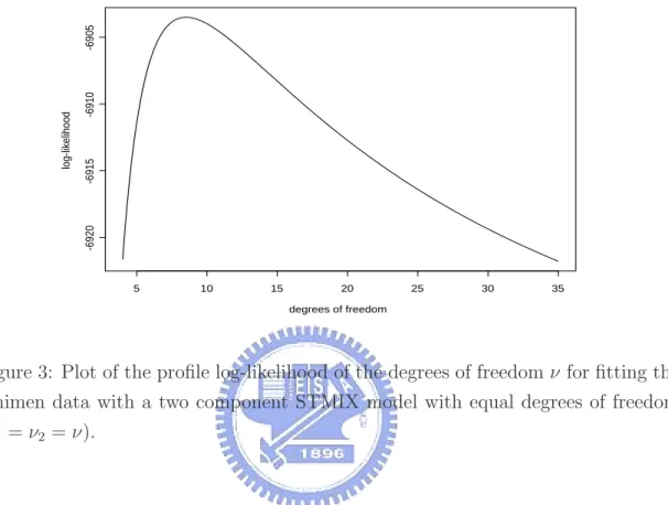
Figure 3: Plot of the profile log-likelihood of the degrees of freedom ν for fitting the bmimen data with a two component STMIX model with equal degrees of freedom

(ν1 = ν2 = ν).

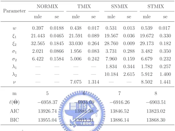
For comparing the fitting results, the ML estimates and the associated information-based standard errors together with the log-likelihood, and AIC and BIC values for NORMIX, TMIX, SNMIX and STMIX models are summarized in Table 1. When comparing these fitted models, we notice that the smaller the AIC and BIC values, the better the fit. It is evidently seen that the STMIX model has the best fitting result. Comparing STMIX with SNMIX, we see that using a heavy-tailed t distribu-tion will reduce the skewness effects. In Figure 3, we plot the profile log-likelihood of the degrees of freedom ν for the STMIX model to illustrate that the SNMIX model is not favorable for this data set since the profile log-likelihood has a significant drop at the peak value of 8.5.

Table 1: ML estimation results for fitting various mixture models on the BMI adult men example.

Parameter NORMIX TMIX SNMIX STMIX

mle se mle se mle se mle se

w 0.397 0.0188 0.438 0.017 0.531 0.013 0.539 0.017 ξ1 21.443 0.0465 21.591 0.089 19.567 0.036 19.672 0.330 ξ2 32.565 0.1845 33.030 0.264 28.760 0.009 29.173 0.182 σ1 2.021 0.0866 1.956 0.083 3.731 0.288 3.482 0.350 σ2 6.422 0.1584 5.006 0.242 7.960 0.159 6.679 0.232 λ1 — — — — 1.834 0.344 1.782 0.257 λ2 — — — — 10.184 2.615 5.912 1.400 ν — — 7.075 1.314 — — 8.502 1.441 m 5 6 7 8 `( ˆΘ) −6958.37 −6934.69 −6916.26 −6903.51 AIC 13926.74 13881.38 13846.52 13823.02 BIC 13955.04 13915.34 13886.14 13868.30

AIC=−2(`( ˆΘ) − m); BIC=−2(`( ˆΘ) − 0.5m log(n)),and m is number of parameters.

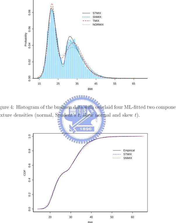
mixture models and display them on a single set of coordinate axes in Figure 4. Based on the graphical visualization, we found that the STMIX fitted density is best followed by the SNMIX fitted density. Both NORMIX and TMIX densities do not fit this data set adequately. For further comparison between the two best models, we display the fitted cdfs for both models along with the empirical cdf of the data set in Figure 5. Again, STMIX provides a closer fit to the data since the fitted STMIX cdf tracks the empirical cdf more closely than does the fitted SNMIX.

15 25 35 45 55 65 BMI 0.00 0.02 0.04 0.06 0.08 Probability STMIX SNMIX TMIX NORMIX

Figure 4: Histogram of the bmimen data with overlaid four ML-fitted two component mixture densities (normal, Student’s t, skew normal and skew t).

20 30 40 50 60 BMI 0.0 0.2 0.4 0.6 0.8 1.0 CDF Empirical STMIX SNMIX

Figure 5: Empirical cdf of the bmimen data together with two superimposed cdfs from the ML-fitted two component SNMIX and STMIX models.

6.

CONCLUDING REMARKS

We have proposed a robust approach to a finite mixture model based on the skew

t distribution, called the STMIX model, which accommodates both asymmetry and

heavy tails jointly that allows practitioners for analyzing data in a wide variety of considerations. We have described a normal-truncated normal-gamma-multinomial hierarchy for the STMIX model and presented some modern EM-type algorithms for ML estimation in a flexible complete-data framework. We demonstrate our approach with a real data set and show that the STMIX model has better performance than the other competitors.

Due to recent advances in computational technology, it is worthwhile to carry out Bayesian treatments via Markov chain Monte Carlo (MCMC) sampling methods in the context of STMIX model. The basic idea is to explore the joint posterior distributions of the model parameters together with latent variables γ and τ , and allocation variables Z when informative priors are employed. Other extensions of the current work include, for example, a generalization of STMIX to multivariate settings (Azzalini and Capitanio 2003; Jones and Faddy 2003) and determination of the number of components in skew t mixtures via reversible jump MCMC (Green 1995; Richardson and Green 1997; Zhang et al. 2004).

APPENDIX

A. Proofs of Eqs. (4), (5), (6) and (7)

Suppose Y∼ ST (ξ, σ2_{, λ, ν), where Z ∼ SN (λ), it has following representation:} Y = ξ + σ√Z

τ, Z ∼ SN (λ), τ ∼ Γ(ν/2, ν/2), Z ⊥ τ.

The condition distribution of Y given τ is

Y |τ ∼ SN (ξ, σ2_{/τ, λ).}

We then have the following result:

E(τn) = Z _∞ 0 τn(ν/2) ν/2 Γ(ν/2) τ ν/2−1_e−ν/2τ_dτ = (ν/2)ν/2 Γ(ν/2) Z _∞ 0 τ(ν+2n)/2−1_e−ν/2τ_dτ = Γ((ν + 2n)/2) Γ(ν/2) ³ν 2 ´_−n . (A.1)

The first four moments of Z are

E(Z) = r 2 πδλ, E(Z 2_{) = 1,} E(Z3) = r 2 πδλ(3 − δ 2 λ), E(Z4) = 3. (A.2)

Applying the double expectation trick, in conjunction of (A.1) and (A.2), we have E(Y ) = E ³ E(Y |τ ) ´ = E(ξ + r 2 πδλ σ √ τ) = ξ + Γ((ν − 1)/2) Γ(ν/2) r ν πδλσ.

It is easy to verify var(Y ) = E(Y − EY )2 = E µ ξ + √σ τZ − ξ − Γ((ν − 1)/2) Γ(ν/2) r ν πδλσ ¶2 = E µ σ2Z2 τ − 2δλσ 2 r ν π Γ((ν − 1)/2) Γ(ν/2) Z √ τ + δ 2 λσ2 ν π( Γ((ν − 1)/2) Γ(ν/2) ) 2 ¶ = σ2_ν µ 1 2 Γ((ν − 2)/2) Γ(ν/2) − δ2 λ π ³Γ((ν − 1)/2) Γ(ν/2) ´₂¶ . Similarly, E(Y − EY )3 _{= σ}3 r ν3 π µ 1 2δλ(3 − δ 2 λ) Γ((ν − 3)/2) Γ(ν/2) −3 2δλ Γ((ν − 1)/2)Γ((ν − 2)/2) Γ(ν/2)2 + 2 πδ 3 λ ³Γ[(ν − 1)/2] Γ[ν/2] ´₃¶ , and E(Y − EY )4 _{= σ}4_ν2 µ 3 4 Γ((ν − 4)/2) Γ(ν/2) − 2 πδλ(3 − δ 2 λ) Γ((ν − 1)/2)Γ((ν − 3)/2) Γ(ν/2)2 +3 πδ 2 λ Γ((ν − 1)/2)2_{Γ((ν − 2)/2)} Γ(ν/2)3 − 3 π2δ 4 λ ³Γ((ν − 1)/2) Γ(ν/2) ´₄¶ .

Let γY and κY denote the skewness and kurtosis, respectively. We have

γY = E(Y − EY )3 ¡ E(Y − EY )2¢3/2 = 1 2 ½ πδλ ¡ 3 − δ2 λ)Γ µ ν − 3 2 ¶ Γ³ν 2 ´₂ −3πδλΓ µ ν − 2 2 ¶ Γ µ ν − 1 2 ¶ Γ³ν 2 ´ + 4δ3 λΓ µ ν − 1 2 ¶₃¾ × ½ π 2Γ µ ν − 2 2 ¶ Γ³ν 2 ´ − δ2 λΓ µ ν − 1 2 ¶₂¾_−3/2 ,

and κY = E(Y − EY )4 ¡ E(Y − EY )2¢2 = ½ 3π2_Γ µ ν − 4 2 ¶ Γ³ν 2 ´₃ − 8πδ2 λ(3 − δ2)Γ µ ν − 3 2 ¶ Γ µ ν − 1 2 ¶ Γ³ν 2 ´₂ +12πδ2 λΓ µ ν − 2 2 ¶ Γ µ ν − 1 2 ¶₂ Γ³ν 2 ´ − 12δ4 λΓ µ ν − 1 2 ¶₄¾ × ½ πΓ µ ν − 2 2 ¶ Γ³ν 2 ´ − 2δ2 λΓ µ ν − 1 2 ¶₂¾₋₂ . B. Proof of Proposition 2

(a) Standard calculation of conditional expectation yields

E(τ | y) = Z _∞ 0 τ f (τ | y)dτ = Z _∞ 0 bτν+12 exp ³ − τ 2(η 2_{+ ν)}´_Φ³_λη√_τ´_dτ = b Γ ³ ν+3 2 ´ ³ η2_+ν 2 ´_(ν+3)/2 Z _∞ 0 γ µ τ |ν + 3 2 , η2_{+ ν} 2 ¶ Φ ³ λη√τ ´ dτ ,

where γ(·|α, β) denotes the density of Γ(α, β) and b is given in (14). By Proposition 1, it suffices to show

E(τ | y) = µ ν + 1 η2_{+ ν} ¶ Tν+3 ³ ληqν+3 η2_+ν ´ Tν+1 ³ ληqν+1 η2_+ν ´.

(b) We first need to show the following:

E³√τφ ¡ λη√τ¢ Φ¡λη√τ¢ | y ´ = Z _∞ 0 √ τφ ¡ λη√τ¢ Φ¡λη√τ¢ f (τ, y) f (y) dτ = (ν/2) ν/2 πσΓ(ν/2)f (y) × Z _∞ 0 τ(ν/2+1)−1_exp µ −τ 2 ³ η2 1 − δ2 λ + ν ´¶ dτ = 1 πσf (y) µ η2 ν(1 − δ2 λ) + 1 ¶_−(ν/2+1) . (B.1)

From (12), the expectation of a truncated normal distribution is given by E(γ | y, τ ) = δλ(y − ξ) + φ¡λη√τ¢ Φ¡λη√τ¢ r 1 − δ2 λ τ σ. (B.2)

Applying the double expectation trick and using (B.1) and (B.2), we get

E(γτ | y) = E ³ τ E(γ | y, τ ) | y ´ = δλ(y − ξ)E(τ | y) + q 1 − δ2 λσE Ã √ τφ ¡ λη√τ¢ Φ¡λη√τ¢ | y ! = δλ(y − ξ)E(τ |y) + p 1 − δ2 λ πf (y) µ η2 ν(1 − δ2 λ) + 1 ¶_−(ν/2+1) .

(c) Similarly, it is easy to verify that

E(γ2 _{| y, τ ) = δ}2 λ(y − ξ)2+ (1 − δ2 λ)σ2 τ + σδλ(y − ξ) r 1 − δ2 λ τ φ¡λη√τ¢ Φ¡λη√τ¢. (B.3)

Using (B.1) and (B.3), and the double expectation trick as before gives

E(γ2τ | y) = δ_λ2(y − ξ)2E(τ |y) + (1 − δ_λ2)σ2 +δλ(y − ξ) p 1 − δ2 λ πfY(y) µ η2 ν(1 − δ2 λ) + 1 ¶_−(ν/2+1) .

(d) From (13), it is true that

d dν Z _∞ 0 f (τ | y)dτ = d dν Z _∞ 0 bτ(ν−1)/2_exp³₋τ 2(η 2_{+ ν)}´_Φ(λη√_{τ )dτ = 0.}

By Leibnitz’s rule, we can get log³η 2_{+ ν} 2 ´ + µ ν + 1 η2_{+ ν} ¶ − DG(ν + 1 2 ) − 1 Tν+1(M) Z _M −∞ gν(x)tν+1(x)dx +λ(ν + 1)−12η(η2− 1)(η2+ ν)− 3 2 tν+1(M) Tν+1(M) + E(log τ | y) − E(τ | y) = 0. Hence E¡log(τ )|y¢ = DG µ ν + 1 2 ¶ − log³η 2_{+ ν} 2 ´ + ν + 1 η2_{+ ν}  Tν+3 ³ M q ν+3 ν+1 ´ Tν+1(M) − 1   + λη(η 2_{− 1)} p (ν + 1)(ν + η2₎3 tν+1(M) Tν+1(M) + 1 Tν+1(M) Z _M −∞ gν(x)tν+1(x)dx.

C. The PX-EM Algorithm

The method of parameter-expansion EM, PX-EM, introduced by Liu, Rubin and Wu (1998), shares the simplicity and stability of ordinary EM, but has a faster rate of convergence. PX-EM algorithm accelerates EM algorithm since its E-step execute a more efficient analysis. PX-EM is to perform a covariance adjustment to correct the analysis of the M step, capitalizing on extra information captured in the imputed complete data.

PX-EM expands the complete data model f (ycom|θ) to a larger model, fX(ycom|Θ),

with Θ = {θ∗, α}, and α is an auxiliary scale parameter whose value is fixed at α0

in the original model. If the auxiliary parameter α equal to 1, {θ} = {θ∗}.

And then, we want to compare ECM algorithm with PX-EM algorithm for ML estimation of skew t distribution.

Model O: Y | γ, τ ∼ N µ ξ + δλγ, 1 − δ2 λ τ σ 2 ¶ , γ | τ ∼ T N µ 0,σ2 τ ; [0, ∞) ¶ , τ ∼ Γ(ν/2, ν/2),

and θ = (ξ, σ2_{, λ, ν) is the parameter of the stew t distribution in ECM algorithm.}

The results of ECM algorithm are referred to Section 3.

We now derive this modified ECM using PX-EM, and want to adjust current estimates by expanding the parameter:

Model X: Y | γ, τ ∼ N µ ξ∗+ δλγ, 1 − δ2 λ τ σ 2 ∗ ¶ , γ | τ ∼ T N µ 0,σ 2 ∗ τ ; [0, ∞) ¶ , τ = αχ 2 ν ν ∼ Γ(ν/2, ν/2),

And

(ξ, σ2_{, λ, ν) = R{(ξ}

∗, σ2∗, λ, ν, α)} = (ξ∗, σ∗2/α, λ, ν)

where R is the reduction function from the expanded parameter space to the original parameter space.

Applying routine algebraic manipulations leads to the following CM-step for updating α ˆ α(k+1) _{= n}−1 n X j=1 ˆ s(k)_1j

the application of the reduction function in the PX-EM algorithm leads to adjust-ments in the estimates of σ2_{and ν, which can be obtained by replacing the CM-steps}

2 and 4 in the previous EM algorithm with the following two PX.CM steps: PX.CM-step2: ˆ σ2(k+1) = P_n j=1 ³ ˆ s(k)_1j (yj − ˆξ(k+1))2− 2ˆδ(k)λ sˆ (k) 2j (yj − ˆξ(k+1)) + ˆs(k)3j ´ 2(1 − ˆδ2(k) λ ) P_n j=1sˆ (k) 1j . PX.CM-step4: log à nν 2Pn_j=1sˆ(k)_1j ! − DG(ν 2) + 1 n n X j=1 ˆ s(k)_4j = 0.

In the same way, under stew t mixture model, applying routine algebraic manip-ulations leads to the following CM-step for updating αi

ˆ α(k+1)_i = n X j=1 ˆ s(k)_1ij/ n X j=1 ˆ z_ij(k)

the application of the reduction function in the PX-EM algorithm leads to adjust-ments in the estimates of σ2

iand νi, which can be obtained by replacing the CM-step

3 and 5 in the previous EM algorithm with the following two PX.CM step: PX.CM-step3: ˆ σi2(k+1) = P_n j=1ˆs (k) 1ij(yj− ˆξi (k+1) )2_{− 2 ˆδ} i (k)P_n j=1ˆs (k) 2ij(yj− ˆξi (k+1) ) +Pn_j=1sˆ(k)_3ij 2(1 − ˆδi 2(k) )Pn_j=1sˆ(k)_1ij .

PX.CM-step5: log³νi P_n j=1zˆ (k) ij 2Pn_j=1sˆ(k)_1ij ´ − DG³νi 2 ´ + P_n j=1sˆ (k) 4ij P_n j=1zˆ (k) ij = 0.

REFERENCES

Azzalini, A. (1985), “A Class of Distributions Which Includes the Normal Ones,”

Scandinavian Journal of Statistics, 12, 171-178.

Azzalini, A. (1986), “Further Results on a Class of Distributions Which Includes the Normal Ones,” Statistica 46, 199-208.

Azzalini, A., and Capitaino, A. (2003), “Distributions Generated by Perturbation of Symmetry With Emphasis on a Multivariate Skew t-Distribution,” Journal

of the Royal Statistical Society. Ser. B, 65, 367-389.

Basord, K. E., Greenway D. R., McLachlan G. J., and Peel D. (1997), “Standard Errors of Fitted Means Under Normal Mixture,” Computational Statistics, 12, 1-17.

Dempster, A. P., Laird, N. M., and Rubin, D. B. (1977), “Maximum Likelihood from Incomplete Data via the EM Algorithm (with discussion),” Journal of

the Royal Statistical Society. Ser. B, 39, 1-38.

Flegal, K. M., Carroll, M. D., Ogden, C. L., and Johnson, C. L. (2002), “Prevalence and Trends in Obesity among US Adults, 1999-2000,” Journal of the American

Fraley, C, and Raftery, A. E. (2002), “Model-Based Clustering, Discriminant Analy-sis, and Density Estimation,” Journal of the American Statistical Association, 97, 611-631.

Green, P. J., (1995), “Reversible Jump MCMC Computation and Bayesian Model Determination,” Biometrika, 82, 711-732.

Henze, N. (1986), “A Probabilistic Representation of the Skew-Normal Distribu-tion,” Scandinavian Journal of Statistics, 13, 271-275.

Jones, M. C., and Faddy, M. J. (2003), “A Skew Extension of the t-Distribution, With Applications,” Journal of the Royal Statistical Society. Ser. B, 65, 159-174.

Lin, T. I., Lee, J. C., and Ni, H. F. (2004), “Bayesian Analysis of Mixture Modelling Using the Multivariate t Distribution,” Statistics and Computing, 14, 119-130. Lin, T. I., Lee, J.C., and Yen, S. Y. (2006), “Finite Mixture Modelling Using the

Skew Normal Distribution,” Statistica Sinica (To appear).

Liu, C. H., and Rubin, D. B. (1994), “The ECME Algorithm: a Simple Extension of EM and ECM With Faster Monotone Convergence,” Biometrika, 81, 633-648. Liu, C. H., Rubin, D. B., and Wu, Y. (1998). “Parameter Expansion to Accelerate

EM: the PX-EM Algorithm,” Biometrika, 85, 755-770.

McLachlan, G. J. and Basord, K. E. (1988), Mixture Models: Inference and

Appli-cation to Clustering, Marcel Dekker, New York.

Meng, X. L., and Rubin, D. B. (1993), “Maximum Likelihood Estimation via the ECM Algorithm: A General Framework,” Biometrika, 80, 267-78.

Peel, D., and McLachlan, G.J. (2000), “Robust Mixture Modeling Using the t Distribution,” Statistics and Computing 10, 339-348.

Richardson, S., and Green, P. J. (1997), “On Bayesian Analysis of Mixtures With an Unknown Number of Components (with discussion),” Journal of the Royal

Statistical Society. Ser. B, 59, 731-792.

Shoham, S. (2002). “Robust Clustering by Deterministic Agglomeration EM of Mixtures of Multivariate t-Distributions,” Pattern Recognition, 35, 1127-1142. Shoham, S., Fellows, M. R., and Normann R. A. (2003), “Robust, Automatic Spike Sorting Using Mixtures of Multivariate t-Distributions,” Journal of

Neuro-science Methods, 127, 111-122.

Titterington, D. M., Smith, A. F. M. and Markov, U. E. (1985), Statistical Analysis

of Finite Mixture Distributions, Wiely, New York.

Wang, H. X., Zhang, Q. B., Luo, B., and Wei, S. (2004), “Robust Mixture Mod-elling Using Multivariate t Distribution With Missing Information”, Pattern

Recognition Letter, 25, 701-710.

Zacks, S. (1971), The Theory of Statistical Inference, Wiley, New York.

Zhang, Z., Chan, K. L., Wu, Y., and Cen, C. B. (2004), “Learning a Multivari-ate Gaussian Mixture Model With the Reversible Jump MCMC Algorithm,”