Multi-response robust design by principal component analysis

This article was downloaded by: [National Chiao Tung University 國立交通大

學]

On: 01 May 2014, At: 02:30

Publisher: Routledge

Informa Ltd Registered in England and Wales Registered Number: 1072954

Registered office: Mortimer House, 37-41 Mortimer Street, London W1T

3JH, UK

Total Quality Management

Publication details, including instructions for

authors and subscription information:

http://www.tandfonline.com/loi/ctqm19

Multi-response robust design

by principal component

analysis

Chao-Ton Su & Lee-Ing Tong

Published online: 25 Aug 2010.

To cite this article: Chao-Ton Su & Lee-Ing Tong (1997) Multi-response robust design

by principal component analysis, Total Quality Management, 8:6, 409-416, DOI:

10.1080/0954412979415

To link to this article:

http://dx.doi.org/10.1080/0954412979415

PLEASE SCROLL DOWN FOR ARTICLE

Taylor & Francis makes every effort to ensure the accuracy of all

the information (the “Content”) contained in the publications on our

platform. However, Taylor & Francis, our agents, and our licensors

make no representations or warranties whatsoever as to the accuracy,

completeness, or suitability for any purpose of the Content. Any opinions

and views expressed in this publication are the opinions and views of

the authors, and are not the views of or endorsed by Taylor & Francis.

The accuracy of the Content should not be relied upon and should be

independently verified with primary sources of information. Taylor and

Francis shall not be liable for any losses, actions, claims, proceedings,

demands, costs, expenses, damages, and other liabilities whatsoever

or howsoever caused arising directly or indirectly in connection with, in

relation to or arising out of the use of the Content.

This article may be used for research, teaching, and private study

purposes. Any substantial or systematic reproduction, redistribution,

reselling, loan, sub-licensing, systematic supply, or distribution in any form

to anyone is expressly forbidden. Terms & Conditions of access and use can

be found at

http://www.tandfonline.com/page/terms-and-conditions

TO TA L Q UALITY M AN AGEM EN T, VO L. 8, N O. 6, 1997, 409 ± 416

M ulti-response robust design by principal

com ponent analysis

C

HAO

-T

ON

S

U

& L

EE

-I

NG

T

ONG

Department of Industrial Engineering and M anagement, N ational Chiao Tung U niversity, Hsinchu, Taiwan, ROC

Abstract M ost previous Taguchi method applications have only addressed a single-response

problem. However, more than one correlated response nor mally occurs in a manufactured product. The multi-response problem has received only limited attention. In this work, we propose an eŒective procedure on the basis of principal com ponent analysis (PCA ) to optimize the m ulti-response problems in the Taguchi method. W ith the PC A , a set of original responses can be transform ed into a set of uncor related components. Therefore, the con¯ ict for deter mining the optim al settings of the design parameters for the m ulti-response problems can be reduced. Two case studies are evaluated, indicating that the proposed procedure yields a satisfactor y result.

Introd uction

Robust design is an engineering m ethod of quality im provem ent that seeks to obtain a lowest cost solution to the product design speci® cation based on the custom er’ s requirem ents. Th e Taguchi m ethod, wh ich com bines the experimental design techniques with quality loss considerations, is the conventional approach to achieve robustness. This m ethod can only be used in a single-response case; it cannot be used to optim ize a m ulti-response problem . However, a custom er norm ally considers m ore than one quality characteristic in m ost m anufactured products and the quality characteristics are usually correlated. Engineering judgem ent has, up until now, been used prim arily to optim ize th e m ulti-response problem in the Taguchi m ethod (Phadke, 1989). U nfortunately, an engineer’s judgem ent increases the uncertainty during the decision-m aking process. A nother approach to solve this problem entails assigning a weight for each response (H ung, 1990; Shiau, 1990; Tai et al., 1992). Neverth eless, determ ining a de® nite weight for each response in an actual case still rem ains di cult. Another m ethod employs the regression technique (Logothetis & H aigh, 1988; Pignatiello, 1993). However, such an approach increases the com putational process com plex-ity, and the possible correlations am ong th e responses m ay still not be considered. In addition, a factor which is signi® cant in a single-response case m ay not be signi® cant when considered in a m ulti-response case. Therefore, a m ore eŒective approach is required to solve this com plicated problem .

In this work, we propose a system atic procedure via principal com ponent analysis (PC A) to optim ize the m ulti-response production process. By using PC A, a set of original responses is transform ed into a set of uncorrelated com ponents so that the optim al factor/level com bination can be found. Th e proposed procedure includes a series of steps capable of

0954 ± 4127 /97/060409-0 8 $7.00 € 199 7 Carfax Publishing Ltd

410 C .-T. SU & L.-I. TO NG

decreasing the uncertainty in engineering judgem ent when the Taguchi m ethod is applied. Th is work addresses only the static quality characteristic problem , in which the desired response value is ® xed.

PC A

Pearson and Hotelling (1933) ® rst introduced PC A. PC A is used to explain the variance± covariance structure through the linear com binations of the original variables. Assum e that there are p com ponents to represent the system variability. By using PC A, th is variability can be explained by a sm all num ber, k(k< p), of the principal com ponents, i.e. k principal

com ponents will account for m ost of the variance in the original p variables. Let Y1, Y2, . . . ,

Yp be a set of variables. Through the PC A, we have the following uncorrelated linear

com binations: X 15 a11Y1+ a12Y2+ . . .+ a1pYp X 25 a21Y1+ a22Y2+ . . .+ a2pYp

:

k1+ a2k2+ . . .+ a2kp5 1. Further, X 1is called the ® rst principal com ponent,X 2is called

the second principal com ponent and so on. Th e coe cients of the kth com ponent are the elem ents of the eigenvector corresponding to the kth largest eigenvalues. The option of perform ing the PCA is available on SAS and SPSSX .

M ore than one correlated quality characteristic is usually considered in a m anufactured product. PC A is an eŒective m eans of determ ining a sm all num ber of constructs which account for the m ain sources of variation in such a set of correlated quality characteristics.

Proposed p rocedure

In this section, an eŒective procedure is developed to transform a set of responses into a set of uncorrelated com ponents such that the optim al conditions in the param eter design stage for the m ulti-response problem can be determ ined. Assum e that we have p responses. The proposed procedure is described in th e following.

Step 1: Compute the quality loss for each response. Let Lijbe the quality loss for ith response

at jth trial. Lijcan be com puted on the basis of Taguchi’ s loss function.

Step 2: N or malize Lij. To reduce the variability, the scale of the quality loss for each response

is norm alized. Lijis transform ed into Yij(0< Yij< 1) by using the following form ula:

Yij5

L+i 2 Lij

L+i 2 L2i

where Yij5 the normalized quality loss for ith response at jth trial; L+i 5 max{Li1,

Li 2, . . . , Li j} ; L2i 5 min{Li1, Li 2, . . . , Lij}.

Step 3: Perfor m the PC A on the basis of the com puted data, Yij.

Step 4: D eter mine the num ber of principal components, k, and compute

X kj5

R

i5 1

akiYij

M ULTI-R ESP O N SE RO BU ST DE SIG N 411

where ak1, ak2, . . . , akp are th e elem ents of the eigenvector corresponding to the kth largest

eigenvalue.X can be considered as a m ulti-response perform ance index, which can be used to determ ine th e optim al conditions. Based on Kasier’ s (1960) study, the com ponents with eigenvalue greater than 1 are chosen to replace the original responses for further analysis.

Step 5: D eterm ine the optimal factor/level com bination. The larger the X value implies the better the product quality. If k5 1, the factor eŒects can be estimated and the optimal control factors and their levels determ ined on the basis of a singleX value. If k> 1, trade-oŒs m ight be necessar y to select a feasible solution.

Illustrations

Th is section dem onstrates the eŒectiveness of the proposed procedure by using tw o case studies.

Case study 1

Th is case study involves improving a hard disk drive’ s quality. The Industrial Technology Research Institute, Taiwan, perform ed the case study. In this study, an experiment was perform ed to determ ine the eŒects of design param eters on the responses. Optim al settings could, it was hoped, be found such that a low variability for the responses could be achieved. Th e four desired responses are:

PW: 50% pulse width (sm aller-the-better);

H FA : high-frequency am plitude (larger-the-better); OW: over write (larger-the-better);

PS: peak shift (sm aller-the-better).

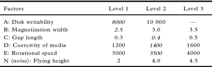
In the experim ent, ® ve controllable factors were selected for optim ization. Table 1 lists th ese factors and th eir alternative levels. The standard array L18 was selected for the experiment.

Table 2 sum m arizes the data for 18 exp eriments.

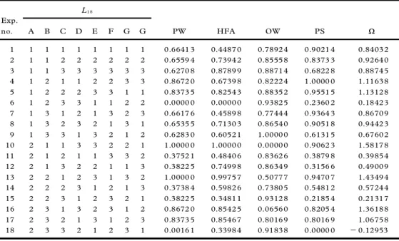
W hen the proposed procedure is applied in th is case study, the quality loss for each response is ® rst com puted and norm alized, as shown in Table 3. Next, the PC A is perform ed on these norm alized data using SAS. Table 4 lists the eigenvalues. Based on Kasier’ s criterion, the ® rst principal com ponent is chosen to represent the original four responses. The eigenvector for the ® rst largest eigenvalue is [0.59716, 0.50583, 2 0.3296, 0.52883]. Consequently, we have

X 1j5 0.59716Y1j+ 0.50583Y2j2 0.3296Y3j+ 0.52883Y4j

Table 1. Factors and their levels (case study 1)

Factors Level 1 Level 2 Level 3

A: Disk writability 8000 10 000 Ð

B: M agnetization width 2.5 3.0 3.5

C: Gap length 0.3 0.4 0.5

D: Coercivity of media 1200 1400 1600

E: Rotational speed 3000 3500 4000

N (noise): Flying height 2 4.0 4.5

Starting levels are identi® ed by italics.

412 C .-T. S U & L.-I. TO N G

Table 2. Data summar y by experiment (case study 1)

Factors PW H FA OW PS Exp. no. A B C D E F G H N1 N2 N1 N2 N1 N2 N1 N2 1 1 1 1 1 1 1 1 1 63.5 66.0 286.7 257.6 2 32.2 2 30.1 10.9 12.0 2 1 1 2 2 2 2 2 2 64.2 66.0 343.0 310.6 2 34.8 2 33.3 11.6 13.0 3 1 1 3 3 3 3 3 3 65.6 67.0 381.1 354.4 2 36.2 2 35.3 13.6 14.7 4 1 2 1 1 2 2 3 3 54.5 56.6 328.1 295.4 2 33.5 2 31.5 9.2 10.8 5 1 2 2 2 3 3 1 1 56.2 57.8 368.3 333.0 2 36.2 2 34.9 10.2 11.2 6 1 2 3 3 1 1 2 2 87.5 89.3 234.3 213.5 2 40.0 2 38.4 17.8 19.1 7 1 3 1 2 1 3 2 3 63.6 66.1 288.0 259.2 2 31.7 2 29.5 10.1 11.8 8 1 3 2 3 2 1 3 1 64.3 66.1 335.8 304.9 2 35.2 2 33.9 10.7 12.1 9 1 3 3 1 3 2 1 2 65.6 66.9 312.7 282.8 2 43.7 2 46.5 14.4 15.4 10 2 1 1 3 3 2 2 1 47.7 49.5 451.0 393.8 2 15.6 2 22.3 11.0 11.8 11 2 1 2 1 1 3 3 2 74.9 77.0 291.6 263.0 2 33.6 2 32.6 16.3 17.9 12 2 1 3 2 2 1 1 3 74.9 76.5 346.8 312.4 2 35.1 2 33.8 16.9 18.6 13 2 2 1 2 3 1 3 2 47.7 49.5 447.9 393.8 2 25.8 2 22.3 10.0 11.6 14 2 2 2 3 1 2 1 3 75.0 77.0 312.8 280.5 2 29.7 2 28.9 14.6 16.5 15 2 2 3 1 2 3 2 1 74.9 76.5 271.9 245.4 2 38.4 2 38.9 18.0 19.2 16 2 3 1 3 2 3 1 2 54.5 56.6 385.2 336.7 2 20.4 2 17.2 11.6 13.4 17 2 3 2 1 3 1 2 3 56.2 57.8 378.7 341.5 2 35.6 2 34.6 12.1 13.4 18 2 3 3 2 1 2 3 1 87.4 89.3 270.6 244.6 2 38.5 2 37.0 19.4 21.3

Table 3. Normalized data and X values (case study 1)

L1 8 Exp. no. A B C D E F G G PW HFA OW PS X 1 1 1 1 1 1 1 1 1 0.6641 3 0.4487 0 0.7892 4 0.9021 4 0.8403 2 2 1 1 2 2 2 2 2 2 0.6559 4 0.7394 2 0.8555 8 0.8373 3 0.9264 0 3 1 1 3 3 3 3 3 3 0.6270 8 0.8789 9 0.8871 4 0.6822 8 0.8874 5 4 1 2 1 1 2 2 3 3 0.8672 0 0.6739 8 0.8222 4 1.0000 0 1.1163 8 5 1 2 2 2 3 3 1 1 0.8373 5 0.8254 3 0.8835 2 0.9551 5 1.1312 8 6 1 2 3 3 1 1 2 2 0.0000 0 0.0000 0 0.9382 5 0.2360 2 0.1842 3 7 1 3 1 2 1 3 2 3 0.6617 6 0.4589 8 0.7744 4 0.9364 3 0.8670 9 8 1 3 2 3 2 1 3 1 0.6535 5 0.7130 3 0.8654 0 0.9051 8 0.9442 3 9 1 3 3 1 3 2 1 2 0.6283 0 0.6052 1 1.0000 0 0.6131 5 0.6760 2 10 2 1 1 3 3 2 2 1 1.0000 0 1.0000 0 0.0000 0 0.9062 3 1.5817 8 11 2 1 2 1 1 3 3 2 0.3752 1 0.4840 6 0.8362 6 0.3879 8 0.3985 4 12 2 1 3 2 2 1 1 3 0.3822 5 0.7499 8 0.8634 9 0.3156 6 0.4900 9 13 2 2 1 2 3 1 3 2 1.0000 0 0.9975 7 0.5077 7 0.9470 7 1.4349 4 14 2 2 2 3 1 2 1 3 0.3738 4 0.5982 6 0.7380 5 0.5481 2 0.5724 4 15 2 2 3 1 2 3 2 1 0.3822 5 0.3481 1 0.9312 8 0.2185 4 0.2131 7 16 2 3 1 3 2 3 1 2 0.8672 0 0.8542 5 0.0656 0 0.8205 4 1.3618 8 17 2 3 2 1 3 1 2 3 0.8373 5 0.8546 7 0.8016 9 0.8016 9 1.0675 8 18 2 3 3 2 1 2 3 1 0.0016 1 0.3398 4 0.9183 8 0.0000 0 2 0.12953

where Yj1, Yj2, Yj3 and Yj4represent the norm alized quality loss for the responses PW, H FA ,

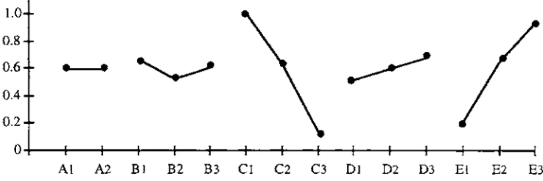
OW and PS at jth trial respectively. TheX values are com puted and listed in the last colum n of Table 3. Table 5 sum m arizes the m ain eŒects on X and Fig. 1 plots their corresponding factor eŒects. The controllable factors on X value in order of signi® cance are: C, E, D, B and A . The larger the X value implies the better the quality. C onsequently, the optim al condition can be set as A1B1C1D3E3.

M ULTI-R ESP O N SE RO BU ST DE SIG N 413

Table 4. Eigenvalues for the pr incipa l components (case study 1)

Principal component Eigenvalue

First 2.93478

Second 0.68014

Third 0.33771

Fourth 0.04736

Table 5. Main eŒects on X (case study 1)

Factor Level 1 Level 2 Level 3 M ax2 min

A 0.5950 0.5926 Ð 0.0024

B 0.6623 0.5163 0.6027 0.1460

C 1.0108 0.6380 0.1325 0.8783

D 0.5147 0.5900 0.6771 0.1624

E 0.2029 0.6474 0.9311 0.7282

Figure 1. Factor eŒects on X (case study 1).

This case study is also analyzed by the Taguchi’ s approach. The tentative optim um setting can be separately m ade in the following:

PW: A2B1C1D1E3

H FA : A2B1C1D3E3

OW: A1B2C3D1E1

PS: A1B3C1D2E3

Th ese results dem onstrate th at diŒerent levels of the sam e factor can be optim um for diŒerent responses. As a result, th e decision-m aking process is di cult. B ased on the signi® cance of the factor eŒects and the engineering judgem ent, the optim al condition is set as A1B1C1D1E3.

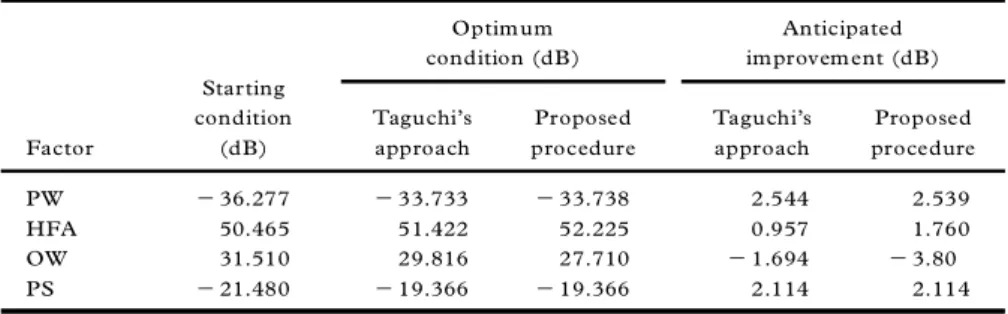
To predict the anticipated improvem ents under the chosen optim um conditions, the signal to noise (SN ) ratios for these four responses are predicted using the additive m odel. Table 6 displays the com putations. This table reveals that no signi® cant diŒerence arises in the eŒectiveness between the proposed procedure and Taguchi’ s approach. H owever, the proposed procedure can be considered as a m ore convenient approach than Taguchi’ s m ethod in the m ulti-response case, owing to the fact that the decision-m aking’ s com plexity is reduced.

414 C .-T. SU & L.-I. TO NG

Table 6. Prediction of SN ratios using the additive model (case study 1)

Optim um Anticipated

condition (dB) improvement (dB)

Starting

condition Taguchi’ s Proposed Taguchi’s Proposed

Factor (dB) approach procedure approach procedure

PW 2 36.277 2 33.733 2 33.738 2.544 2.539

HFA 50.465 51.422 52.225 0.957 1.760

OW 31.510 29.816 27.710 2 1.694 2 3.80

PS 2 21.480 2 19.366 2 19.366 2.114 2.114

Case study 2

Phadke (1989) considered a case study to improve a polysilicon deposition process. This study was conducted by Peter Hey in 1984. Six controllable factors were identi® ed: deposition tem perature (A), deposition pressure (B), nitrogen ¯ ow (C), silane ¯ ow (D ), setting tim e (E) and cleaning m ethod (F). A ll the factors were studied at three levels each. The L18orthogon al

array was used and factors A± F were assigned to colum ns 2, 3, 4, 5, 6 and 8 respectively. Th e quality characteristics of interest were the surface defects (sm aller-th e-better), the thickness (nom inal-the-best) and the deposition rate (larger-the-better). The target value in the study for the thickness of polysilicon layer was 3600 AÊ. Nine observations were taken for each trial run. The starting condition was set as A2B2C1D3E1F1. Th e optim um condition

chosen from the experim ental data by Phadke was A1B2C1D3E2F2.

The above case is analyzed again by the proposed procedure. The quality loss for each response is com puted and norm alized as shown in Table 7. Next, the PC A is perform ed on these norm alized data using SAS. Table 8 lists the eigenvalues. The ® rst principal com ponent

Table 7. Nor malized data and X values (case study 2)

L1 8

Exp. Surface Deposition

no. A B C D E F G H defects Thickness rate X

1 1 1 1 1 1 1 1 1 1.0000 0 0.9822 7 1.0000 0 1.7201 0 2 1 1 2 2 2 2 2 2 0.9996 6 0.9847 2 0.9131 5 1.6716 0 3 1 1 3 3 3 3 3 3 0.9979 3 0.9858 0 0.8846 3 1.6546 6 4 1 2 1 1 2 2 3 3 0.9999 8 0.9990 8 0.9159 6 1.6811 9 5 1 2 2 2 3 3 1 1 0.8867 6 0.5015 8 0.6060 0 1.1643 7 6 1 2 3 3 1 1 2 2 0.8945 6 0.9675 5 0.8278 3 1.5488 3 7 1 3 1 2 1 3 2 3 0.9386 2 0.4969 4 0.5653 9 1.1705 7 8 1 3 2 3 2 1 3 1 0.0688 9 0.6406 5 0.1249 9 0.4615 6 9 1 3 3 1 3 2 1 2 0.5879 0 0.9425 0 0.0000 0 0.8734 8 10 2 1 1 3 3 2 2 1 1.0000 0 0.8592 2 0.9688 7 1.6355 2 11 2 1 2 1 1 3 3 2 1.0000 0 0.9940 4 0.9854 2 1.7181 5 12 2 1 3 2 2 1 1 3 0.9807 2 0.9923 3 0.8992 4 1.6561 2 13 2 2 1 2 3 1 3 2 0.9945 3 0.9599 4 0.7994 2 1.5900 1 14 2 2 2 3 1 2 1 3 0.9997 2 1.0000 0 0.8555 0 1.6469 8 15 2 2 3 1 2 3 2 1 0.8348 0 0.9906 6 0.7860 5 1.5007 2 16 2 3 1 3 2 3 1 2 0.9999 7 0.9578 0 0.5622 7 1.4567 0 17 2 3 2 1 3 1 2 3 0.1066 9 0.5643 0 0.1631 4 1.4651 8 18 2 3 3 2 1 2 3 1 0.0000 0 0.0000 0 0.3735 4 0.2134 2

M ULTI-R ESP O N SE RO BU ST DE SIG N 415

Table 8. Eigenvalues for the pr incipa l components (case study 2)

Principal component Eigenvalue

First 2.37892

Second 0.46894

Third 0.15215

is chosen to represent the original three responses. Th e eigenvector for th e ® rst largest eigenvalue is [0.61559, 0.54279, 0.57134]. As a result, we have

X 1j5 0.61559Y1j+ 0.54279Y2j+ 0.57134Y3j

where Yj1, Yj2and Yj3represent the norm alized quality loss for th e surface defects, th ickness

and deposition rate at jth trial respectively. The X values are com puted and listed in the last colum n of Table 7. The factor eŒects on X can be obtained and the optim al conditions can therefore be set as A1B1C3D2E3F2.

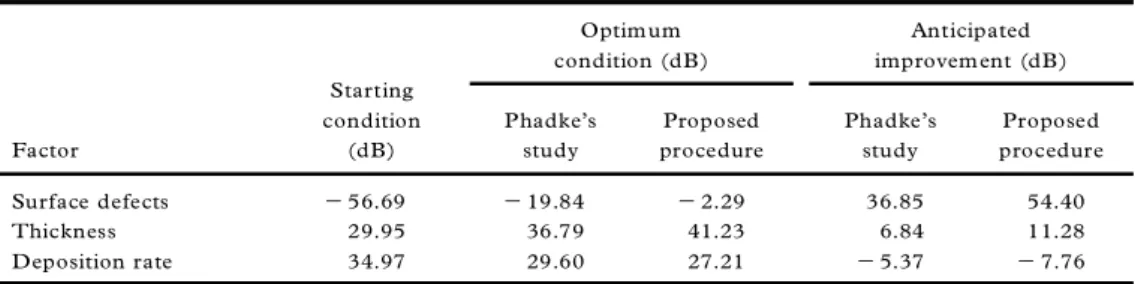
To predict the anticipated improvem ents under the chosen optim um conditions, the SN ratios for surface defects, thickness and deposition rate are predicted using the additive m ode. Table 9 displays the com putations for Phadke’ s study and proposed analyses. According to this table, an improvem ent in surface defects for th e proposed procedure analysis is equal to [(2 2.29)2 (2 56.69)]5 54.40 dB, which is larger than the improvement in Phadke’ s study of 36.85 dB. Similarly, the improvem ent in thickness uniform ity for the proposed procedure analysis is better than that of Phadke’ s study. A slight reduction occurs in the deposition rate for the proposed procedure. C onsequently, in this case study, the proposed procedure can be considered as a m ore eŒective approach than Phadke’ s study (based on an engineer’ s judgem ent) in the m ulti-response problem .

Conclusions

A procedure has been proposed in this study to achieve th e optim ization of m ulti-response problem s in the Taguchi m ethod. By using PC A, a set of (correlated) responses is transform ed into a set of a sm all num ber of uncorrelated com ponents. Principal com ponents reduce the num ber of dimensions and decrease the com plexity of the m ulti-response problem s. Accordingly, based on these uncorrelated com ponents, the optim al conditions in the par-am eter design stage can be easily chosen in an objective m anner. In addition, two case studies dem onstrate the eŒectiveness of the proposed procedure.

Table 9. Prediction of SN ratios using the additive model (case study 2)

Optim um Anticipated

condition (dB) improvement (dB)

Starting

condition Phadke’ s Proposed Phadke’ s Proposed

Factor (dB) study procedure study procedure

Surface defects 2 56.69 2 19.84 2 2.29 36.85 54.40

Thickness 29.95 36.79 41.23 6.84 11.28

Deposition rate 34.97 29.60 27.21 2 5.37 2 7.76

416 C .-T. SU & L.-I. TO NG

References

HOTELLING, H . (1933 ) Analysis of a complex of statistical variables into principal components, Journal of

Education al Psychology, 24, pp. 417 ± 441, 498 ± 520 .

HUNG, C.H. (1990) A Cost-eŒective M ulti-purpose OŒ-line Quality Control for Semiconductor Manufacturing,

Master’ s thesis, National Chiao Tung University, Taiwan.

KAISER, H .F. (1960 ) The application of electronic computers to factor analysis, Educational and Psychological

Measurement, 20, pp. 141 ± 151 .

LOGOTHETIS, N. & HAIGH, A. (1988 ) Characterizing and optimizing multi-response processes by the Taguchi

method, Quality and Reliability Engineering Inter national, 4, pp. 159 ± 169.

PHADKE, M.S. (1989) Quality Engineering Using Robust Design (Englewood CliŒs, NJ, Prentice Hall).

PIGNATIELLO, J.J. JR (1993 ) Strategies for robust multiresponse quality engineering, IIE Transactions, 25,

pp. 5 ± 15.

SHIAU, G.H. (1990 ) A study of the sintering properties of iron ores using the Taguchi’ s parameter design,

Journal of the Chinese Statistical A ssociation, 28, pp. 253 ± 275.

TAI, C.Y., CHEN, T.S. & WU, M.C. (1992 ) An enhanced Taguchi method for optimizing SM T processes,

Journal of Electronics Manufactur ing, 2, pp. 91 ± 100.