堅硬土層侵入回填土對擋土牆主動土壓力之影響

國立交通大學

土木工程學系碩士班

碩士論文

堅硬土層侵入回填土對擋土牆主動土壓力之

影響

Active Earth Pressure on Retaining Walls with Intrusion

of a Stiff Interface into Backfill

研究生 : 鄭詠誠

指導教授 : 方永壽 博士

堅硬土層侵入回填土對擋土牆主動土壓力之

影響

Active Earth Pressure on Retaining Walls with Intrusion

of a Stiff Interface into Backfill

研究生：鄭詠誠 Student：Yung-Chen Zheng

指導教授：方永壽 博士 Advisor：Dr. Yung-Show Fang

國立交通大學土木工程學系碩士班

碩士論文

A Thesis

Submitted to the Department of Civil Engineering

College of Engineering

National Chiao Tung University

in Partial Fulfillment of the Requirements

for the Degree of

Master of Engineering in

Civil Engineering

September 2007

Hsinchu, Taiwan, Republic of China

中華民國九十七年九月

堅硬土層侵入回填土對擋土牆主動土

壓力之影響

研究生 : 鄭詠誠 指導教授 : 方永壽 博士

國立交通大學土木工程學系碩士班

摘要

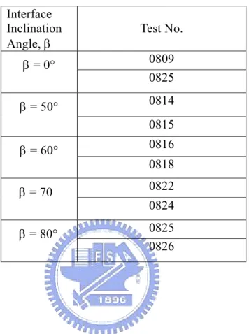
本論文探討堅硬土層入侵回填土對擋土牆主動土壓力之影響。本研究以氣乾之渥太華 砂作為回填土，回填土高0.5 公尺。量測於鬆砂(Dr = 35%)狀態下作用於剛性榜土牆的側 向土壓力。本研究利用國立交通大學模型擋土牆設備來探討堅硬以不同界面傾角　侵入回 填土對擋土牆主動土壓力影響。為了模擬堅硬的土層界面，本研究設計並建造一片鋼製傾 斜界面板，及其支撐系統。本研究共執行五種堅硬界面傾角β = 0o 、50o 、60o 、70o 與 80o 五 種實驗。依擋土牆砂實驗結果，本研究獲得以下幾項結論。 1. 當岩石界面傾角β = 0o 時，其主動土壓力係數Ka,h 與 Coulomb 解相吻合，其主動合力約 作用於距擋土牆底部0.33H 處。 2. 在岩石界面傾角 45o、60o、70o與 80o狀況下，側向土壓力隨深度的增加而呈非線性分 布，所獲得的側向土壓力低於Jaky 解，側向土壓力隨界面傾角的增加而減少。 3. 當界面傾角β為 50o 至80o，主動土壓力係數K,a,h數隨岩石界面傾角的增加而逐漸減小。 亓合力作用點的位置會稍高於理論值0.333H。 4. 當傾斜岩石面入侵主動土楔時，造成擋土牆抗滑動之安全係數增加，因此根據Coulomb 理論所求解之安全係數會偏向安全。 5. 當傾斜岩石面入侵土楔時，使得擋土牆抗傾覆之安全係數增加，所以依據 Coulomb 理

論所求得之安全係數會趨於安全。

Active Earth Pressure on Retaining Walls with Intrusion of a

Stiff Interface into Backfill.

Student : Yung-Chen Zheng Advisor : Dr. Yung-Show Fang Department of Civil Engineering

National Chiao Tung University

Abstract

In this paper, the active earth pressure on retaining walls with the intrusion of an inclination rock into backfill for loose sand is studied. The instrumented model retaining-wall facilities at National Chiao Tung University was used to investigate the active earth pressure induced by different interface inclination angles. The loose Ottawa silica sand was used as backfill material. To simulate an inclined rock face, a steel interface plate and its supporting system were designed and constructed. Base on the test results, the following conclusions can be drawn.

1. . Without the Stiff interface (β = 0o_{), the active earth pressure coefficient Ka,h is in good} agreement with Coulomb’s equation. The point of application h/H of the active soil thrust is located at about 0.33 H above the base of the wall..

2. For the interface inclination angle β = 50o_{, 60}o_{, 70}o _{and 80}o_{, the distributions of active earth} pressure are not linearly with depth. on the lower part of the model wall the measured horizontal pressure is lower than Coulomb’s solution

3. For β = 50o _{~ 80}o_{, the active earth pressure coefficient Ka,h decreases with increasing} interface inclination angle. The point of application of the active total thrust move a location slight higher than h/H = 0.333.

4. For β = 50o _{~ 80}o_{, the nearby inclined rock face would actually increase the FS against} sliding of the wall. The evaluation of FS against sliding with Coulomb’s theory would be on the safe side.

5. For β = 50o _{~ 80}o_{, the intrusion of an inclined rock face into the active soil wedge would} increase the FS against overturning of the retaining wall. The evaluation of FS against

Table of Contents

Page Page Abstract(in Chinese)………... i Abstract ……… iii Acknowledgements………... v Table of Contents……….. vi List of Tables ………... ix List of Figures……….. x

List of Symbols ………... xvi

1 INTRODUCTION ………

1

1.1 Objective of Study ……….…… 1

1.2 Research Outline ……… 2

1.3 Organization of Thesis ………... 3

2 LITERATURE REVIEW

………

4

2.1 Active Earth Pressure Theories ……….………... 4

2.1.1 Coulomb Earth Pressure Theory ……….………….…………. 4

2.1.2 Rankine Earth Pressure Theory ……….………... 6

2.1.3 Terzaghi General Wedge Theory ……….. 6

2.1.4 Comparison of Ka for Various Theories……… 8

2.2 Laboratory Model Retaining Wall Tests ……….. 9

2.2.1 Model Study by Terzaghi………….………….………….………… 9

2.2.2 Model Study by Mackey and Kirk ……….………….…….. 10

2.2.3 Model Study by Bros……….………….…... 10

2.2.4 Model Study by Sherif, Ishibashi, and Lee……… 11

2.2.5 Model Study by Fang and Ishibashi………….………….………... 12

2.2.6 Model Study by Frydman and Keissar………….………….…... … 13

2.2.7 Model Study by Fang, Chang, and Chang………….………….…... 15

Page

2.3.1 Numerical Study by Bakeer and Bhatia………. 15

2.3.2 Numerical Study by Matsuzawa and Hazarika……….. 16

2.3.3 Numerical Study by Fan and Chen……… 17

3 EXPERIMENTAL APPARATUS

………. 19

3.1 Soil Bin………... 19

3.2 Model Retaining Wall ……… 20

3.3 Driving System ……….. 21

3.4 Data Acquisition System ……… 21

4 Interface Plate and Supporting System

……… 23

4.1 Interface Plate ……….. 23

4.1.1 Steel Plate ……….. 23

4.1.2 Reinforcement with Steel Beams ……….. 24

4.2 Supporting System ………... 24

4.2.1 Top Supporting Beam ………... 24

4.2.2 Base Supporting Block and Base Boards ...………... 24

4.3 Different Interface Inclinations ………...　 ... 25

5 BACKFILL AND INTERFACE CHARACTERISTICS

…………... .26

5.1 Backfill Properties ………... 26

5.2 Interface Characteristics between Model Wall and Backfill …………... 27

…5.3Side Wall Friction ………... 28

5.4 Interface Plate Friction……… 29

5.5 Control of Soil Density ……….. 29

5.5.1 Air-Pluviation of Backfill ………... 29

5.5.2 Distribution of Soil Density ………... 30

6 EXPERIMENTAL RESULTS

………... 32

Page

6.1.1 Earth Pressure for β = 0° ………... 32

6.1.2 Earth Pressure for β = 50°……… 34

6.1.3 Earth Pressure for β = 60°……….. 35

6.1.4 Earth Pressure for β = 70°……….. 36

6.1.5 Earth Pressure for β = 80°……….. 37

6.2 Effects of Interface Inclination on Soil Thrusts………... 38

6.2.1 Magnitude of Active Soil Thrust……….. 39

6.2.2 Point of Application of Active Soil Thrust ……….. 39

6.3 Design Consideration……….. 39

6.3.1 Factor of Safety Against Sliding……...……… 39

6.3.2 Factor of Safety Against overturning…………..……….. 40

7 CONCLUSIONS ………...

41

References ……….... 42

Tables ……….... 46

Figures ……….. 53

List of Tables

Number Page

2.1 Comparison of experimental and theoretical values

(after pressure and Kirk, 1967) 46

3.1 Wall displacements required to reach active state 47

5.1 Parameters of Loose Sand 48

5.2 Properties of Ottawa Sand (after Hou, 2006) 48 5.2 Relative densities of air-pluviated sand measured at Same Elevation 49 5.3 Soil densities of air-pluviated backfill measured at various elevations 50 6.1 Earth pressure experiments for loose sand with different interface

List of Figures

Number page

1.1 Retaining wall with intrusion of a stiff interface into backfill ₅₂ 1.2 Different interface inclinations ₅₃ 2.1 Coulomb’s theory of active earth pressure ₅₄ 2.2 Coulomb’s active pressure determination ₅₅ 2.3 Rankine’s theory of active earth pressure ₅₆ 2.4 Failure surface in soil by Terzaghi’s log-spiral method ₅₇ 2.5 Evaluation of active earth pressure by trial wedge method ₅₈

2.6 Stability of soil mass abd1f1 ₅₉

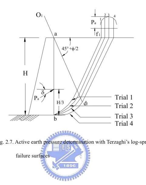
2.7 Active earth pressure determination with Terzaghi’s log-spiral surface ₆₀ 2.8 Comparison of coefficient of horizontal component of active pressure for

various theories (after Morgensern and Eisenstern, 1970) 61 2.9 MIT model retining wall (after Terzaghi, 1932) ₆₂ 2.10 Hydrostatic ratio as affected by yield of wall (after Terzaghi, 1934) ₆₃ 2.11 Height of center of pressure in relation to yield of wall (after Terzahi, 1934) 64 2.12 University of Manchester model retaining wall (after Mackey and Kirk,

1967) 65

2.13 Earth pressure with wall movement (after Mackey and Kirk, 1967) ₆₆ 2.14 Failure surface (after Mackey and Kirk, 1967) ₆₇ 2.15 College of Agriculture model retaining Wall (after Bros, 1972) ₆₈ 2.16 Active earth pressure coefficient with wall movement (after Bros, 1972) ₆₉ 2.17 Active earth pressure coefficient under both RT and RB mode with wall

movement 70

2.18 Shaking table, soil box, and actuator (after Sherif et al., 1982) ₇₁ 2.19 Shaking table with movable retaining wall (after Sherif et al., 1982) ₇₂ 2.20 Ksh, (h/H)s, and tan　 versus wall displacement S (after Sherif et al.,1982) ₇₃

Number Page 2.21 Experimental KSah values at S = H/1000 versus soil density (after Sherif et

al., 1982) 74

2.22 Change of normalized lateral pressure with wall rotation about top (loose backfill) (after Fang and Ishibashi, 1986) 75 2.23 Distribution of horizontal earth pressure at different wall rotation (rotation

about top) (after Fang and Ishibashi, 1986) 76 2.24 Distribution of horizontal earth pressure at different wall rotation (rotation

about base) (after Fang and Ishibashi, 1986) 77 2.25 Distribution of horizontal earth pressure Kh, relative height of resultant

pressure application h/H, and coefficient of wall friction tanδ, versus wall rotation (rotation about base) (after Fang and Ishibashi, 1986) 78 2.26 Change of normalized lateral pressure with translation wall

Displacement (after Fang and Ishibashi, 1986) 79 2.27 Distributions of horizontal earth pressure at different wall displacement

(rotation about base) 80

2.28 Coefficient of horizontal active thrust as a function of soil density (after

Fang and Ishibashi, 1986) 81

2.29 Schematic representation of retaining wall near rock face ₈₂ 2.30 Model retaining wall (after Frydman and Keissar, 1987) ₈₃ 2.31 Distribution of K’awith z/b from silo pressure equation(after Frydman and

Keissar, 1987) 84

2.32 (S/H)a versus backfill inclination (after Fang et al., 1997) ₈₅ 2.33 Active earth pressure coefficient Ka,h versus backfill inclination(after Fang

et al., 1997) 86

2.34 Finite element mesh (after Bakeer and Bhatia, 1989) ₈₇ 2.35 Effect of wall displacement on the earth pressure coefficient (K) (after

Bakeer and Bhatia, 1989) 88

2.36 Relative height resultant pressure (h/H)A as a function of 　 angle for

different modes of wall movement (after Matsuzawa and Hazarika,1996) 89 2.37 Horizontal active pressure coefficient KAcos 　as a function of 　 angle for

various modes of wall movement (after Matsuzawa and Hazarika, 1996) 90 2.38 Effect of wall displacement on location of the earth pressure resultant (Y/H)

(after Bakeer and Bhatia, 1989) 91

2.39 Typical space of backfill behind a retaining wall(after Fan and Chen, 2006) ₉₂ 2.40 Finite element mesh for a retaining wall with backfill(after Fan and Chen,

Number Page 2.41 Distribution of earth pressure at various wall displacements for T mode ₉₄ 2.42 Variation of KA as a function of β and d for walls T mode(after Fan and

Chen, 2006) 95

2.43 Influence of type of wall movement on coefficient of active earth pressures as a function of rock face inclination d = 0 (after Fan and Chen, 2006) 96 2.44 Influence of types of wall movement on the location of resultant of active

earth pressures for various inclinations of rock face at the backfill spacing d = 0 (after Fan and Chen, 2006)

97

3.1 NCTU model retaining wall ₉₈

3.2 Locations of pressure transducers on NCTU model wall ₉₉

3.3 Locations of driving rods ₁₀₀

3.4 Wall speed control system ₁₀₁

3.5 Data acquisition system ₁₀₂

3.6 Locations of driving rods ₁₀₃

3.7 Wall speed control system ₁₀₄

3.8 Data Acquisition System ₁₀₅

3.9 Picture of Data acquisition system ₁₀₆ 4.1 NCTU model retaining wall with inclined interface plate ₁₀₇

4.2 steel interface plate ₁₀₈

4.3 Steel interface plate ₁₀₉

4.4 Top-view of model wall ₁₁₀

4.5 NCTU model retaining wall with interface plate supports ₁₁₁ 4.6 Model retaining wall and steel interface plate ₁₁₂

4.7 Top supporting beam 113

4.8 Base supporting block 114

4.9 Base board 115

4.10 Model test with interface inclination β = 0° 116 4.11 Model test with interface inclination β = 50° 119 4.12 Model test with interface inclination β = 60° 121 4.13 Model test with interface inclination β = 70 123 4.14 Model test with interface inclination β = 80° 125

Number Page 5.1 Grain size distribution of Ottwa sand (after Hou, 2006) 127 5.2 Shear box of direct shear test device ₁₂₈ 5.3 Relationship between unit weight γ and internal friction angle φ (after

Chang, 2000) 129

5.4 Direct shear test arrangement to determinate wall friction ₁₃₀ 5.5 Relationship between unit weight γ and wall friction angle δ (after Lee, 1998) ₁₃₁

5.6 Lubrication layers on side walls ₁₃₂

5.7 Schematic diagram of sliding block test (after Fang et al., 2004) ₁₃₃ 5.8 Sliding block test apparatus (after Fang et al., 2004) ₁₃₄ 5.9 Variation of interface friction angle with normal stress(after Fang et al.,

2004) 135

510 Direct shear test arrangement to determine interface friction angle(after

Wang, 2000) 136

5.11 Relationship between unit weight γ and interface plate friction angle δi

(after Wang, 2005) 137

5.12 Relationship between unit weight γ and different friction angles ₁₃₈

5.13 Soil hopper ₁₃₉

5.14 Pluviation of the Ottawa sand into soil bin ₁₄₀ 5.15 Relationship between relative density of sand and drop height(after Ho,

1999) 141

5.16 Soil-density control cup ₁₄₂

5.17 Soil-density cup(after Chien, 2007) ₁₄₃ 5.18 Density control cups at the same elevation (top-view) ₁₄₄ 5.19 Density control cups at different elevation (side-view) ₁₄₅ 5.20 Distribution of relative density for loose sand ₁₄₆ 6.1 Model wall tests with different interface inclinations ₁₄₇ 6.2 Distribution of horizontal earth pressure for β = 0° ₁₄₈ 6.3 Variation of horizontal earth pressure versus wall movement for β = 0° ₁₄₉ 6.4 Relationship between σh/γz and S/H for β = 0° ₁₅₀ 6.5 Earth pressure coefficient Kh versus wall movement for β = 0° ₁₅₁ 6.6 Location of total thrust application for β = 0° ₁₅₂

Number Page 6.7 Distribution of horizontal earth pressure for β = 0° ₁₅₃ 6.8 Distribution of earth pressure for β = 60° ₁₅₄ 6.9 Variation of horizontal earth pressure versus wall movement for β = 50° ₁₅₅ 6.10 Relationship between σh/γz and S/H for β = 50° ₁₅₆ 6.11 Earth pressure coefficient Kh versus wall movement foe β = 50° ₁₅₇ 6.12 Location of total thrust application for β = 50° ₁₅₈ 6.13 Distribution of earth pressure for β = 50° ₁₅₉ 6.14 Distribution of earth pressure for β = 60° ₁₆₀ 6.15 Variation of horizontal earth pressure versus wall movement for β = 60° ₁₆₁ 6.16 Relationship between σh/γz and S/H at for β = 60° ₁₆₂ 6.17 Earth pressure coefficient Kh versus wall movement for β = 60° ₁₆₃ 6.18 Location of total thrust application forβ = 60° ₁₆₄ 6.19 Distribution of earth pressure for β = 60° ₁₆₅ 6.20 Distribution of earth pressure for 　 = 70° ₁₆₆ 6.21 Variation of the horizontal earth pressure versus wall movement for 　 =

70° 167

6.22 Relationship between 　h/　z and S/H for 　 = 70° ₁₆₈ 6.23 Earth pressure coefficient Kh versus wall movement for 　 = 70° ₁₆₉ 6.24 Location of total thrust application for 　 = 70° ₁₇₀ 6.25 Distribution of earth pressure for 　 = 70° ₁₇₁ 6.26 Distribution of earth pressure for 　 = 80° ₁₇₂ 6.27 Variation of horizontal earth pressure versus wall movement for 　 = 80° ₁₇₃ 6.28 Relationship between 　h/　z and S/H for 　 = 80° ₁₇₄ 6.29 Earth pressure coefficient Kh versus wall movement for 　 = 80° ₁₇₅ 6.30 Location of total thrust application for　 = 80° ₁₇₆ 6.31 Distribution of earth pressure for 　 = 80° ₁₇₇ 6.32 Variation of earth pressure coefficient K,h with increasing wall movement 178 6.33 Distribution of active earth pressure at different interface inclination angle

　 179

Number Page 6.35 Active earth pressure coefficient Ka,h versus interface inclination angle β 181 6.36 Point of application of active soil thrust versus interface inclination angle β 182 6.37 Normalized driving moment versus interface inclination angle β 183

List of Symbols

Cu = Uniformity Coefficient

d = Distance between Interface Plate and Model Wall Dr = Relative density

D10 = Diameter of Ottawa Sand whose Percent finer is 10% D60 = Diameter of Ottawa Sand whose Percent finer is 60% emax = Maximum Void Ratio of Soil

emin = Minimum Void Ratio of Soil

F = Force

Gs = Specific Gravity of Soil h = Location of Total Thrust

(h/H)a = Point of application of active soil thrust H = Effective Wall Height

i = Slop of Ground Surface behind Wall Ko = Coefficient of Earth Pressure At-Rest Ka = Coefficient of Active Earth Pressure Kh = Coefficient of Horizontal Earth Pressure

Ka,h = Coefficient of Horizontal Active Earth Pressure Pa = Total Active Force

RT = Rotation about Wall Top

RTT = Rotation about a Point above Wall Top RB = Rotation about Wall Base

RBT = Rotation about a Point below Wall Base β = Angle of inclination Rock Face

σh = Horizontal Earth Pressure σN = Normal Stress

S = Wall Displacement T = Translation

z = Depth from Surface γ = Unit Weight of Soil

φ = Angle of Internal Friction of Soil δi = Angle of Interface Friction δsw = Angle of Side-Wall Friction δw = Angle of Wall Friction τ = Shear Stress

Chapter 1

INTRODUCTION

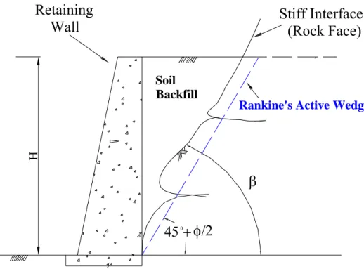
In this study, the effects of an adjacent inclined rock face on the active earth pressure against a rigid retaining wall is studied. In tradition, active earth pressure behind a gravity-type retaining wall is estimated with either Coulomb’s or Rankine’s theory. However, if the retaining wall is constructed on the side of for a mountainside highway, adjacent to an inclined rock face as shown in Fig. 1.1, the nearby rock face might intrude the active soil wedge behind the wall.. The distribution of earth pressure on the retaining wall might be affected by the presence of the inclined rock face. In the design of retaining walls in mountainous area, it is important to estimate the magnitude of the active soil thrust and the point of application of the active soil thrust.. For gravity-type retaining walls, the Rankine’s active failure wedge in the backfill is bounded by the wall and the plane with the inclination angle of (45° + φ/2) from the horizontal, as shown in Fig. 1.1 The nearby rock face may interfere the development of the Rankine’s active failure wedge behind the wall. For retaining walls built adjacent to stiff interface, can Coulomb’s or Rankine’s theory be used to evaluate the active earth pressure active on the wall? Would the distribution of active earth pressure still be linear with depth? The distribution of active earth pressure on retaining structures adjacent to an inclined stiff interface are discussed in this theis..

1.1 Objective of Study

The NCTU model retaining wall facility was modified to study the effects of an adjacent inclined rock face on active earth pressure. A steel interface plate simulating the rock face was designed contracted. A top supporting beam, and a base supporting

block was contracted to supporting steel interface plate. Air-dry Ottawa sand was used as backfill material. For a loose backfill, the soil was placed behind the wall with the air-pluviaiton method to achieve a relative density of 35%. The main parameter considered for this study is the rock face inclination angles β = 0°, 50°, 60°, 70° ,and 80° as in Fig.1.2. The height of the backfill H = 0.5 m. The variation of lateral earth pressure is measured with the soil pressure transducers on the surface of the model wall. Based on experimental results, the distribution of earth pressure on the retaining wall adjacent an inclined stiff interface are obtained. Base on the measurements obtained the instrumented NCTU model retaining wall, test results of this study would provide valuable information, for the geotechnical engineer to design retaining structures near a inclined rock face.

1.2 Research Outline

The subjects discussed in the thesis are summarized as follows. A review of theories and experimental findings associated with lateral earth pressures are summarized in Chapter 2. The Experimental apparatus for this study are discussed in Chapter 3. A steel interface plate was developed to simulate an inclined stiff interface. The details of the steel interface plate and its supporting system are discussed in Chapter 4. Chapter 5 introduces the properties of backfill and the distribution of density in the soil bin. The interface characteristics between the backfill and sidewall, model wall, and interface plate are also described in Chapter 5. Chapter 6 reports the experimental results regarding on earth pressure for interface. inclination angles β = 0o, 50o, 60o, 70o and 80o.

1.3 Organization of Thesis

This paper is divided into the following parts:

1. Introduction of the subject active earth pressure (Chapter 2) 2. Description of experimental apparatus (Chapter 3)

3. Description of interface plate and supporting system (Chapter 4) 4. Characteristics of the backfill and the interface (Chapter 5) 5. Experimental results for loose sand (Chapter 6)

Chapter 2

LITERATURE REVIEW

Geotechnical engineers frequently utilize the Coulomb and Rankine’s earth pressure theories to calculate the active earth pressure behind retaining structures. These theories will be discussed in the following sections. Terzaghi (1934), Mackey and Kirk (1967), Bros (1972), Sherif et al. (1982), Fang and Ishibashi (1986), Fang et al.(1994) and Fang et al.(1997) made experimental investigations regarding active earth pressure. Numerical investigation was studied by Bakeer and Bhatia (1989), Fang et al. (1993) and Matsuzawa and Hazarika (1996). Frydman and Keissar (1987) used the centrifuge technique to text a small mode. The change of pressure from the at-rest to the active condition for a retaining wall near a vertical rock face was observed. Fan and Chen (2006) used the non-linear finite element program PLAXIS to investigate the at-rest to the active condition for a rigid wall close to a stable rock face. Their major findings are introduced in this chapter.

2.1 Active Earth Pressure Theories

2.1.1 Coulomb Active Earth Pressure Theory

In 1776, Coulomb presented an analysis for determination of the active earth pressure against retaining walls. In Coulomb’s theory, the following assumptions are made.

1. Soil is isotropic and homogeneous.

2. The rupture surface is a plane surface, such as the plane BC shown in Fig. 2.1(a). The backfill surface is also a plane surface.

3. The frictional resistance is distributed uniformly along the rupture surface.

a a H K P 2 2 1_γ = 2 2 2 ) sin( ) sin( ) sin( ) sin( 1 ) sin( sin ) ( sin ⎭ ⎬ ⎫ ⎩ ⎨ ⎧ + − − + + − + = i i Ka β δ β φ δ φ δ β β β φ

developed between soil and wall. 5. Failure is a plane strain problem.

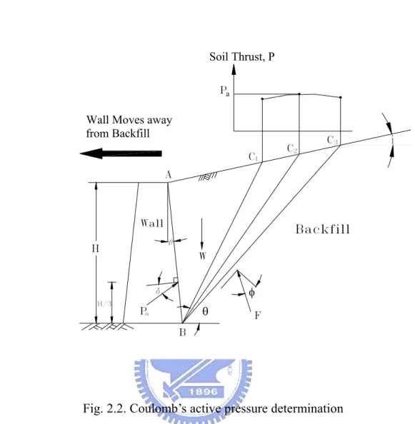
In order to develop an active state, the wall must move away from the soil mass. Then the wedge ABC moves down with respect to the wall and the wall friction angle δ develops at the soil-wall interface. The weight of wedge ABC is W and the force on BC is F. For a given value of θ, summation of forces in the vertical and horizontal directions allow us to calculate the resultant soil thrust P as shown in Fig. 2.1(b).

Similar force triangles for several trial wedges can be constructed, and the corresponding values of P can be determined. The illustration at the top of Fig. 2.2 shows the nature of variation of the P for different wedges. The maximum value of P is the Coulomb's active force Pa.

The summation of forces can be obtained analytically with the following equation ( (2.1) where

Pa = total active force per unit length of wall Ka = coefficient of active earth pressure γ = unit weight of soil

H = height of wall and

(. (2.2)

where

φ = internal friction angle of soil δ = wall friction angle

β = slope of back of the wall to horizontal i = slope of ground surface behind wall

a a γzK σ = a a H K P 2 2 1_γ = ) cos (cos cos ) cos (cos cos cos 2 2 2 2 φ φ − + − − = i i i i i Ka

2.1.2 Rankine Active Earth Pressure Theory

In 1875, Rankine considered the soil in a state of plastic equilibrium and used essentially the same assumptions as Coulomb. Except that Rankine assumed no friction between wall surface and backfill, and the backfill is cohesionless. The term plastic equilibrium in soil refers to the condition where every point in soil is on the verge of failure. The Rankine theory may be used if the earth pressure on the vertical plane AB is required; as illustrated in Fig. 2.3(a). In the figure it may be assumed that the earth pressure on plane AB is the same as that on plane AB inside a semi-infinite soil mass (Fig. 2.3(b)). For an active condition, at any given depth z, the active earth pressure σa can be expressed as:

( (2.3)

The total active force per unit length of the wall Pa is equal to

( (2.4)

The direction of resultant force Pa is parallel to the ground surface as shown in Fig. 2.3(b), where

( 2.5)

2.1.3 Terzaghi General Wedge Theory

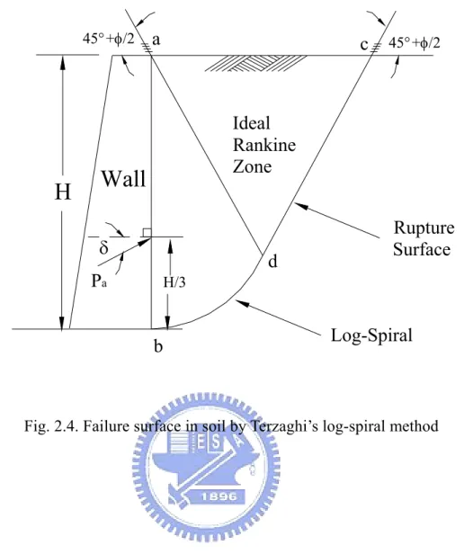
The assumptions made for Coulomb and Rankine theories are associated with plane failure surfaces. However, for a retaining structure with wall friction, the assumption does not apply in practice. Terzaghi (1941) suggested that the failure surface in the backfill under an active condition can be described with the log spiral curve bd, as shown in Fig. 2.4. It may be seen from the figure the failure surface dc is a plane surface.

φ θtan 0 1 r e r = ) 2 45 ( tan ) ( 2 1 2 2 1 1 φ γ °− = _d d H P

[ ]

2 1

[ ]

3 1

[ ]

1 1 l P l dF (0) P l W + _d + =

Fig. 2.5 illustrates the procedure to elevate the active resistance by trial wedge method (Terzaghi and Peck, 1967). The line d1c1 makes an angle of 45°+ φ/2 with the surface of the backfill. abd1c1 is a trial wedge in which bd1 is the arc of a logarithmic spiral described by the following equation

( (2.6) O1 is the center of the log spiral. (O1b = r1 and O1d1 = r0 and ∠bO1d1 = θ, refer to Fig. 2.5)

In consideration with the stability of the soil mass abd1f1 (Fig. 2.6), for equilibrium, the following forces per unit width of the wall are to be considered.

1. Weight of the soil in zone abd1f1 = W1 = γ ×(area of abd1f1)

2. The vertical face d1f1 is in the zone of Rankine’s active state; hence, the force Pd1 acting on the face is

( … (2.7)

where Hd1 = d1f1

Pd1 acts horizontally at a distance of Hd1/3 measured vertically upward form d1. 3. dF is the resultant of the shear and normal forces acting along the surface of

sliding bd1. At any point of the curve, according to the property of the logarithmic spiral, a radial line makes an angle φ with the normal. Since the resultant dF makes an angle φ with the normal to the spiral at its point of application, its line of application will coincide with a radial line and will pass through the point O1.

4. P1 is the active force per unit width of the wall. It acts at a distance of H/3 measured vertically form the bottom of the wall. The direction of the force P1 is inclined at an angle δ with the normal drawn to the back face of the wall. 5. Taking the moments of W1, Pd1, dF and P1 about the point O1, for

equilibrium

[

1 2 13

]

1 1 1 l P l W l P = + _d or (. (2.9)

where l₂, l3, and l1 are the moment arms for forces W1, Pd1, and P1, respectively.

The preceding procedure for finding the trial active force per unit width of the wall is repeated for several trial wedges as shown in Fig. 2.7. Let P1, P2, P3, …, Pn be the forces that correspond to trial wedges 1, 2, 3, …, n, respectively. The forces are plotted to the same scale as shown in the upper part of the figure. A smooth curve is plotted through the points 1, 2, 3, …, n. The maximum P1 of the smooth curve defines the active force Pa per unit width of the wall.

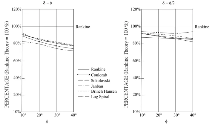
2.1.4 Comparison of K

a

for Various Theories

It is common to all the theories that the soil mass be in a state of limiting equilibrium, and shear strength of the soil be expressed in terms of the Mohr-Coulomb failure criterion. However, they differ in the assumption about the shape of the failure surface. For example, Coulomb theory (1776) assumes that sliding occurs along a planar sliding surface. The method developed by Brinch Hansen (1953) assumes the soil wedge slip along a circular surface. Janbu’s theory (1957) is not restricted to a particular shape of slip surface, but makes use of the method of slices and satisfied equilibrium in approximate manner. Terzaghi’s general wedge theory (1941) is based on logarithmic spiral slip surface.

The coefficient of active earth pressure Ka computed from various theories are compared by Morgenstern and Eisenstein (1970). Fig. 2.8 shows the variation of Ka as a function of internal friction angle φ of backfill, where the wall friction angleδis equal to φ and φ/2. For the case δ = φ/2, the total range of variation of Ka is generally less than 15% from Rankine’s solution. In this study, Ka values estimated with the Coulomb theory are compared with experiment results.

2.2 Laboratory Model Retaining Wall Tests

2.2.1 Model Study by Terzaghi

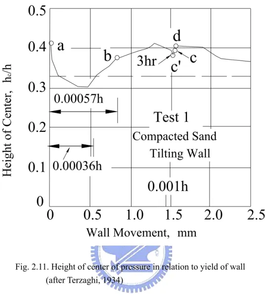
Terzaghi (1934) presented the test results on the lateral pressure of compacted sand against a large model wall. The face of the wall is 14 ft. long and 7 ft. high, while the internal dimension of the soil bin are 14 ft. ×14 ft. ×7 ft. (Fig. 2.9). Twenty Goldbeck pressure cell were used to measure the variation of earth pressure, ten built into the wall and ten rested into the floor of the bin. For a wall under translational sliding wall and Rotation about Base modes (RB) (Tilting wall), the earth pressure coefficient K (defined as σh/γz) measured at an elevation equal to one-half of the height of backfill is shown in Fig. 2.10. In this figure, only a very small wall displacement is required to reduce the earth pressure to values close to the fully active state. For a compacted backfill 4.5 ft. (1.372 m) high, an outward displacement of only about 1.5 mm (1/1000 of the depth of the backfill) would be needed to reach an active state. There is no difference between the K curves for a wall which yields by tilting (Test 1), and a wall which yields parallel to its original position (Test 2).

Fig. 2.11 shows the relation between the height of the center of pressure (defined as hc/h) and the yield of the wall. According to Coulomb’s theory, the center of pressure for level backfill should be located at one-third of the backfill depth above the base (hc/h= 0.33). For rotation about base modes (RB) (Tilting wall) mode, the height of center of pressure is lowered when the wall starts to move, but after wall movement equals to 0.00036h, the height of center of pressure gradual increased with increase wall movement.

2.2.2 Model Study by Mackey and Kirk

Mackey and Kirk (1967) described an experimental investigation into lateral earth pressure by using a steel model wall. This soil tank was made of steel with internal dimensions of 36 in. × 16 in. × 15 in. as shown in Fig. 2.12. In this investigation, when the wall moves away from the soil, the earth pressure decreases (see Fig. 2.13)

and then increases slightly until it reaches a constant value. Mackey and Kirk reported that if the backfill is loose, the active earth pressure obtained experimentally are within 14 percent off those obtained theoretically from almost any of the methods list in Table 2.1.

In the observation of the failure surface in the backfill, Mackey and Kirk utilized a powerful beam of light to trace the position of the shadow which formed by the change of level of the surface of the sand. It is found that the failure surface in the backfill due to the translational wall movement is approximated a curve (Fig. 2.14), instead of a plane as assumed by Coulomb.

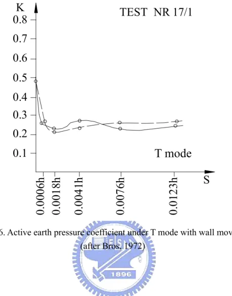
2.2.3 Model Study by Bros

Bros (1972) investigated the influence of different kinds of wall movement on the values and distribution of lateral active and passive pressures exerted against the model retaining wall. The model arrangement is illustrated in Fig. 2.15. The main structure consists of three vertical steel-frames supporting the soil bin which is 0.7m wide, 0.85 m high, and 1.6 m long. The pressure cells used are the diaphragm type. The earth pressures are measured with the deforming diaphragm with electric-resistivity strain gauges. In this study, clean, dry, quartz sand from Odra-river was used and the dense state was obtained by vibrating each 12-15 cm layer of sand with electric vibrator.

The outward translation of the wall caused the mobilization of friction between the backfill and side-wall, which tends to decrease the measured lateral pressures. The coefficient of horizontal earth pressure K as a function of wall displacement S is shown in Fig.2.16. It is concluded that, under a translational mode, the active condition was reached at the wall displacement of 0.0006h (h = height of backfill). As shown in Fig. 2.17 that, under both RB and RT mode, the active condition was reached at the wall displacement of 0.0035h and 0.0012h ~ 0.0018h, respectively.

2.2.4 Model Study by Sherif, Ishibashi, and Lee

dynamic earth pressure, and the test results were compared with the well-known Coulomb and Mononobe-Okabe equations. All of their experiments were conducted in the University of Washington shaking table and retaining wall assembly. The model system consists of four components: (1) shaking table and soil box; (2) loading and control units; (3) retaining wall; and (4) data acquisition system.

The shaking table is 3 m long, 2.4 m wide, and is made of steel as shown in Fig. 2.18(a). A rigid soil box 2.4 m long, 1.8 m wide, 1.2 m high is built on the shaking table for geotechnical earthquake engineering research. The movable model retaining wall and its driving system are shown in Fig. 2.19. The model wall consists of the main frame and the center wall. The center wall is 1 m wide, 1 m high, and 0.127 m thick. Six soil pressure transducers are mounted on the center line of the wall surface at different depths (Fig. 2.18b) to measure the soil pressure distribution against the main body of the center wall.

Fig. 2.20 shows the variation of Ksh, h/H and tanδ as a function of wall displacements, where δ is wall friction angle, (h/H) represent the point of application of the soil thrust, and Ksh is the static horizontal coefficient of earth pressure. The density of the loose Ottawa sand is ρ=1.54 g/cm3_{, and the corresponding φ angle is} 31.5o. The speed of wall movement was constant and equal to 1.5 x10-3 in/sec, and the patlern of wall movement was translational. It can be seen in Fig. 2.20 that the Kh values for loose soil reduce gradually until the wall is displaced significantly. It is reported that the Kh do not change significantly regardless of the soil density after the displacement H/1000. Sherif et al. reported that the experiment Ka,h shows good correlation with Coulomb’s expression, as shown in Fig. 2.21.

2.2.5 Model Study by Fang and Ishibashi

Fang and Ishibashi (1986) presented their experimental results regarding the distribution of the active stresses due to three different wall movement modes: (1) rotation about top; (2) rotation about heel; and (3) translation. Total active resultant forces and their points of application obtained from the experiments were

summarized. All experiments were conducted in the University of Washington shaking table and retaining wall facility.

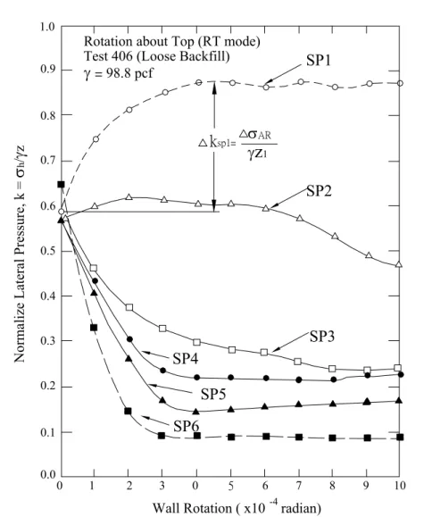
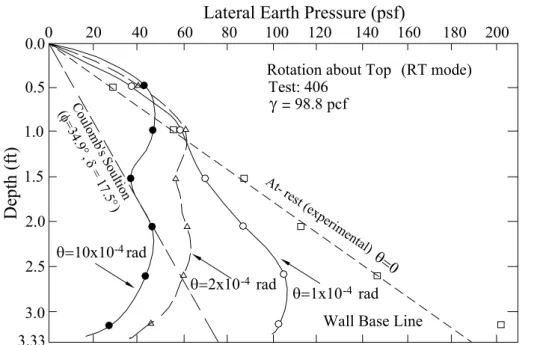
In Fig.2.22 it can be seen that the pressure behind the lower pressure transducer (SPT3, SPT4, SPT5 and SPT6) decreases quickly with wall rotation and then eventually nearly constant value. But the upper transducer (SPT1 and SPT2) increase initially with increasing wall rotation. In view of this, it is most probably due to arching formed in the upper portion of the backfill soil. Typical change of lateral stress distribution with different stages of wall rotation in Fig. 2.23. It can be seen the arching phenomenon dominates the backfill performance behind the upper portion of the wall when wall rotated about the top.

Fig. 2.24 shows a typical horizontal pressure distribution behind a wall rotated about the base. It is can be seen that lateral pressure of the upper elevation decrease very quickly, but the lateral pressure near the base of the wall decrease very slowly with wall rotation. The fully active state will be difficult to reach near the base. In view of this phenomenon, the horizontal earth pressure coefficient (Kh) drops rapidly

at the beginning and keeps the constant. Because of this, the total thrust will not be able to return to the H/3 position above the bottom of the wall (Fig. 2.25), which indicates the existence of the remaining part of the extra stress near the base of the wall.

Fig. 2.26 shows lateral earth pressures measured at various depths decreased rapidly with the translational wall displacement. Most measurements reach the minimum value at approximately 10 10_× −3

in (0.25 mm) wall displacement and stay steady thereafter.

The horizontal earth pressure distributions at different translational wall movements are shown in Fig. 2.27. The measured active stress is slightly higher than Coulomb's solution at the upper one-third of wall height, approximately in agreement with Coulomb's prediction in the middle one-third, and lower than Coulomb' at the lower one-third of wall surface. However, the magnitude of the active total thrust P_a

at S = 20 10× −3 in. (0.5 mm) is nearly the same as that calculated from Coulomb's theory. Fig. 2.28shows the Ka as a function of soil density and internal friction angle. In this figure, the Ka value decreases with increasing φ angle, and the Coulomb’s

solution would possible underestimate the coefficient Ka for rotational wall movement.

2.2.6 Frydman and Keissar’s Study

Frydman and Keissar (1987) used the centrifuge modeling technique to test a small model wall near a vertical rock face is shown in Fig. 2.29, and changes in pressure from the at-rest to the active condition was observed. The centrifuge system has a mean radius of 1.5 m, and can develop a maximum acceleration of 100 g, where g is acceleration due to gravity. The models are built in an aluminum box of inside dimensions 327 × 210 × 100 mm. Each model includes a retaining wall made from aluminum (195 mm high × 100 mm wide × 20 mm thick) as shown in Fig. 2.30. The rock face is modeled by a wooden block, which can, through a screw

arrangement, be positioned at varying distances b from the wall. Face of the block is coated with the sand used as fill, so that the friction between the rock and the fill is equal to the angle of internal friction of the fill

. Frydman and Keissar (1987) found that Spangler and Handy developed an equation, base on Janssen’s arching theory, for calculating the lateral pressure acting on the wall of the silo. The lateral pressure at any given depth, z, is given as (silo pressure equation).

σx = _⎥ ⎦ ⎤ ⎢ ⎣ ⎡ ⎟ ⎠ ⎞ ⎜ ⎝ ⎛− − δ δ γ tan 2 exp 1 tan 2 b z k b (2.10) where

σx= the lateral pressure acting on the wall

b = the distance between the wall

z = depth from wall top at which σx is required K = the coefficient of lateral earth pressure

γ = the unit weight of the backfill

δ = the angle of friction between the wall and the backfill

σv is the mean vertical pressure at given depth. The coefficient K value depends on the movement of the wall For walls without any movement, the Jaky’s equation was suggested for estimating the K value. In the active condition, Frydman and Keissar further derived the K value by taking into account the friction between the wall and the fill and assuming that the soil near the wall reached a state of failure .The K value is given by

(

₍

) (

)(

₎

)

1 sin tan 4 1 sin tan 4 sin 1 1 sin ) 1 (sin 2 2 2 2 2 2 2 2 + − + − − − + − + = φ δ φ δ φ φ φ K (2.11)

Where φ = the angle of internal friction of the fill. The coefficient of lateral earth pressure in the active condition at given depth z can be determined as the ratio of σx over σv(=γz), and is expressed as

_⎥ ⎦ ⎤ ⎢ ⎣ ⎡ ⎟ ⎠ ⎞ ⎜ ⎝ ⎛− − = δ δ γ tan 2 exp 1 tan 2 b z k z b b K_a (2.12)

The coefficient of active earth pressures at given depth z for a retaining wall near a vertical rock face can be theoretically estimated by substituting Eq. 2.11 into Eq. 2.12. The distribution of Ka value with the depth in Eq. 2.12 was verified using the experimental data obtained from the centrifuge model test, which the wall rotated about its base (RB model). The Ka value obtained decreased considerably with depth. Additionally, the measured Ka value was significantly less than the Rankine’s or Coulomb’s coefficient of active earth pressure. Fig. 2.31 shows the measured coefficient Ka value was in a range from 0.22 to 0.25 at z/b = 2, while it was about 0.14 at z/b = 6.5.

2.2.7 Model Study by Fang, Chang, and Chang

Fang et al. (1997) presented experimental data of earth pressure acting against a vertical rigid wall, which moved away from or toward a mass of dry sand with an inclined surface as shown in Fig 2.31. The instrumented NCTU retaining-wall facility was used to investigate the variation of earth pressure induced by the translational wall movement.

Based on their experimental data, it has been found that the earth-pressure distribution is essentially linear at each stage of wall movement. As shown in Fig. 2.32, the wall movement required for the loose backfill to reach an active stage increase with an increasing backfill inclination. Fig.2.33 shows the experimental active earth-pressure coefficients for various backfill sloping angles are in good agreement with the values calculated by Coulomb’s theory. It may be observed in the figure that it may not appropriate to adopt the Rankine theory to determine active earth pressure against a rigid wall with sloping backfill.

2.3 Numerical Study for Different Wall Movement

2.3.1 Numerical Study by Bakeer and Bhatia

Bakeer and Bhatia (1989) conducted finite element analyses to investigate the distribution of earth pressure for various wall movements. The finite element mesh consists of 247 two-dimensional quadrilateral isoperimetric eight-noded elements as shown in Fig. 2.34. The wall is represented by ten elements having the typical properties of concrete. In Fig. 2.35, the wall movement under RT mode (Rotation about Top), the coefficient of active earth pressure (K) is equal to 0.27, where the wall displacement reaches 0.0035 H. On the other hand, the minimum active earth coefficient of 0.4 is reached at the wall displacement of 0.003 H under RB mode (Rotation about Base). At any given displacement, the active earth coefficient for both RT and RB mode are higher than active earth coefficient for T mode.

Fig. 2.36 shows variation (Y/H) under different wall movement. In the figure, as the wall displacement increases, the point of application of the resultant force under the RT mode moved up to 0.55 H above the base of the wall, For RB mode, the earth pressure resultant moved increase with the wall displacement until it resultant acting at 0.215H above the base of the wall..

2.3.2 Numerical Study by Matsuzawa and Hazarika

Matsuzawa and Hazarika (1996) conducted numerical study to evaluate the effects of wall movement modes on active earth pressure. Interface elements with bi-linear stress-displacement relation were developed, and introduced between the soil and wall to simulate the interface frictional behavior. Conventional linkage elements were used to avoid separation between the wall and soil during the active movement of the wall. The active thrusts and point of application were found to be a function of the wall movement modes.

In Fig. 2.37(a) to (d), the coefficient of the horizontal active thrust coefficient KAcosδ are plotted against the angle of internal friction, for different modes of wall movements. For T mode, the analytical and experimental results for agreed closely with values given by Coulomb’s solution. However, for the RT mode (Fig 2.37(b)) and RB mode (Fig 2.37(c)) the numerical KAcosδ are higher than Coulomb value. However, under the RB-T mode (Fig 2.37(d)) the KAcosδ is lower than the Coulomb’s solution.

Fig. 2.38 shows the variation of the relative height of the point of application of the active thrust as a function of the backfill strength for the various wall movement modes. It can be seen from this figure expect that for the RB mode, both the analytical results and Dubrova’s solution agree well with the experimental data.

2.3.3 Numerical study by Fan and Chen

Fan and Chen (2006) used the non-linear finite element program PLAXIS to investigate the earth pressure from the at-rest to the active condition for a rigid wall

close to an inclined rock face. Fig. 2.39 the wall used for analysis is 5 m high, the back of the wall is vertical, and the surface of the backfill is horizontal. To investigate the influence of the adjacent rock face on the behavior of earth pressure, the inclination angle β of the rock face and the spacing d between the wall and the foot of the rock face were the parameters for numerical analysis. The wall was prevented from any movement during the placing of the fill. After the filling process active wall movement was allow until earth pressure behind walls reach the active condition. The wall was assumed to be rigid. Fig. 2.40 shows the finite element mesh, which has been examined to eliminate the influence of size effect and boundary effects. The finite element mesh consists of 1,512 elements, 3,580 nodes, and 4,536 stress points. Base on the numerical analysis, the distribution of earth pressure at various wall displacement for T mode is shown in Fig 2.41. The distribution of active earth pressure in active conditions with depth is non-linear. The calculated active pressure is considerably less than that computed using the Coulomb’s theory.

Fig. 2.42 shows the variation of the active earth pressure coefficient k computed with finite element analysis, as a function of the inclination of the rock face and rock face-wall spacing d, for walls under T mode. The analytical active K values are consider than less than those calculated with Coulomb’s solution. The analytical K value decrease and decrease with decreasing β angle, for β angle less than5 30°. Fig. 2.43 shows the variation of the KA with the β angle at d = 0 with T, RT and RB mode.

Fig. 2.44 shows the variation of the point of application of the active soil thrust with the β angle for d = 0. The variation of the h/H value with the β for walls in RB and T modes are similar. For walls in RB and T modes, the h/H decrease with increasing β angles, then it levels off h/H=0.333 for β angles greater than about 30°. However, the analytical h/H values were much higher than those for RB and T modes.

Chapter 3

EXPERIMENTAL APPARATUS

In order to study the earth pressure behind retaining structures, the National Chiao Tung University (NCTU) has built a model retaining wall system which can simulate different kinds of wall movement. All of the investigations described in the thesis were conducted in this model wall, which will be carefully discussed in this chapter. The entire system consists of the following components: (1) soil bin; (2) model retaining wall; (3) driving system; and (4) data acquisition system. The arrangement of the NCTU model retaining wall system is shown in Fig.3.1 and Fig. 3.2.

3.1 Soil Bin

The soil bin is 2,000 mm in length, 1,000 mm in width and 1,000 mm in depth as shown in Fig. 3.1. Both side walls of the soil bin are made of 30 mm thick transparent acrylic plates, through which the behavior of the backfill can be observed. Outside the acrylic plates, steel beams and columns are used to confine the side walls to ensure a plane strain condition.

The end wall that sits opposite to the model retaining wall is made of 100 mm thick steel plates. All corners, edges and screw-holes in the soil bin have been carefully sealed to prevent soil leakage. The bottom of the soil bin is covered with a layer of Safety-Walk to provide adequate friction between the soil and the base of the soil bin. The bed located below the retaining wall is fixed and serves to hold the bottom 113 mm of backfill, in order to accommodate a log spiral failure surface under passive condition. For this study, only active earth pressure experiment were conducted. The space in the soil bin below the model wall was filled with the base supporting block and base Supporting Boards as discussed in section 4.2.2. The 337 mm high dead load on top of the movable wall is designed to resist the uplift component of passive earth pressure that might act on the wall.

that the lateral deformations of the side walls will be negligible. The friction between the backfill and the side walls is to be minimized to nearly frictionless, so that shear stress induced on the side walls will be negligible. To eliminate the friction between backfill and sidewall, a lubrication layer with 3 layers of plastic sheets was furnished for all model wall experiments. The “thick” plastic sheet was 0.152 mm thick, and it is commonly used for construction, landscaping, and concrete curing. The “thin” plastic sheet was 0.009 mm thick, and it is widely used for protection during painting, and therefore it is sometimes called painter’s plastic. Both plastic sheets are readily available and neither is very expensive. The lubrication layer consists of one thick and two thin plastic sheets were hung vertically on each sidewall of the soil bin before the backfill was deposited. The thick sheet was placed next to the soil particles. It is expected that the thick sheet would help to smooth out the rough interface as a result of plastic-sheet penetration under normal stress. Two thin sheets were placed next to the steel sidewall to provide possible sliding planes. Tests to study the lubrication effects of the plastic sheets will be discussed in section 5.3..

3.2 Model Retaining Wall

The moveable retaining wall and its driving systems are shown in Fig. 3.1. The retaining wall is 1000 mm wide, 550 mm high, and 120 mm thick, and is made of solid steel. The retaining wall is vertically supported by two unidirectional rollers , and lateral supported by the steel frame through the driving system. Two separately controlled wall driving mechanism, one at the upper level, and the other at the lower level, provide various kinds of lateral wall movements.

Each wall driving system is powered by variable-speed motor. The motors turn the worm driving rods which cause the driving rods to move the wall back and forth. Two displacement transducers (Kyowa DT-20D) are installed at the back of retaining wall and their sensors are attached to the movable wall. Such an arrangement of displacement transducers would be effective in describing the wall translation and rotation. Table 3.1 shows the range of wall displacement reported by previous researchers for different wall movement modes to achieve an active state of stress.

Based on their studies, the wall displacements from 0.0005H to 0.0040H could lead to active states.

To investigate the earth pressure distribution, 9 earth pressure transducers (PGM-02KG, capacity = 19.62kN/m2) were attached to the model wall. The arrangement of the earth pressure cells should be able to closely monitor the variation of the earth pressure of the wall with depth. Base on this reason, the earth pressure transducers SPT1 through SPT9 have been arranged at two vertical columns as shown in Fig. 3.3 and Fig. 3.4.

A total of 9 earth pressure transducers have been arranged within a narrow central zone to avoid the friction that might exist near the side walls of the soil bin as shown in Fig. 3.3. The soil pressure transducers are strain-gage-type transducers (PGM-02KG, capacity = 19.62kN/m2) as shown in Fig. 3.5. To eliminate the soil arching effect, all soil pressure transducers are built quite stiff, and their measuring surfaces are flush with the face of the wall. They provide closely spaced data points for determining variation of the earth pressure distribution with depth.

3.3 Driving System

To achieve different modes of wall movement, two sets of driving rods are attached to the model wall. The upper driving rods are located 230 mm below the top of the wall, and the lower rods are located 236 mm below the upper rods as shown in Fig. 3.6. Two driving motors (ELECTRO, M-4621AB) supply the thrust to the upper and the lower driving rods independently. The wall speed and movement modes are controlled by the automatic motor speed control system (DIGILOK, DLC-300) shown in Fig. 3.7. By setting the same motor speed for the upper and lower driving rods, a translation mode can be achieved for the model wall.

3.4 Data Acquisition System

transducers and displacement transducers, a data acquisition system shown in Fig. 3.8 was used for this study. It is composed of the following four parts: (1) dynamic strain amplifiers (Kyowa: DPM601A and DPM711B); (2) NI adaptor card; (3) AD/DA card; and (4) personal computeras shown in Fig. 3.9. The analog obtained signals from the sensors are filtered and amplified by dynamic strain amplifiers. Analog experimental data are converted to digital data by the A/D – D/A card. The LabVIEW program is used to acquire test data. Experimental data are stored and analyzed with a Pentium 4 personal computer.

Chapter 4

Interface Plate and Supporting System

A steel interface plate is designed and constructed to simulate inclined rock face near the retaining structure shown in Fig. 1.1. In Fig. 4.1, the plate and its supporting system are developed to fit in the NCTU model retaining-wall facility. The interface plate consists of two parts: (1) steel plate; and (2) reinforcing steel beams. The supporting system consists of the following three parts: (1) top supporting beam; (2) base supporting block; and (3) base supporting board. Details of the interface plate and its supporting system are introduced in the following sections.

4.1 Interface Plate

4.1.1 Steel Plate

The steel plate is 1.370 m-long, 0.998 m-wide, and 5 mm-thick as shown in Fig. 4.2. The unit weight of the steel plate is 76.52 kN/m3 and its total mass is 53.32 kg (0.523 kN). A layer of anti-slip material (Safety-walk, 3M) is attached on the steel plate to simulate the friction that acts between the backfill and rock face as illustrated in Fig. 4.2 (c) and Fig. 4.3 (a). For the inclination angle β = 50o _{shown in Fig. 1.2, the} length of the interface plate should be at least 1.370 m. On the other hand, the inside width of the soil bin of the NCTU retaining wall facility is 1 m. In order to put the interface plate into the soil bin, the width of the steel plate has to less than 1.0 m. As a result, the steel plate was designed to be 1.370 m-long and 0.998 m-wide.

4.1.2 Reinforcement with Steel Beams

To simulate the stiffness of the rock face shown in Fig. 1.1, the steel interface plate should be nearly rigid. To increase the rigidity of the 5 mm-thick steel plate, Fig. 4.2 (b) and Fig. 4.3 (b) shows 5 longitudinal and 5 transverse steel L-beams directions were welded to the back of steel plate. Section of the steel L-beam (30 mm × 30 mm × 3 mm) was chosen as the reinforced material. On top of the interface plate, a 65 mm × 65 mm × 8 mm steel L-beam was welded to reinforce the connection between the plate and the hoist ring shown in Fig. 4.3 (b).

4.2 Supporting System

To keep the steel interface plate in the soil bin stable during testing, a new supporting system for the interface plate was designed and constructed. A top-view of the base supporting frame is illustrated in Fig. 4.4. The supporting system composed of the following three parts: (1) base block; (2) top supporting beam; (3) base boards as shown in Fig. 4.5 and Fig. 4.6. these parts are discussed in following sections.

4.2.1 Top Supporting Beam

In Fig. 4.5, the top supporting steel beam is placed at the back of the interface plate and fixed at the bolt slot of the side wall of the soil bin. Details of top supporting beam are illustrated in Fig. 4.7. The section of supporting steel beam is 65 mm × 65 mm × 8 mm and its length is 1700 mm. Fig. 4.4 shows four bolt slots were drilled on each side of the U-shape steel beam on the side wall of the soil bin. Fig. 4.6 (b) shows the top supporting beam was fixed at the slots with bolts.

4.2.2 Base Supporting Block and Base Board

The base block used to support the steel interface plate is shown in Fig. 4.8. The supporting block is 1 m-long, 0.14 m-wide, and 0.113 m-thick. Fig. 4.8 (b) shows

an three trapezoid grooves were caved to the face of the base supporting block. Fig. 4.5 shows the foot of the interface plate could be inserted into the groove at different distance from the model wall. Different horizontal spacing d adopted for testing includes: (1) d = 0 mm (2) d = 50 mm and (3) d = 100 mm. Fig. 4.5 shows 6 base boards are placed between the base supporting block and the end wall to keep the base block stable. Details of base boards are illustrated in Fig. 4.9. The base board is 1860 mm-long, 1002 mm-wide and 113 mm-thick. The surface of the top base board was cover with a layer of anti-slip material Safe-Walk.

4.3 Different Interface Inclinations

Different interface inclinations angles β = 0o_{, 50}o_{, 60}o_{, 70}o _{and 80}o _associated with this investigation are shown in Fig. 4.10 to Fig. 4.14. Fig. 4.10 (a) shows the test condition for inclination angle β = 0o_{. Fig.4.10 (b) shows Ottawa sand was pluviated} into the soil bin without the interface plate, Fig. 4.10 to Fig. 4.13 show the arrangement of model wall, plastic sheets interface plate and Ottawa sand conditions for the interface inclination angle β = 50o_{, 60}o_{, 70}o _{and 80}o_.

Chapter 5

BACKFILL AND INTERFACE

CHARACTISTICS

This chapter introduces the properties of the backfill, and the interface characteristics between the backfill and the wall. Laboratory experiments have been conducted to investigate the following subjects: (1) backfill properties; (2) interface characteristics between model wall and backfill; (3) side wall friction; (4) interface plate friction; and (5) distribution of soil density in the soil bin. The parameter of loose sand used for this study are summarized in Table 5.1

5.1 Backfill Properties

Air-dry Ottawa silica sand (ASTM C-778) was used as backfill. Physical properties of Ottawa sand are listed in Table 5.2 Grain-size distribution of the backfill is shown in Fig. 5.1. Major factors considered in choosing Ottawa sand as the backfill material are summarized as follows.

1. Its round shape, which avoids effect of angularity of soil grains.

2. Its uniform distribution of grain size (coefficient of uniformity Cu=1.78), which avoids the effects due to soil gradation.

3. High rigidity of solid grains, which reduces possible disintegration of soil particles under loading.

4. Its high permeability, which allows fast drainage of pore water and therefore reduces water pressure behind the wall.

To establish the relationship between unit weight γ of backfill and its internal friction angle φ, direct shear tests have been conducted. The shear box used has a square (60 mm×60 mm) cross-section, and its arrangement are shown in Fig. 5.2.

Chang (2000) established the relationship between the internal friction angle φ and unit weight γ of the ASTM C-778 Ottawa sand as shown in Fig. 4.3. It is obvious from the figure that soil strength increases with increasing soil density. For the air-pluviated backfill, the empirical relationship between soil unit weight γ and φ angle can be formulated as follows

φ

= 6.43γ - 68.99 (5.1) where

φ

=angle of internal friction of soil (degree) γ =unit weight of backfill (kN/m3)

Eqn. (5.1) is applicable for γ= 15.45 ~ 17.4 kN/m3 only.

5.2 Interface Characteristics between Model Wall and

Backfill

To evaluate the wall friction angle δw between the backfill and model wall, special direct shear tests have been conducted. A 88 mm × 88 mm × 25 mm smooth steel plate, made of the same material as the model wall, was used as the lower shear box. Ottawa sand was placed into the upper shear box and vertical load was applied on the soil specimen. The arrangement of this test is shown in Fig. 5.4.

To establish the wall friction angles developed between the steel plate and sand, soil specimens with different unit weight were tested. Air-pluviation methods was used to achieve different soil density, and the test result is shown in Fig. 5.5. For air-pluviation Ottawa sand, Lee (1998) suggested the following relationship:

δw= 2.33γ - 17.8 (5.2)

Eqn. (5.2) is applicable for γ = 15.5~17.5 kN/m3 _{only. The φ angle and δ angle} obtained in section 5.1 and 5.2 are used for calculation of active earth pressure for

5.3 Side Wall Friction

To constitute a plane strain condition for model wall experiments, the shear stress between the backfill and sidewall should be eliminated. A lubrication layer fabricated with plastic sheets was equipped for all experiments to reduce the interface friction between the sidewall and the backfill. The lubrication layer consists of one thick and two thin plastic sheets as suggested by Fang et al.(2004). All plastic sheets had been vertically placed next to both side-walls before the backfill was deposited as shown in Fig. 5.6.

The friction angle between the plastic sheets and the sidewall was determined by the sliding block tests. The schematic diagram and the photograph of the sliding block test by Fang et al. (2004) are illustrated in Fig. 5.7 and Fig. 5.8. The sidewall friction angle δ_sw is determined based on basic physics principles. Fig. 5.9 shows the variation of interface friction angle δ_sw with normal stress σ based on the plastic sheet lubrication method. The friction angle measured was 7.5°. With the plastic – sheet lubrication method, the interface friction angle is almost independent of the applied normal stress. The shear stress between the acrylic side-wall and backfill could be effectively reduced with the plastic-sheet lubrication layer.

5.4 Interface Plate Friction

To evaluate the interface friction between the interface plate and the backfill special, direct shear tests were conducted as shown in Fig. 5.10. In Fig. 5.10(b),a 80 mm × 80 mm × 15 mm steel plate was covered with a layer of anti-slip material “Safety-Walk” to simulate the surface the interface plate.Theinterface plate was used to simulate the inclined rock face show in Fig. 1.1. Ottawa sand was placed into the upper shear box and vertical stress was applied on the soil specimen as shown in Fig. 5.10(a).

To establish the relationship between the unit weight γ of the backfill and the interface-plate friction angleδi, soil specimens with different unit weight were tested.

Air-pluviation methods was used to achieve different soil density, and the test result is shown in Fig. 5.11. For air-pluviation Ottawa sand, Wang (2005) suggested the following empirical relationship:

δ i = 2.7γ- 21.39 (5.3) where

δi = interface-plate friction angle (degree) γ = unit weight of backfill (kN/m3₎

Eqn. (5.3) is applicable for γ = 15.1 ~16.36 kN/m3 _only.

The relationships between backfill unit weight γ and different friction angles are illustrated in Fig. 5.12. The internal friction angle of Ottawa sand φ, model wall-soil friction angleδw, interface-plate friction angleδi, and sidewall friction angle δsw as a function of δ are compared in the figure. It is clear in Fig. 5.12 that, with the same unit weight, the order of 4 different friction angles is φ ＞δi ＞δ w ＞δsw.

5.5 Control of Soil Density

5.5.1 Air-Pluviation of Backfill

To achieve a uniform soil density in the backfill, dry Ottawa sand was deposited by air-pluviation method into the soil bin. The air-pluviation method had been widely used for a long period of time to reconstitute laboratory sand specimens. Rad and Tumay (1987) reported that pluviation is the method that provides reasonably homogeneous specimens with desired relative density. Lo Presti et al. (1992) reported that the pluviation method could be performed for greater specimens in less time. As indicated in Fig. 5.13, the soil hopper that lets the sand pass through a calibrated slot opening at the lower end was used for the spreading of sand. A picture showing air-pluviation of the Ottawa sand into soil bin is indicated in Fig. 5.14. Air-dry Ottawa sand was shoveled from the soil storage bin to the sand hopper, weighted on the