利用位能場模型作路徑規劃及物體形狀比對

(1)

國立交通大學

資訊科學研究所

博士論文

利用位能場模型作路徑規劃及物體形狀比對

Potential-Based Path Planning and Shape

Matching

研究生：林建州

指導教授：莊仁輝博士

(2)

利用位能場模型作路徑規劃及物體形狀比對

Potential-Based Path Planning and Shape Matching

研

究

生：林建州 Student：Chien-Chou Lin

指導教授：莊仁輝

Advisor：Jen-Hui Chuang

國立交通大學

電機資訊學院

資訊科學研究所

博士論文

A Thesis

Submitted to Institute of Computer and Information Science

College of Electrical Engineering and Computer Science

National Chiao Tung University

in Partial Fulfillment of the Requirements

for the Degree of Doctor of Philosophy

in

Computer and Information Science

September 2004

Hsinchu, Taiwan, Republic of China

(3)

利用位能場模型作路徑規劃及物體形狀比對

研究生：林建州

指導教授：莊仁輝博士

國立交通大學資訊科學研究所

摘要

本博士論文乃利用位能場模型來呈現自由空間的方法，探討位能場於不同問題的應用。我們提出數個以位能場模型為基礎的演算法來協助解決（1）機器人路徑規劃與（2）物體形狀比對的問題。在這些演算法中，其共同的主要概念是將物體及自由空間的邊界帶相同之電性後，靜止的自由空間會有位能場形成，且自由空間對物體產生推斥力，再將作用於物體上的推斥力作為物體移動的推力與轉動的轉矩，使物體降低在自由空間中位能與自由空間達成最佳的形狀比對，物體的形式可以是剛體或是連結物。最佳的形狀比對可藉由調整物體的位置、姿態來降低位能而達成。在機械手臂路徑規劃研究中，我們探討了利用牛頓位能場應用於二維路徑規劃問題的可行性。在研究中，我們將機械手臂及自由空間的邊界以均勻或不均勻的帶電後，如同於電學中的定義，可計算得知機械手臂在工作空間中所受的斥力與轉矩，藉由這些斥力與轉矩來調整手臂於自由空間之組態使其位能降低。透過尋找這一連串的組態後，一條避碰的路徑即可由這些一系列組態來構成。我們也將上述演算法推廣到三維工作空間，亦即將原來牛頓位能場模型用三維廣義位能場 [1] 來取代。在 [1] 中提到，牛頓位能場模型在三維空間之中會造成物體撞入障礙物中，並不能達到避碰的要求。因而，我們採用廣義位能場模型來達成避碰。相對於機械手臂的基點是固定的，連結型機器人因有可移動的基點所以在路經規劃上有較高的自由度。在本論文中，我們亦發展了相對應之路徑規劃演算法。另外，透過相同的廣義位能場模型的建立，我們亦提出一三維物體形狀比對的演算法。在 [2] 中，廣義位能場模型被用來做單一剛體在一靜態空間的路徑規劃；

(4)

事實上，在路徑規劃的過程中，降低剛體於靜態空間位能的作法可視為某種程度的剛體與自由空間的形狀比對。在路徑規劃演算法中，剛體位置會沿著路徑改變、但大小不變；然而，在形狀比對中，比對物體的位置變化不大，但其大小卻會隨之增長。當比對物體增大後，如能調整其位置及姿態以降低位能，則可獲得一個較好的比對形狀。此外，由於三維物體資料經常為點資訊（如 range data），資料量大且不易解讀，以位能場為基礎之形狀比對演算法可直接使用物體的點資訊作比對，可省去費時的物體點資訊前處理。由實驗結果得知，所提出的演算法在物體之路徑規劃與形狀比對均有不錯之成果，而後者對於部分遮蔽的物體亦可適用。關鍵字：廣義位能場，路徑規劃，障礙物避碰，形狀比對

(5)

Potential-Based Path Planning and Shape Matching

Student：Chien-Chou Lin

Advisor：Dr. Jen-Hui Chuang

Institute of Information and Computer Science

National Chiao Tung University

Abstract

In this thesis, along the general direction of free space modeling using potential models, various applications of potential models are investigated. Variant potential-based algorithms are proposed to solve (1) path planning and (2) shape matching problems. The common idea of these algorithms is to use the repulsion exerted on an object, in forms of repulsive force and torque, from free space boundaries to achieve the best shape match between them. The object can be rigid or articulated, and the best match in shape is accomplished by adjusting object configuration, i.e., location and orientation, to minimize the potential fields among them.

In the path planning algorithm of manipulators, the Newtonian potential is used to represent manipulators and obstacles with charged boundaries in a 2-D workspace. The approach computes, similar to that done in electrostatics, repulsive force and torque between charged objects in the workspace. A collision-free path of a manipulator will then be obtained by locally adjusting the manipulator configuration to search for minimum potential configurations using these force and torque. The proposed approach is efficient because these potential gradients are analytically tractable. The above potential-based path planning approach for manipulators is extended to three dimensions using the generalized potential model [1] instead of Newtonian potential. In [1], it is shown that the Newtonian potential, being harmonic in the 3-D space, can not prevent a charged point object from running into another object whose surface is uniformly charged. While the base of a manipulator is fixed, an articulated robot has higher DOF due to its moving base. A modified path planning algorithm based on the same generalized potential model is also proposed for articulated robots with moving bases in this thesis.

(6)

potential-based path planner for a single rigid robot among stationary and rigid obstacles in 3-D workspace. Indeed, the minimization of potential between robots and obstacles is a shape matching procedure of a robot within a free space in some respects. While a rigid robot moves along a path in a free space without changing its size in path planning, the object stays about the same location inside the shape template with growing size in shape matching. According to the proposed approach, a better match in shape between the template object and the input object can be obtained if the input object translates and reorients itself to reduce the potential while growing in size. Since objects are usually represented by mass and unstructured row data, e.g., range data, existed shape matching algorithms may have a preprocessing procedure to extract features from row data of objects. However, the proposed potential-based algorithm can directly perform the matching with range data of objects without preprocessing procedures. Simulation results show that the proposed algorithms work well for both path planning and shape matching applications. The latter is also practicable to objects with incomplete surface descriptions, e.g., due to a partial view.

Keywords: generalized potential model, path planning, obstacle avoidance, shape

(7)

List of Figures

2.1 Coordinate transformation. (a) The original coordinate system (xy-plane).

(b) The new coordinate system (uv-plane) after the transformation. . . . 7

2.2 A polygonal surface S in the 3-D space. . . . 11

2.3 Geometric quantities associated with a point, an edge Ci (subscript i is omit-ted) of S shown in Figure 2.2 and the plane Q containing S. . . . 12

2.4 The sampling model for a link of a manipulator. . . 14

3.1 A manipulator is moved toward the goal (not shown) by sequentially traversing a sequence of GLs. . . 16

3.2 Basic planning procedure for a given GL. . . 17

3.3 Sliding p along ellipse E1, by translating lnkn to reduce the repulsive potential. 20 3.4 A path planning example derived from [54]. . . 22

3.5 A path planning example derived from [55]. . . 22

3.6 A various δ example derived from [5]. . . . 23

3.7 A 9-link manipulator example. . . 24

4.1 A manipulator is moved toward the goal (not shown) by sequentially traversing a sequence of GPs. . . 26

4.2 The generalized cylinder presentation of a passage. . . 26

4.3 Basic path planning procedure for a given GP (see text). . . 28

4.4 Sliding p on GP10, by translating lnk_n to reduce the repulsive potential. . . . 32

4.5 A path planning example for a 6-link manipulator in a 3-GP workspace. (a) The initial configuration. (b) The final configuration. . . 33

4.6 Side views of the initial configuration of manipulator, as well as intermediate configurations as its end-effector reaches each of the three GPs in Fig. 4.5. . 34

(11)

4.7 (a) The complete manipulator trajectory. (b) The partial trajectory between Figs. 4.6(a) and (b). (c) The partial trajectory between Figs. 4.6(b) and (c). (d) The partial trajectory between Figs. 4.6(c) and (d). . . 34 4.8 A path planning example for a 6-link manipulator in a 4-GP workspace. (a)

The initial configuration. (b)-(c) Two different views of the final configuration. 35 4.9 Top views of the initial configuration of the manipulator, as well as

interme-diate configurations as its end-effector reaches each of the four GPs in Fig. 4.8. . . 36 4.10 (a) The complete manipulator trajectory. (b) The partial trajectory between

Figs. 4.9(a) and (b). (c) The partial trajectory between Figs. 4.9(b) and (c). (d) The partial trajectory between Figs. 4.9(c) and (d). (e) The partial trajectory between Figs. 4.9(d) and (e). . . 36 4.11 A path planning example for a 6-link manipulator in a 3-GP blocked workspace.

(a)-(b) Two different views of the initial configuration. (c) The final configu-ration. . . 37 4.12 Side views of the intermediate configurations as its end-effector reaches each

of the three GPs in Fig. 4.11. . . 37 4.13 Manipulator configurations shown in Fig. 4.12 observed from a different

view-ing angle. . . 38 4.14 (a) The partial trajectory between Figs. 4.11(a) and 4.12(a). (b) The partial

trajectory between Figs. 4.12(a) and (b). (c) The partial trajectory between Figs. 4.12(b) and (c). . . 38 4.15 Partial manipulator trajectories shown in Fig. 4.14 observed from a different

viewing angle. . . 39

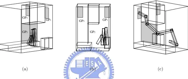
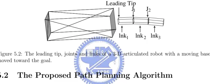
5.1 A 3-D articulated robot is to move toward the goal by sequentially traversing a sequence of GPs. . . 41 5.2 The leading tip, joints and links of a 3-D articulated robot with a moving

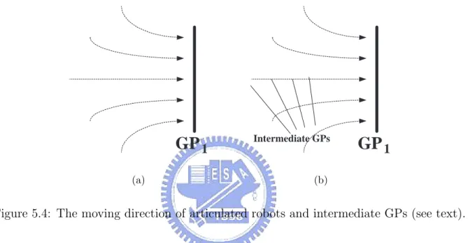
base moved toward the goal. . . 41 5.3 Basic path planning procedure for a given GP (see text). . . 43 5.4 The moving direction of articulated robots and intermediate GPs (see text). 43 5.5 Translating lnk1 to slide p on GP10 to reduce the repulsive potential. . . 46

(12)

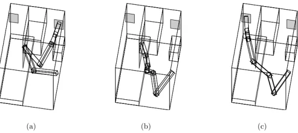
5.6 A path planning example for a 3-link articulated robot in a 3-GP workspace. (a) The initial configuration. (b) The trajectory. . . 48 5.7 A path planning example for a 3-link articulated robot in a 2-GP workspace.

(a) The initial configuration. (b) The final trajectory.(c) The 248-triangle tunnel. . . 49 5.8 A path planning example for a 4-link articulated robot in a 4-GP passage. (a)

The initial configuration. (b) The final trajectory. . . 50 5.9 A path planning example for a 4-link articulated robot in a 5-GP workspace.

(a) The initial configuration. (b) The final trajectory. . . 51 5.10 A path planning example like Fig. 5.7 with 248 triangles of obstacles. . . 51 5.11 The computation time will be proportional to the number of triangles of

ob-stacles, and the number of robot configurations calculated. (a) Computation time vs. Number of triangles of obstacles. (b)Computation time vs. Number of links. . . 52 5.12 Path planning examples for a 4-link articulated robot in an U-shaped workspace

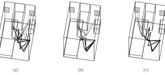
with (a) 3 (b) 4 and (c) 5 initial GPs. . . 53 5.13 Successful paths of Figs. 5.12(b)(c), respectively. . . 54 5.14 A path planning example for a 3-link articulated robot in a 3-GP workspace.

(a) The initial configuration. (b) The trajectory. . . 54 5.15 Since Ti−1 is perpendicular with T i, the lnki should rotate with respect to Si

to let T0

i moves to Ti. . . 55

5.16 Two planned paths for a 3-link articulated robots with 2-DOF and 3-DOF Joints. (a) The third configuration of the robot with 2-DOF joints. (b) The third configuration of the robot with 3-DOF joints. . . 55 5.17 Two planned paths for a 3-link articulated robots with 2-DOF and 3-DOF

Joints in the same environment.(a) A 24-configuration path of the robot with 2-DOF joints. (b) A 24-configuration path of the robot with 3-DOF joints. . 56

6.1 The basic shape matching procedure: (a) place a (size-reduced) input object inside a template object, (b) translate and (c) rotate the input object to reduce the potential, then (d) increase the size of the input object. . . 58

(13)

6.2 With its centroid chosen as the rotation center, the inner rectangular will experience local minima in the potential value at four angular positions. . . . 61 6.3 The arbitrarily chosen object axis is passing through the object centroid and

is parallel to the z-axis. . . . 61 6.4 Four directions of object axis used to generate twelve initial object orientations. 62 6.5 Images of some object models. . . 63 6.6 Shape matching results obtained for four input objects. . . 65 6.7 Shape matching results for propane (left) and piston (right). . . . 65 6.8 The CPU time spent in the shape matching for propane as a function of the

amount of input data. . . 66 6.9 Matching results using partial views of, from top to bottom, dean, dodecahdrn,

M − 104, M − 110, and M − 112. . . . 67 6.10 Matching results using partial views of propane and piston. . . . 68 6.11 Matching results with (a) 5% and (b) 10% noise contamination in the input

data. . . 69 6.12 (a) An unsuccessful shape matching result due to a highly uneven distribution

of input data. (b) The result obtained by using a subset of the input data. . 69 6.13 Shape matching result for range data (see text). . . 71 6.14 Another unsuccessful shape matching result. . . 71

A.1 (a) A rectangular hexahedron and its MAT skeleton. (b) A GC axis of the rectangular hexahedron. . . 77 A.2 The GC axis and cross-sections of a rectangle in the 2D space. . . 78 A.3 One GC cross-section ABCD of a rectangular solid. . . . 78 A.4 GC representation of rectangular hexahedron: (a) GC axis, (b) cross-sections. 79 A.5 The MAT skeleton and different GC representations of a rectangular

(14)

Chapter 1 Introduction

1.1 Motivation

Recently, robots are widely used in factories and in our daily life because researchers are improving robots to do more complex jobs. Path planning is one of the most fundamental problems in robotics. The basic path planning problem of a robot is to find a collision-free path in a static environment being cluttered with obstacles. In the past two decades, a variety of planners [3] [4] [5] [6] [7] have been proposed in the 2-D workspace. Many of the above planner can also be generalized for robots of high degrees of freedom (DOF) and to perform well in 3-D workspace. However, the computation complexity increases dramatically as the DOF of robot is high (DOF > 3).

For the application sake, it is necessary to develop a fast planner for robot manipulator with many DOFs. The fast planner should be capable of: (i) producing solutions operating in a static environment and (ii) dealing with a changing environment while providing small reaction time compared with the robot’s motion cycle. The most straightforward approaches are geometric algorithms which use spatial occupancy information in the workspace to solve path planning problem directly [1] [2] [8] [9] [10] [11] [12] [13] [14] [15].

In [1], an analytically tractable generalized potential model is proposed for obstacle avoidance, which assumes surfaces of obstacles and robots are uniformly charged. It is shown that the potential and the resulting repulsion (in forms of force and torque) between point charges and polygonal surfaces in the 3-D space regions can be calculated in closed form. A rigid robot can thus be adjusted by the repulsion to move in free space with low potential configurations. In this thesis, such an idea is generalized to multi-link articulated robots in 2-D and 3-D environments, respectively.

(15)

On the other hand, the repulsion between an object and a shape template is also utilized in the shape matching approach proposed in this thesis. While a rigid robot moves along a path in a free space without changing its size in path planning, the object stays about the same location inside the shape template with growing size in shape matching.

1.2 Survey of Path Planning in 2-D Environments

Path planning of a manipulator is to determine a collision-free trajectory from its original location and orientation (called starting configuration) to goal configuration [16]. The sim-plest case involves a planar polygonal robot static polygonal obstacles. There exists a large number of methods for solving the basic path planning problem that can be categorized into two general approaches: configuration space (c-space) based approach, and workspace-based approach. Some planners adopt the c-space-workspace-based approach [3] [4] [5] [6] [7], which considers both the manipulator and obstacles at the same time by identifying manipulator configurations intersecting the obstacles. A point in a c-space indicates a configuration of manipulator. A configuration is usually encoded by a set of manipulator’s parameters, i.e., angles of links of manipulators. The forbidden regions in the c-space are the points which imply manipulator configurations intersecting the obstacles. Thus, path planning is reduced to the problem of planning a path from a start point to goal in free space.

Unlike c-space based approaches, geometric algorithms, such as cell decomposition and potential field based approaches, directly use spatial occupancy information of the workspace to solve path planning problem [1] [9] [10] [11] [12]. Workspace-based algorithms usually extract the relevant information about the free space and use them together with the manip-ulator geometry to find a path. Cell decomposition methods [10] [17] consist of decomposing the robot’s free space into simple regions, called cells. Thus a path between any two configu-rations in a cell can be easily generated. A connectivity graph, representing the connectivity between the cells, is then constructed and searched for a path represented by a sequence of free cells. However, the paths generated are not intended to be the safest one. One way to obtain the best match and minimize the risk of collision is to define a repulsive potential field between the robot and obstacles [9] [11] [12].

In general, the potential function used to model the workspace can be a scalar function of the distances between boundary points of the robot and those of obstacles. The gradient

(16)

of such a scalar function, i.e., the repulsive force between the robot and obstacles, can be used to move the former away from the latter making potential-based methods simple. (For a survey of related works please see also [11] and [16].)

In this thesis, an artificial potential field, whose magnitude is unbounded near the ob-stacle boundary and decreases with range [18], is applied to model the workspace for the path planning of robot manipulators. The approach computes, similar to that done in elec-trostatics, repulsive force and torque between objects in the workspace. A collision-free path of a manipulator will then be obtained by locally adjusting the manipulator configuration to search for minimum potential configurations using these force and torque. The proposed approach uses one or more guide lines (GLs) as final or intermediate goals in the workspace. The GLs are line segments among obstacles in the free space, providing the manipulator a general direction to move forward. As a GL is an intermediate goal for a manipulator to reach, it also helps to establish certain motion constraints for adjusting manipulator config-uration during path planning.

1.3 Survey of Path Planning in 3-D Environments

The earlier works in path planning have focused on the problem of a rigid robot in 2-D workspace [3] [4] [5] [6] [7] [8] [9] [11] [12]. However, not all of them solve the problem in its full generality. For example, some methods require the workspace to be 2-D. Some approaches may be extended to 3-D workspace, but have exponential complexity and require exact descriptions of both robot and workspace [6] [7] [14] [15].

In this thesis, the potential field model presented in [1] for 3-D space is adopted to model the workspace for the path planning of robot manipulators. The approach computes, similar to that done in [1] for the 2-D case, repulsive force and torque between objects in the workspace. A collision-free path of a manipulator is also obtained by locally adjusting the manipulator configuration to search for minimum potential configurations using the repulsion. The proposed approach uses one or more guide planes (GPs) among obstacles in the 3-D free space as final or intermediate goals in the workspace for the manipulator to reach. These GPs provide the manipulator a general direction to move forward and also help to establish certain motion constraints for adjusting manipulator configuration during path planning.

(17)

1.4 Survey of Shape Matching of 3-D Objects

Although the recognition of 3-D objects is of primary interest in computer vision, many 2-D shape matching algorithms are developed for situations which can be regarded as two dimensional. Template matching methods are presented in [19][20] [21] for object recognition. Fourier descriptors [22] [23] transform the coordinates of boundary points into a set of complex numbers for the matching. Moments of 1D functions representing segments of shape contours are used in the matching in [24] [25] [26] [27]. Stochastic models, e.g., autoregressive models, are used for shape classification in [28] [29] [30]. In [31] [32] [33], the boundary of a region is represented by a sequence of numbers and the shape matching is accomplished by string matching. Other shape matching methods involve finding the polar transform of the shape sample [34] or calculating the distances of the feature points from the centroid [35], etc. In [36], the shape matching is accomplished by graph matching for multilevel structural descriptions of shape samples. Multiple 1D matching processes for multiscale curvature descriptions are adopted in [37] in building shape models. Usually, the scaling of the object, the viewscale of the shape contour, and the rotation and the translation of the object need to be determined before a final matching process can take place. The matching process may involve the matching of binary images, discrete 1D data, or extracted shape features arranged into structured data. The recognition of 3-D objects is one of the most challenging problems in computer vision. The recognition is much harder than the 2-D case because of the complexity involved with the extra degree of freedom.

Several recognition systems extract features from 2-D images and match them to corre-sponding features in a database of 3-D object models. The approaches turn the recognition process into a procedure of verifying each candidate hypothesis and finally ranking the ver-ified hypotheses [38] [39] [40] [41]. Other approaches of recognition of 3-D objects from 2-D images use different image features [42] [43] [44] [45] [46]. Several physically based computer vision methods have been proposed for the representation and recognition of 3-D objects using the finite element method [47] [48] [49].

In [50], a potential-based approach for 2-D shape matching is proposed. The matching process involves the minimization of a scalar function, the potential. The potential model assumes that the border of any 2-D region is uniformly charged. If a shape template is small in size and can be placed inside a region whose shape is to be determined, the template

(18)

Table 1.1: A comparison of proposed algorithms for different applications.

Algorithm Potential Model Object Size Object Location Base Point

2-D Manipulator Path Planning 2-D no change along a path fixed base 3-D Manipulator Path Planning 3-D no change along a path fixed base 3-D Articulated Robot Path Planning 3-D no change along a path moving base

3-D Shape Matching 3-D growing about the same place

will experience repulsive force and torque arising from the potential field. The basic idea of the approach is to achieve a better match in shape between the template and the given region by translating and reorienting the template along the above force and torque direc-tions, respectively, toward the configuration of the minimum potential. The template is then expanded and its configuration re-adjusted until the template almost touches the border of the given region. For a selected group of shape templates, the template with the largest final size is considered as the best match. Such an approach is intrinsically invariant under trans-lation, rotation and size changes of the shape sample. The potential-based shape matching approach is extended to three dimensions using a generalized potential model presented in [1] in this thesis.

1.5 Organization of the Thesis

In this thesis, along the general direction of free space modeling using potential models, var-ious applications of potential models are investigated. The common idea of these algorithms is to use the repulsion exerted on an object, in forms of repulsive force and torque, from free space boundaries to achieve the best shape match between them. The object can be rigid or articulated, and the best match in shape is accomplished by adjusting object configuration, i.e., location and orientation, for minimum potential. Depending on the dimensions of free space, the degrees of freedom of the object, the extent of location change of the object (end-effecter), and the possible size change of the object, algorithms investigated in this thesis are summarized in Table 1.1.

The remainder of this thesis is organized as follows. In Chapter 2, the adopted potential field models presented in [13] [1] are reviewed. In 2-D environment, the free space are mod-elled by considering the potential due to both uniform and non-uniform source distributions on polygonal region borders of robots and obstacles. In 3-D environment, the free space are modelled by considering the potential due to uniform source distributions on surfaces

(19)

of robots and obstacles. The repulsion experienced by an object of finite size due to the potential gradient is considered. It is shown that the repulsion between polygonal object and obstacles, in forms of force and torque, can be derived in closed form.

In Chapter 3, applications of the Newton potential model [18] to path planning of a manipulator in 2-D work space are considered. The repulsive force and torque between the robot manipulator and obstacles are used to adjust the position and orientation of the former so as to keep it away from the latter. In Chapter 4, a potential-based path planning algorithm is proposed for 3-D manipulators. The proposed approach uses one or more guide planes (GPs) among obstacles in the free space as final or intermediate goals in the workspace for the articulated object to reach. These GPs provide the articulated object a general direction to move forward and also help to establish certain motion constraints for adjusting robot configuration for minimum potential during path planning. An extension of the path planning approach is proposed in Chapter 5 to derived a collision-free path for articulated robots with moving bases. In Chapter 6, a shape matching approach of 3-D object using the same 3-D potential model is presented which identifies the object shape with respect to a set of shape templates. The approach allows the object to grow in size inside a shape template and adjusts the object configuration according to the repulsive force and torque until a potential minimum is reached. Chapter 7 summarizes this thesis.

(20)

Chapter 2 Reviews of Adopted Potential Models

2.1 A Review of the 2-D Potential Model

2.1.1 Repulsion due to Charged Polygonal Region Borders

Polygonal description of obstacles is often used in path planning because of its simplicity. The repulsive force and torque between these polygonal regions can be derived by superposing the repulsion between pairs of border segments, each contains one line segment from the the moving object and the other from one of the obstacles. In general, each pair of the repelling line segments can have arbitrary configuration in the workspace as shown in Fig. 2.1(a). To simplify the expressions of the repulsion between them in the following subsections, a coordinate system is chosen so that the obstacle line segment, AB, lies on the base line, as shown in Fig. 2.1(b). In the new coordinate system (uv-plane), the coordinates of the endpoints of AB are assumed to be (0, 0) and (d > 0, 0), respectively, and the line containing the object line segment , CD, can be represented as v = au + b, u1 ≤ u ≤ u2.

x y Object line Obstacle line (a) (b) 0 P(x , y ) C D A B 0 0 _{P(u ,v )} Q(u’,v’) C D A B u1 u2 u 0 0 v 0 v=au+b d

Figure 2.1: Coordinate transformation. (a) The original coordinate system (xy-plane). (b) The new coordinate system (uv-plane) after the transformation.

(21)

2.1.2 Integral equations for forces and torques

Consider the electric field at point Q = (u0_{, v}0_{) of CD due to a point (u, 0) on AB shown in}

Fig. 2.1(b). We have ~ E = (E4 u, Ev) = −∇ ·₁ r ¸ = −1 r2rˆ (2.1)

where ~r = (u0_{− u, v}0_{), r = |~r|, and ˆ}_{r = ~r/r. Thus, we have the total force at point Q due to}

AB, ~F = (F4 u, Fv), with Fu(u0, v0) = Z _q_d q0 Eudq = Z _d 0 u0_{− u} r3 ρ(u)du (2.2) Fv(u0, v0) = Z _q_d q0 Evdq = Z _d 0 au0 _{+ b} r3 ρ(u)du (2.3)

where ρ(u) is the charge density along AB.

For the total force on the object line segment CD, we have1

Fu = Z _q₂ q1 Fu(u0, v0)dq = Z _s₂ s1 Fu(u0, v0)ρ(s)ds (2.4)

where s = √1 + a2_u0_{, ρ(s) is the charge density along CD, and dq = ρ(s)ds. Thus, the}

above integral equations can be formulated as

Fu = √ 1 + a2 Z _u₂ u1 Z _d 0 u0 _{− u} r3 ρ(u)ρ(u 0_)dudu0 _(2.5)

Let P = (u0, v0) be a reference point, e.g., the rotation center of the object, as shown in

Fig. 2.1(b). The torque with respect to P , due to the repulsive force from AB on point Q is equal to

τP(u0, v0)~iz = ~l(u0, v0) × ~F (u0, v0)

=(u0− u0, v0 − v0) × (Fu(u0, v0), Fv(u0, v0)) (2.6)

where ~iz = ~iu × ~iv and ~l(u0, v0) = ~P Q. Thus, the total torque becomes

τP = Z _s₂ s1 τP(u0, v0)ρ(s)ds = √ 1 + a2 _(2.7) ÃZ _u₂ u1 Z _d 0 (u 0_{− u} 0)au 0_{+ b} r3 ρ(u)ρ(u 0_)dudu0 − Z _u₂ u1 Z _d 0 (au 0 _{+ b − v} 0) u0_{− u} r3 ρ(u)ρ(u 0_)dudu0 !

(22)

It is shown in [13] that with the above integral equations, the repulsive forces and torques between a rigid object and obstacles can be evaluated analytically for linear and quadratic charge distributions along their boundaries, as reviewed next. Thus, for the application of the proposed potential model in achieving collision avoidance in path planning, the optimal object configurations along a path can be found more efficiently.

2.1.3 Repulsion due to linear and quadratic charge distributions

Assume the charge density ρ(u) is equal to 1, u, or u2 _{for an obstacle line, and ρ(s) = 1,}

s, or s2 _{for an object line. Nine different combinations of charge distributions will need to}

be considered in evaluating the repulsion between the two line segments. For example, from (2.5), the repulsive force along the u-axis for these nine combinations can be obtained from

Fij u =Fuij(u2) − Fuij(u1) =(1 + a2₎j+12 Z _u₂ u1 Z _d 0 u0_{− u} r3 u i_du(u0₎j_du0 _(2.8)

where i is equal to the order of the charge density of the obstacle line, and j is equal to that of the object line. It is shown in [13] that analytic expressions exist for all these integral equations. For example, we have

F00 u (u0) = log f0 1(u0)/2 + √ 1 + a2_f1/2 1 (u0) f0 2(u0)/2 + √ 1 + a2_f1/2 1 (u0) (2.9)

where f1(u0) = (au0+ b)2+ (u − d)2 and f2(u0) = (au0+ b)2+ u2.

In general, ρ(u) and ρ(s) can be any quadratic functions, or

ρ(u) = α1u2+ β1u + γ1 (2.10)

ρ(s) = α2s2 + β2s + γ2 (2.11)

where coefficients α1, β1, γ1, α2, β2, and γ2 are some real numbers. The repulsive force along

the u-axis can still be evaluated analytically as

Fu = α1α2Fu22+ α1β2Fu21+ α1γ2Fu20

+β1α2Fu12+ β1β2Fu11+ β1γ2Fu10

(23)

Similar results can be obtained for Fv and τP. Thus, for any ρ(u) and ρ(s), we can first

eval-uate the coefficients of the charge density functions and then use the nine sets of expressions of the repulsion, as in (2.12), to evaluate the total repulsion.

2.2 A Review of the Generalized 3-D Potential Model

In planning a path of a robot, a repulsive potential function is usually used to keep a safe distance between the robot and obstacles. In general, a potential function used to model the workspace can be a scalar function of the distances between the boundary points of the robot and those of obstacles. The gradient of such a scalar function can be used as a repulsive force between the robot and obstacles, making potential-based methods simple. Ideally, as mentioned in [12], a desirable potential function should have the following attributes.

• The magnitude of potential should be unbounded near the obstacle boundaries and

should decrease with range. This property captures the basic requirement of collision avoidance.

• The potential should have a spherical symmetry far away from the obstacle.

• The equipotential surface near an obstacle should have a shape similar to that of the

obstacle surface.

• The potential, its gradient, and their effects on path must be spatially continuous.

In [1], it is shown that the Newtonian potential, being harmonic in the 3-D space, can not prevent a charged point object from running into another object whose surface is uniformly charged. This is because the value of such a potential function is finite at the continuously charged surface. Subsequently, generalized potential models are proposed to assure collision avoidance between 3-D objects. The generalized potential function is inversely proportional to the distance between two point charges to the power of an integer and, as reviewed next, the potential and thus its gradient due to polyhedral surfaces can be calculated analytically. The path planner proposed in this thesis will use these results to evaluate the repulsion between manipulators and obstacles.

(24)

n u l ^ ^ ^ S ∆S

Figure 2.2: A polygonal surface S in the 3-D space.

2.2.1 Integral Equation of 3-D Potential Modeling

Consider a planar surface S in the 3-D space as shown in Figure 2.2. The direction of its boundary, ∆S, is determined with respect to its surface normal, ˆn, by the right-hand rule, ˆ

u×ˆl = ˆn, where ˆu and ˆl are along the (outward) normal and tangential directions of ∆S, respectively. For the generalized potential function, the potential value at point r is defined as

Z

S

dS

Rm, m ≥ 2 (2.13)

where R = |r0_{− r| for point r}0_{, r}0 _{∈ S, and integer m is the order of the potential function.}

The basic procedure to evaluate the potential at r is similar to that outlined in [51] for the evaluation of the Newtonian potential (m=1) and can be summarized as follows:

(i) Write the integrand of the potential integral over S as surface divergence of some vector function.

(ii) Transform the integral into the one over ∆S based on the surface divergence theorem.

(iii) Evaluate the integral as the sum of line integrals over edges of ∆S.

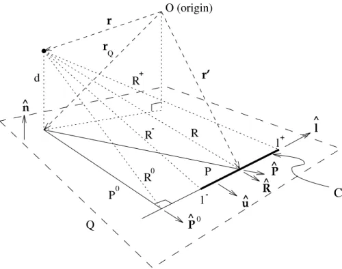
Related geometric quantities associated with an edge Ci of S in the plane containing S, Q,

are shown in Figure 2.3 for r0_{∈ C}

i. Without loss of generality, it is assumed that

d∆₌n·(r − rˆ 0_{) > 0} _(2.14)

which is equal to the distance from r to Q. For (i), we have (see [1])

(25)

l P R u P n P d ^ ^ ^ ^ ^ R r r’ l -l+ 0 R0 0 P r Q R -+ Q R O (origin) C ^

Figure 2.3: Geometric quantities associated with a point, an edge Ci (subscript i is omitted)

of S shown in Figure 2.2 and the plane Q containing S.

1

Rm = ∇S·(fm(R)P) (2.15)

where P is the position vector of r0 _{with respect to the projection of r on Q, r} Q, and fm(R)=        log R R2_{− d}2, m = 2 −1 (m − 2)Rm−2_(R2_{− d}2₎. m 6= 2 (2.16)

Note that if rQ is inside S, fm(R) will become singular for some r00 = rQ, i.e., R = d.

Let Sεdenote the intersection of S and a small circular region on Q of radius ε and centered

at rQ, the potential due to S can be evaluated as

Z S dS Rm = lim_ε→0 "Z S−Sε ∇s·(fm(R)P)dS+ Z Sε dS Rm # (2.17) = Z ∆Sfm(l)P· ˆudl + limε→0 "Z _α 0 Z _ε 0 pdpdθ (p2_+d2₎m2 # = X i Pi0·ˆui Z Ci fm,i(li)dli+ gm(α), where fm,i(li) = fm(R = q li2 + d2+ (Pi0)2), (2.18)

(26)

gm(α) =    α log d, m = 2 α (m − 2)dm−2, m > 2 (2.19)

Pi0 is the distance between rQ and Ci, li is measured from the projection of r on Ci along

the direction of ˆli, and α is the angular extent of the circumference of Sε lying inside S as

ε → 0. For example, α = 2π if rQ is inside S, α = π if rQ is on an edge of S and α is equal

to the angle between two edges if rQ is a vertex of S where the two edges are connected.

Since fm,i(li) is a rational function for even m’s when m 6= 2 and is rationalizable for

odd m’s (see [52]), the line integrals can always be evaluated in closed form except for m = 2. For example, if Pi0 6= 0, we have2

Z Ci f3,i(li)dl = Z _l_i+ li− f3,i(li)dl = 1 Pi0d " tan−1 li −_d Pi0R− −tan−1 li +_d Pi0R+ # . (2.20)

with R− _{and R}+ _{equal to the distances from r to the two end points of C}

i, respectively.

Thus, the repulsive force exerted on a point charge at (x, y, z) due to polygon j, denoted as

Φ(x, y, z) =X

i

[φ(xi₂, yi₂, z) − φ(xi₁, y₁i, z)] + α

z, (2.21)

can be obtained analytically by evaluating the gradient of the potential function for m = 3 with

φ(x, y, z) = 1 ztan

−1 xz

y√x2_{+ y}2_{+ z}2 (2.22)

where the xi− yi− z coordinate system is determined by the right-hand rule for each edge i

of the polygon such that z is measured along the normal direction and xi is measured along

edge i of the polygon, respectively.

2.2.2 Integral Equation of Repulsion

Therefore, the repulsive force at point (x, y, z) due to polygon j can be denoted as

fj _{= (f}j x, fyj, fzj) = ( ∂Φj ∂x , ∂Φj ∂y , ∂Φj ∂z ) (2.23)

For the potential-based path planning of manipulators, the evaluation of the repulsion between manipulators and obstacles involves the calculation of the repulsion between pairs

2_{Detailed discussions concerning some special cases for the potential calculation, e.g., for P}

i0 = 0 or

d = 0, etc., as well as the associated collision avoidance property can be found in [1]. In this thesis, only m = 3 is considered.

(27)

Figure 2.4: The sampling model for a link of a manipulator.

of polygons; each pair has a polygon from the manipulator and the other from obstacles. To simplify the mathematics, links of manipulator are approximately represented by a set of point samples on their surfaces in this thesis. Usually, as shown in Fig. 2.4, the sampling points are located on the vertexes and edges of links and their distribution should be as uniform as possible.

Assume that a link has m point samples and the obstacles have n polygon surfaces. If the repulsive force between point sample pk and surface Sj is denoted as fkj, the repulsive

force exerted on p is equal to

fk = ( n X j f_kj_x, n X j f_kj_y, n X j f_kj_z) (2.24)

according to (11), and the total repulsive force exerted on the link can be evaluated as

f =

m

X

k

fk. (2.25)

The repulsion expressed by (2.25) will be used in the potential-based path planning for robot manipulators in 3-D workspace, as discussed next. The total repulsive torque exerted on a link with respect to a point, say a joint, can be derived similarly, which is omitted for brevity.

(28)

Chapter 3 Potential-based Path Planning in 2-D

Environments

3.1 Overview

Path planning of a manipulator is to determine a collision-free trajectory from its original location and orientation (called starting configuration) to the goal configuration [53]. Some planners adopt the configuration space (c-space) base approach [3] [4] [5] [6] [7] [15]. A point in a c-space indicates a configuration of manipulator which is usually encoded by a set of manipulator’s parameters; e.g., joint angles between manipulator links. Then, path planning of a robot is reduced to the problem of planning a path of a point in free space of the c-space. The performance of c-space approaches is usually restricted by the exponential growth of computation with robot degrees of freedom. Unlike c-space based approaches, geometric algorithms directly use spatial occupancy information of the workspace (w-space) to solve path planning problem [8] [9] [1] [10] [11] [12] [14] [13] [2]. Workspace-based algorithms usually extract relevant information about the free space and use them together with the manipulator geometry to find a path. However, not all approaches try to find path with minimum risk of collision. To minimize such a risk, repulsive potential fields between charged manipulator and obstacles are used in [9] [11] [12] and [13] to match their shapes in the path planning.

In this thesis, the potential field model presented in [13], as reviewed in the next sec-tion, is adopted to model the workspace for the path planning of robot manipulators. A collision-free path of a manipulator will then be obtained by locally adjusting the manip-ulator configuration to search for minimum potential configurations using these force and torque. The proposed approach uses one or more guide lines (GLs) among obstacles in the

(29)

free space as final or intermediate goals in the workspace for a manipulator to reach. These GLs provide the manipulator a general direction to move forward and also help to establish certain motion constraints for adjusting manipulator configuration during path planning, as discussed in Section 3.2. In Section 3.3, the implementation details are given. In Section 3.4, simulation results are presented for path planning performed on SUN workstation for manipulators in 2-D environment. Section 3.5 gives conclusions of this chapter.

3.2 A Potential-Based Path Planning algorithm in 2-D

Environments

The application of the potential model reviewed in the previous section for path planning of manipulators will be discussed in this section. For a rough description of object path, the proposed approach uses one or more guide lines (GLs) as final or intermediate goals in the workspace. The GLs are line segments among obstacles in the free space, providing the manipulator a general direction to move forward (see Fig. 3.1). A collision-free traversal of a given sequence of GLs by the end-effector is regarded as a global solution of the path planning problem of a manipulator. Although free space bottlenecks which are defined by minimal distance links (MDLs) among the obstacles are good candidates as GLs for path planning1_{, other links among the obstacles can also be used, e.g., GL}

3 shown in Fig. 3.1.

GL

1

GL

2

GL

3

Figure 3.1: A manipulator is moved toward the goal (not shown) by sequentially traversing a sequence of GLs.

3.2.1 Basic procedure of path planning

The proposed path planning approach derives a series of minimum potential configurations along the path of a manipulator by locally adjusting its configuration for minimum potential

1_{For example, MDLs are used to connect (convex) obstacle nodes in the obstacle neighborhood graph in}

(30)

δ p' e1 e2 p GL e1 e2 p GL e1 e2 GL p (a) (b) (c)

Figure 3.2: Basic planning procedure for a given GL.

using the results given in Sec. 2. Assuming that a guide line e1e2 is given as an intermediate

goal, the basic path planning procedure for moving the end-effector p of a manipulator onto

e1e2 includes (see Fig. 3.2):

(i) Translate the distal links of the manipulator to move p toward the e1e2. (Fig. 3.2(a))

(ii) For constant |pe1| + |pe2|, repeatedly execute :

(a) Search for the minimum potential configuration of the manipulator with the distal link fixed in orientation. (Fig. 3.2(b))

(b) Search for the minimum potential configuration of the manipulator with p fixed in position. (Fig. 3.2(c))

(iii) Repeat (i) and (ii) until the end-effector reaches the line segment e1e2.

In general, there are different ways to change the manipulator configuration to move p toward e1e2. A simple translation of distal links is adopted in (i). As shown in Fig. 3.2(a),

the translation of a predetermined distance δ of the distal link is carried out to move the end-effector from p0 _{to p. The direction of the translation is determined with respect to e}

1

and e2 such that

−→

p0_{p bisects} ₆ _e

1p0e2. If there is a collision, each time the distance of the

translation is reduced by 50% until it is collision-free. No configuration improvement using the repulsion experienced by the manipulator is considered at this stage.

(31)

In (ii), the associated constrained optimization problem is divided into two iterative univariant optimization procedures, as in (ii-a) and (ii-b). In (ii-a), the distal link is fixed in its orientation (see Fig. 3.2(b)) as p slides along the elliptic trajectory to search for the minimal potential configuration and other distal links are sequentially adjusted in orienta-tion, staring from the link connected to the distal link. In (ii-b), the distal link is adjusted in orientation while fixed in position (see Fig. 3.2(c)) and the procedure for adjusting the rest links is similar to that in (ii-a). Detailed implementation is presented in next section.

For each elliptical trajectory, (ii-a) and (ii-b) are repeatedly performed until negligi-ble changes in the manipulator configuration are obtained. Then another smaller elliptical trajectory is obtained with (i) and the process repeats. The path planning algorithm, as summarized below, ends as the end-effector reaches the given GL.

Algorithm End Effector to GL

Step 0 Initialize δ = δ0, where δ0 is arbitrarily chosen.

Step 1 Translate the manipulator with distance δ along the direction of the bisector vector of −−→p0_e

1 and

−−→ p0_e

2. If collision occurs or if the two base links become unconnected,

δ ←− δ/2 and go to Step 1.

Step 2 Translate the distal link to move p along the elliptical trajectory, |pe1| + |pe2| =

constant, to minimize the potential.

Step 3 Joint angle adjustment for the minimum potential configuration with p fixed in position.

Step 4 Go to Step 2 if the translation in Step 2 or the joint angle adjustment in Step 3 is not negligible.

Step 5 If p reaches GL, the planning is completed. Otherwise, go to Step 1 with δ = δ0.

For path planning involving multiple GLs, the above algorithm will be executed for each of them sequentially. It is assumed that the planning for a GL starts as the planning of the previous GL is accomplished. The path planning ends as the end-effector reach the goal, which is usually a (goal) GL in the path planning problems considered in this thesis.

(32)

3.3 Implementation details

3.3.1 Step 1 of END EFFECTOR TO GL

Consider the manipulator shown in Fig. 3.2(a). Its end-effector is initially located at point

p0 _{and is moved toward an intermediate goal GL, such that it is moved with distance δ}

along the direction of the bisector vector of −−→p0_e

1 and

−−→ p0_e

2, from p0 to p. Such a movement

is achieved in the implementation by translating every link except the two base links. It is not hard to see that the two base links have at most two possible configurations; i.e., the two base links together may have two, one, or no feasible configurations depending on the amount of translations of the distal links. In the computer implement, if there are two feasible configurations for the two base links, the one requiring less adjustments in joint angles of the two links is selected.

3.3.2 Implementation of Step 2

In Step 2, since the minimization is constrained by |pe1|+|pe2| = constant, only the resultant

force experienced by the distal link along the tangential direction of the ellipse is taken into account. Consider the forces exerted on the distal link lnkn, as shown in more detail in

Fig. 3.3. Let f1 be the repulsive force exerted on lnkn due to the repulsion between lnkn

and the obstacles, and f2 be the force exerted on Jn−1 due to the repulsive torque between

other manipulator links and obstacles. For a univariant minimization approach, only one variable is adjusted at a time. To determine the minimum potential location of lnkn under

the elliptical constraint, all of the joint angles of the manipulator, except the base joint J0,

are assumed to be fixed. Therefore, the above repulsive torque, denoted as τ0, is calculated

for a single rigid composite link formed by all the other manipulator links with respect to

J0. Thus, we have

f2 =

τ0

l0

(3.1) where l0 is the length of J0Jn−1.

To determine the direction in which p should slide along the ellipse E1, and thus lnkn

should translate, to reduce the repulsive potential, the direction of the projection of the resultant force exerted on lnkn along the tangent of E1 at p, L,

(33)

e

1

e

2

p

lnk

n

J

L

L guideline guideline

f

₁

f

₂ Base Joint guideline

f

J

₀ n-1

E

1

Figure 3.3: Sliding p along ellipse E1, by translating lnkn to reduce the repulsive potential.

is calculated. A gradient-based binary search for the minimum potential location of p along

E1 can thus be performed using (14). The search ends when the movement of lnkn or the

magnitude of fL is negligible.

Each time the position p, and lnkn, is changed in the above search process, the

orienta-tion of rest links, i.e., joint angles at J0 through Jn−1, need to be adjusted for connectivity

and for minimum potential of the manipulator. Such a procedure is very similar to the joint angle adjustment performed in Step 3, as discussed next.

3.3.3 Adjusting joint angles in Step 3

Once the minimum potential position of distal link is determined with Step 2, another univariant procedure, which allows the distal link to adjust its orientation but not its location, is performed to reduce the potential further, as shown in Fig. 3.2(c). Under the constraint that end-effector is fixed in location p, the distal link can rotate with respect to p to reduce the repulsive potential. The direction in which the distal link should rotate is determined by the repulsive torque experienced by the distal link with respect to p.

Consider the repulsion experienced by the distal link lnkn with end-effector p fixed in

position. Let τn be the repulsive torque experienced by lnkn with respect to p due to the

repulsion between lnkn and let f2, as described in the previous subsection, be the force

exerted on Jn−1 due to the repulsive torque between other manipulator links and obstacles.

The resultant torque experienced by lnkn with respect to p is equal to

(34)

where lnis the length of lnknand f2⊥is the projection of f2along the direction perpendicular

to lnkn. A gradient-based binary search for the minimum potential orientation of lnkn for p

fixed in position can thus be performed using the direction of τn∗. Each time the orientation

of lnkn is changed , the orientation of the rest links are adjusted iteratively for connectivity

and for minimum potential using τn−1∗, τn−2∗, ...., etc. The search ends when the movement

of lnkn or the torque τn∗ is negligible.

3.4 Simulation Results

In this section, simulation results are presented for path planning performed on SUN Ultra−1 for manipulators in 2-D environment. In order to show the path of a manipulator more clearly, every configuration of a path obtained by End Effector to GL is shown in different gray level, i.e., the initial configuration is shown in black and final configuration is shown in white. Moreover, all manipulator and obstacle boundaries are assumed to be uniformly charged, except for those marked out explicitly for non-uniform charge distributions. The precisions for optimal configurations obtained in Steps 2 and 3 are equal to 0.3 units and 0.625o_{, respectively, for link locations and orientations.}

Fig. 3.4 shows the path planning result similar to an example shown in [54]. In our simulation, there are two GLs predetermined in the workspace of size 30 by 20 units. The initial distance of translation, δ0, is arbitrarily chosen as 2.2 units. The simulation takes a

total of 5.66 seconds to plan the 11-configuration collision-free path and spends most CPU times for the first and seventh configurations. The planned manipulator path is observed to achieve better results in terms of collision avoidance compared with the path obtained in [54]. Fig. 3.5 shows the path planning result similar to an example shown in [55]. In our simulation, there are four GLs predetermined in the workspace of size 30 by 30 units. The initial distance of translation, δ0, is chosen as 4.0 units. While it takes five seconds for a

SUN SPARC to generate a 4-configuration path in [55], the 8-configuration path is obtained by the proposed algorithm in 0.87 seconds for a SUN Ultra−1.

In general, the number of configuration and the computation time depend on the size of the initial distance of translation, δ0. For larger δ0, less configurations will be generated along

the path if there is no collision. On the other hand, if δ0 is too large, the computation time

(35)

Figure 3.4: A path planning example derived from [54].

Figure 3.5: A path planning example derived from [55].

similar to an example shown in [7]. In our simulation, there are seven GLs predetermined in the workspace of size 30 by 20 units. The initial distance of translation, δ0, is chosen

as 2.2 units. The simulation takes a total of 5.5934 seconds to plan the 16-configuration collision-free path. Different values of δ0, from 0.5 to 2.4 units, are also simulated, and the

simulations take 6.26 to 16.48 seconds. For the PRM presented in [7] using a DEC Alpha, a computation time of 5 seconds corresponds to success rates of 50%. For a success rate of more than 97%, the total computation time will exceed 15 seconds.

The proposed algorithm is also performed well for high DOF manipulators. Fig. 3.7(a) shows a high DOF example in which a 9-link manipulator need to snake into the cave with a collision-free path. There are four GLs predetermined in the workspace of size 30 by 30 units. The initial distance of translation, δ0, is chosen as 2.2 units. The computation time

(36)

Figure 3.6: A various δ example derived from [5].

of the 11-configuration path takes a total of 9.26 seconds. In Fig. 3.7(a), the manipulator may moves very close to an obstacle’s corner (as indicated with a pointer). In order to keep a safe distance away from the corner, the charge distributions of the left side of the cave is modified to be non-uniform and a safer manipulator path is obtained, as shown in Fig. 3.7(b). In Fig. 3.7(b), the charge density is doubled for the segment marked with three 2’s and is increased linearly from 1 to 2 for another marked segment. The computation time is equal to 12.4 seconds for the path shown in Fig. 3.7(b).

3.5 Summary

In this thesis, a potential-based algorithm for the path planning of a robot manipulator is proposed. The proposed algorithm uses an artificial potential field to model the workspace wherein object boundaries are assumed to be charged with various source distributions. Simulation results show that a path thus derived is always spatially smooth while its safety level can be adjusted easily by selecting proper charge distributions for the potential-based workspace model. Since the proposed approach uses workspace information directly, it is readily applicable to manipulators of high DOFs. In our experiments, manipulators with DOFs up to 9 have been tested with satisfactory results.

(37)

(a) uniform charge (b) non-uniform charge

(38)

Chapter 4 Potential-based Path Planning of

Manipulator in 3-D Environments

4.1 Overview

In this chapter, the potential field model presented in [1] is adopted to model the workspace for the path planning of robot manipulators. The approach is similar to that done in 2-D manipulator mentioned in Chapter 3, except the 2-DOFs of joints and adopted potential model. In a 3-D environment, the proposed approach uses one or more guide planes (GPs) instead of guide lines (GLs) among obstacles in the free space as final or intermediate goals in the workspace for the manipulator to reach. These GPs provide the manipulator a general direction to move forward and also help to establish certain motion constraints for adjusting manipulator configuration during path planning, as discussed in Section 4.2. The algorithm proposed in Section 4.2 has similar steps as the one in Section 3.2.1. The implementation details are given in Section 4.3. In Section 4.4, simulation results are presented for path planning performed for manipulators in different 3-D environments. Section 4.5 gives a conclusion of this work.

4.2 The Proposed Path Planning Algorithm

The application of the potential model reviewed in the previous section for path planning of manipulators will be discussed in this section. Unlike some c-space based approaches, which often require expensive preprocessing to construct the c-space, the proposed approach uses the workspace information directly. The approach computes repulsive force and torque experienced by each rigid component, e.g., a link, of a manipulator. A collision-free path of the manipulator can then be obtained by locally adjusting its configuration along the path

(39)

GP1 GP2 (a) GP1 GP2 (b)

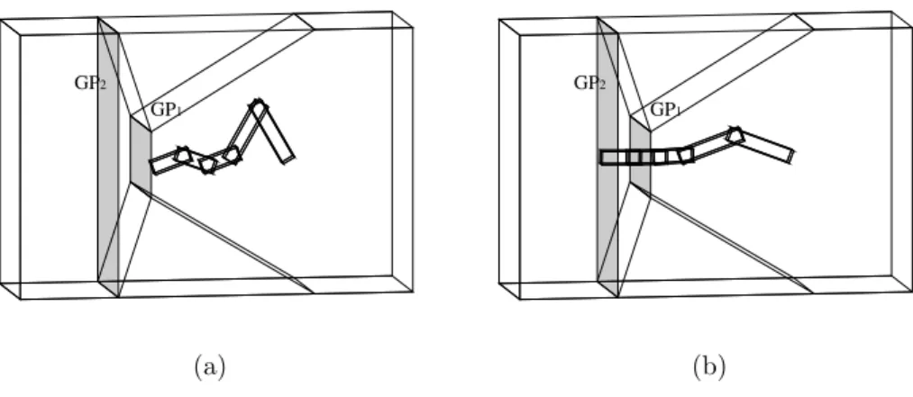
Figure 4.1: A manipulator is moved toward the goal (not shown) by sequentially traversing a sequence of GPs.

(a) (b)

Figure 4.2: The generalized cylinder presentation of a passage.

for minimum potential using these force and torque. In this thesis, the spherical joint is adopted to connect links of a manipulator since its high DOFs can take full advantage of the proposed potential minimization algorithm.

For a rough description of manipulator path, the proposed approach uses one or more guide planes (GPs) as final or intermediate goals in the 3-D workspace. The GPs are polygons among obstacles in the free space, providing the manipulator a general direction to move forward (see Fig. 4.1). A collision-free traversal of a given sequence of GPs by the end-effector is regarded as a global solution of the path planning problem of a manipulator.

(40)

4.2.1 Generation and Selection of initial GPs

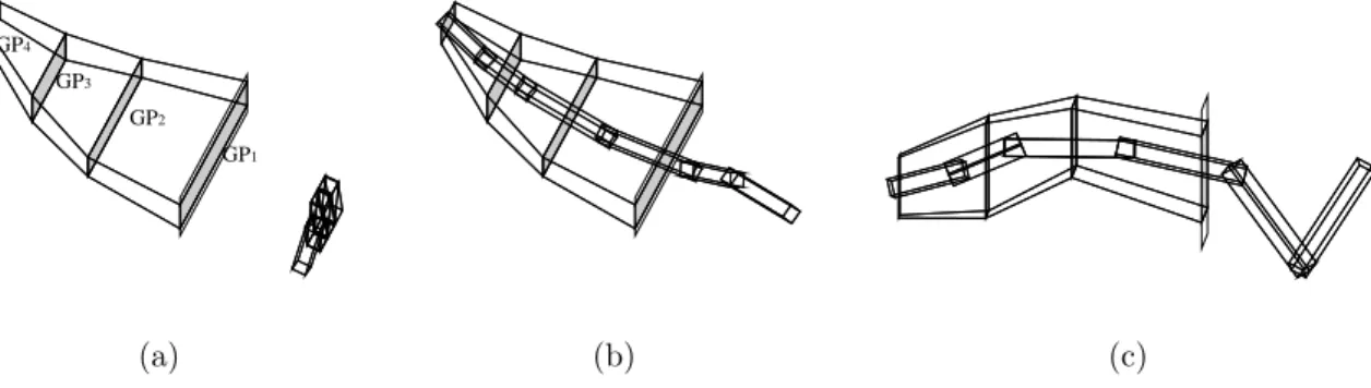
In the proposed algorithm, the GPs provide the articulated robot a general direction to move forward. The selection of the initial GPs may base on (i) their density along the passage, (ii) the visibility between two adjacent GPs, or (iii) the angular variation of two adjacent GPs. For the examples considered in this chapter, the initial GPs are selected arbitrarily and the algorithm seems to work reasonably well in terms of the sensitivity of the planned path to the selection of initial GPs. Often, these initial GPs can also be obtained from the Generalized Cylinder (GC) [56] representation as cross-sections perpendicular to the GC axis. Figs. 4.2(a) shows a passage which has approximately rectangular cross-sections, and an axis of its GC representation. In general, there is no limit on the number of cross-sections and their shapes are not explicitly specified in advance. More details about generalized cylinder representation can be found in Appendix A.

In the proposed approach, the shape of the GPs is usually not critical as long as the GPs are confined in the free space. In face, only the normal direction of a GP, e.g., the direction of the GC axis, is important. Such an axial representation can also be derived from (i) the global navigation function as in [57][5][58], as well as (ii) the tree structure representation of free space obtained from the wavefront expansion presented in [59]. While the gradient of (i) leads a point object to the goal, global connectively of free space is available in (ii) and is used in [59] to solve a planning problem in low dimensions.

4.2.2 Basic Procedure of Path Planning

In this chapter, the proposed path planning approach derives a series of minimum potential configurations along the path of a manipulator by locally adjusting its configuration for minimum potential using the results given in Sec. 2.2. Assuming that a guide plane GP1 is

given as an intermediate goal, the basic path planning procedure for moving the end-effector

p0 _{of a manipulator onto GP}

1 include (see Fig. 4.3):

(i) Translate the distal links1 _{of the manipulator to move its end-effector p}0 _{toward the GP}

1.

If p0 _{can not reach GP}

1 directly, e.g., due to collision, a virtual intermediate plane GP10

1_{In step (i), an intermediate simple solution of the inverse kinematics problem is obtained by translating}

of all manipulator links except for the two base links, the base link and the link connected to it. For each translation, the two base links, together, can have at most three DOFs. In step (ii), the problem is solved by finding a sequence of sub-optimal solutions with monotonically decreasing potential. Finally, the minimal potential solution is found in (iii).

利用位能場模型作路徑規劃及物體形狀比對

國立交通大學

資訊科學研究所

博士論文

利用位能場模型作路徑規劃及物體形狀比對

Potential-Based Path Planning and Shape

Matching

研 究 生：林建州

指導教授：莊仁輝 博士

利用位能場模型作路徑規劃及物體形狀比對

Potential-Based Path Planning and Shape Matching

研

究

生：林建州 Student：Chien-Chou Lin

指導教授：莊仁輝

Advisor：Jen-Hui Chuang

國立交通大學

電機資訊學院

資訊科學研究所

博士論文

A Thesis

Submitted to Institute of Computer and Information Science

College of Electrical Engineering and Computer Science

National Chiao Tung University

in Partial Fulfillment of the Requirements

for the Degree of Doctor of Philosophy

in

Computer and Information Science

September 2004

Hsinchu, Taiwan, Republic of China

利用位能場模型作路徑規劃及物體形狀比對

研究生：林建州

指導教授：莊仁輝 博士

國立交通大學資訊科學研究所

摘要

Potential-Based Path Planning and Shape Matching

Student：Chien-Chou Lin

Advisor：Dr. Jen-Hui Chuang

Institute of Information and Computer Science

National Chiao Tung University

Abstract

Contents

List of Figures

Chapter 1

Introduction

1.1

Motivation

1.2

Survey of Path Planning in 2-D Environments

1.3

Survey of Path Planning in 3-D Environments

1.4

Survey of Shape Matching of 3-D Objects

1.5

Organization of the Thesis

Chapter 2

Reviews of Adopted Potential Models

2.1

A Review of the 2-D Potential Model

2.1.1

Repulsion due to Charged Polygonal Region Borders

2.1.2

Integral equations for forces and torques

2.1.3

Repulsion due to linear and quadratic charge distributions

2.2

A Review of the Generalized 3-D Potential Model

2.2.1

Integral Equation of 3-D Potential Modeling

2.2.2

Integral Equation of Repulsion

Chapter 3

Potential-based Path Planning in 2-D

Environments

3.1

Overview

3.2

A Potential-Based Path Planning algorithm in 2-D

Environments

GL

研究生：林建州

指導教授：莊仁輝博士

指導教授：莊仁輝博士