國
立
交
通
大
學
資訊工程學系
碩
士
論
文
利用迴歸分析於探勘使用者移動模式
Exploring Regression for Mining User Moving Patterns in a Mobile
Computing System
研 究 生:洪智傑
指導教授:彭文志 教授
利用迴歸分析探勘使用者移動樣式於行動計算系統
Exploring Regression for Mining User Moving Patterns in a Mobile
Computing System
研 究 生:洪智傑 Student:Chih-Chieh Hung
指導教授:彭文志 Advisor:Wen-Chih Peng
國 立 交 通 大 學
資 訊 工 程 學 系
碩 士 論 文
A ThesisSubmitted to Department of Computer Science and Information Engineering National Chiao Tung University
College of Eletrical Engineering and Computer Science in partial Fulfillment of the Requirements
for the Degree of Master
in
Computer Science and Information Engineering May 2005
Hsinchu, Taiwan, Republic of China
博碩士論文授權書
本授權書所授權之論文為本人在__交通____大學(學院)_資訊工程___系所 _______組__九十三__學年度第_二__學期取得_碩_士學位之論文。 論文名稱:_利用迴歸分析探勘使用者移動樣式於行動計算系統__ 指導教授:_彭文志_____________________ 1.■同意 □不同意 本人具有著作財產權之上列論文全文(含摘要)資料,授予行政院國家科學委員會科學技 術資料中心(或改制後之機構),得不限地域、時間與次數以微縮、光碟或數位化等各種 方式重製後散布發行或上載網路。 本論文為本人向經濟部智慧財產局申請專利(未申請者本條款請不予理會)的附件之 一,申請文號為:______________,註明文號者請將全文資料延後半年再公開。 2. ■同意 □不同意 本人具有著作財產權之上列論文全文(含摘要)資料,授予教育部指定送繳之圖書館及國 立交通大學圖書館,基於推動讀者間「資源共享、互惠合作」之理念,與回饋社會及學 術研究之目的,教育部指定送繳之圖書館及國立交通大學圖書館得以紙本收錄、重製與 利用;於著作權法合理使用範圍內,不限地域與時間,讀者得進行閱覽或列印。 本論文為本人向經濟部智慧財產局申請專利(未申請者本條款請不予理會)的附件之 一,申請文號為:______________,註明文號者請將全文資料延後半年再公開。 3. ■同意 □不同意 本人具有著作財產權之上列論文全文(含摘要),授予國立交通大學與台灣聯合大學系統 圖書館,基於推動讀者間「資源共享、互惠合作」之理念,與回饋社會及學術研究之目 的,國立交通大學圖書館及台灣聯合大學系統圖書館得不限地域、時間與次數,以微縮、 光碟或其他各種數位化方式將上列論文重製,並得將數位化之上列論文及論文電子檔以 上載網路方式,於著作權法合理使用範圍內,讀者得進行線上檢索、閱覽、下載或列印。 論文全文上載網路公開之範圍及時間 – 本校及台灣聯合大學系統區域網路: 年 月 日公開 校外網際網路: 年 月 日公開 上述授權內容均無須訂立讓與及授權契約書。依本授權之發行權為非專屬性發行權利。依本 授權所為之收錄、重製、發行及學術研發利用均為無償。上述同意與不同意之欄位若未鉤選, 本人同意視同授權。 研究生簽名: 學號:9217582 (親筆正楷) (務必填寫) 日期:民國 94 年 5 月 24 日 1. 本授權書請以黑筆撰寫並影印裝訂於書名頁之次頁。
國家圖書館博碩士論文電子檔案上網授權書
本授權書所授權之論文為本人在__交通__大學(學院)___資訊工程___系所 _______組__九十三___學年度第_二_學期取得_碩_士學位之論文。 論文名稱:_利用迴歸分析探勘使用者移動樣式於行動計算系統___ 指導教授:彭文志__________________________ ■同意 □不同意 本人具有著作財產權之上列論文全文(含摘要),以非專屬、無償授權國家圖書館,不限地域、 時間與次數,以微縮、光碟或其他各種數位化方式將上列論文重製,並得將數位化之上列論 文及論文電子檔以上載網路方式,提供讀者基於個人非營利性質之線上檢索、閱覽、下載或 列印。 上述授權內容均無須訂立讓與及授權契約書。依本授權之發行權為非專屬性發行權利。依本 授權所為之收錄、重製、發行及學術研發利用均為無償。上述同意與不同意之欄位若未鉤選, 本人同意視同授權。 研究生簽名: 學號:9217582 (親筆正楷) (務必填寫) 日期:民國 94 年 5 月 24 日 1. 本授權書請以黑筆撰寫,並列印二份,其中一份影印裝訂於附錄三之一(博碩士論 文授權書)之次頁﹔另一份於辦理離校時繳交給系所助理,由圖書館彙總寄交國家 圖書館。Ackowledgement
I spent a lot of time thinking about writing this part of the dissertation. There are many people I would like to thank and many of them have an influence on my life and this dissertation. In order to reach the point of writing this dissertation, I conducted several research works under the supervision of my advisor Prof. Dr. Wen-Chih Peng. His overly enthusiasm and integral view on research has made a deep impression on me. I am also grateful for the inter-esting interactions and discussions we had during the two years I spent in National Chiao Tung University. With his constant guidance, timely encouragement and unwavering support, I have learned research capabilities and finished my dissertation. I always keep his advice: ’not pleased by external gains, not saddened by personal losses.’ Besides of being an excellent advisor, he was as close as a relative and a good friend to me. I owe him lots of gratitude for having me shown this way of research and his care.
I also want to thank my committee members, Prof. Suh-Yin Lee, and Prof. Ming-Syan Chen, or all the comments. They made on this dissertation and also during my oral defence.
During the two years, I have also received encouragement from many friends and the members in Advanced Database System Laboratory. I want to thank my best friend Wan-Chun Yin. The solution procedures of this research work suddenly appeared in my brain when we had a talk. I will never forget the wonderful moment when I tasted the happiness of thinking. Also, the members in ADSLab gave me a pleasant atmosphere to do research, and I also indeed appreciate their friendship and cherish the time when we are together. At last, I would like to give particular thanks to Chun-Ling Lin for supporting me throughout this work, and in particular during the stressful writing-up period. Life would have been very difficult without you. Thanks for your consideration and thoughtfulness.
Finally, I could not reach the important milestone of my life without the support of my family. Thanks to my parents who have made it possible for me to reach where I am now standing. This dissertation is dedicated to them.
Abstract
In this thesis, by exploiting the log of call detail records, we present a solution procedure of mining user moving patterns in a mobile computing system. Specifically, we propose algorithm LS to accurately determine similar moving sequences from the log of call detail records so as to obtain moving behavior of users. By exploring the feature of spatial-temporal locality, which refers to the feature that if the time interval among consecutive calls of a mobile user is small, the mobile user is likely to move nearby, we develop algorithm TC to cluster those call detail records whose time intevals are very close. In light of the concept of regression, we devise algorithm MF to derive moving functions of moving behavior. Performance of the proposed solution procedure is analyzed and sensitivity analysis on several design parameters is conducted. It is shown by our simulation results that user moving patterns obtained by our solution procedure are of very high quality and in fact very close to real user moving behavior.
Contents
1 Introduction 1
2 Related Works 7
2.1 Generation of Moving Log . . . 7
2.2 Incremental Mining for Moving Patterns in a Mobile Environment . . . 8
2.2.1 Finding Maximal Moving Sequences . . . 9
2.2.2 Finding Large Moving Sequences . . . 11
3 Mining User Moving Patterns 15 3.1 Preliminary . . . 15
3.2 Procedure for Mining User Moving Patterns . . . 17
3.2.1 An Overview . . . 17
3.2.2 Data Collection Phase . . . 18
3.2.3 Time Clustering Phase . . . 21
3.2.4 Regression Phase . . . 27
4 Performance Study 35 4.1 Simulation Model for a Mobile System . . . 35
4.2 Experiments of UMP and AUMP . . . 37
4.3 Sensitivity Analysis of AUMP . . . 38
List of Figures
1.1 A moving path and an approximate user moving pattern of a mobile user . . . 4 3.1 An illustrative example, where the arrow line is the real moving path and the solid
line is estimated by moving functions obtained by algorithm MF. . . 31 3.2 A snapshot of complete moving function F (t) . . . 33 3.3 An illustrative example for transformation from geometric model to symbolic model 34 4.1 The precise ratio of UMP and AUMP with the value of mf varied. . . 37 4.2 The cost ratios of AUMP and UMP with the moving frequency varied . . . 38 4.3 The performance of AUMP with the value of w varied. . . 39 4.4 The precise ratio of AUMP with vertical_min_sup and match_min_sup varied. 39 4.5 The precise ratio of AUMP with the values of match_min_sup and the variance
threshold varied. . . 40 4.6 The precise ratio of AUMP with the values of vertical_min_sup and variance
List of Tables
1.1 An example of selected call detail records. . . 2
2.1 An illustrative example for algorithm MM . . . 10
2.2 An example for counting the occurrences of 2-moving sequences . . . 13
3.1 An example of algorithm LS . . . 21
3.2 An execution scenario under algorithm TC. . . 26
3.3 Data points with their corresponding weights. . . 30
Chapter 1
Introduction
Due to recent technology advances, an increasing number of users are accessing various infor-mation systems via wireless communication. Such inforinfor-mation systems as stock trading, banking, wireless conferencing, are being provided by information services and application providers[3][5][9][11], and mobile users are able to access such information via wireless communication from anywhere at any time [16][22].
User moving patterns are referred to the areas where users frequently travel in a mobile computing environment. It is worth mentioning that user moving patterns are particularly important and are able to provide many benefits in mobile applications. A significant amount of research efforts has been elaborated upon issues of utilizing user moving patterns in developing location tracking schemes and data allocation methods [7][15]. We mention in passing that the authors in [7] developed a new location tracking strategy based on user moving behaviors. The authors in [15] devised data allocation schemes that are able to allocate data to the areas defined according to user moving patterns. Clearly, user moving patterns are beneficial on developing
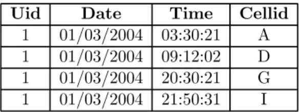
Uid Date Time Cellid
1 01/03/2004 03:30:21 A
1 01/03/2004 09:12:02 D
1 01/03/2004 20:30:21 G
1 01/03/2004 21:50:31 I
Table 1.1: An example of selected call detail records.
location management and querying strategy in a mobile computing system [7][15][18][20][21]. Thus, it has been recognized as an important issue to develop algorithms to mine user moving patterns so as to improve the performance of mobile computing systems.
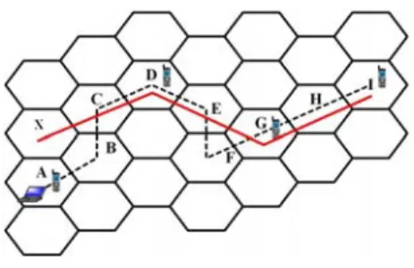
The study in [15] explored the problem of mining user moving patterns with the moving log of mobile users given. Specifically, in order to capture user moving patterns, a moving log recording each movement of mobile users is needed. In practice, generating the moving log of all mobile users unavoidably leads to the increased storage cost and degraded performance of mobile computing systems. Consequently, in this paper, we address the problem of mining user moving patterns from the existing log of call detail records (referred to as CDR) of mobile computing systems. Generally, mobile computing systems generate one call detail record when a mobile user makes or receives a phone call. Table 1.1 shows an example of selected real call detail records where Uid is the identification of an individual user that makes or receives a phone call and Cellid indicates the corresponding base station that serves that mobile user. Thus, a mobile computing system produces daily a large amount of call detail records which contain hidden valuable information about the moving behaviors of mobile users. Unlike the moving log keeping track of the entire moving paths, the log of call detail records only reflects the fragmented moving behaviors of mobile users. However, such a fragmented moving behavior is of little interest in
a mobile computing environment where one would naturally like to know the complete moving behaviors of users. Thus, in this paper, with these fragmented moving behaviors hidden in the log of call detail records, we devise a solution procedure to mine user moving patterns. The problem we shall study can be best understood by the illustrative example in Figure 1.1 where the log of call detail records is given in Table 1.1. The dotted line in Figure 1.1 represents the real moving path of the mobile user and the cells with the symbol of a mobile phone are the areas where the mobile user made or received phone calls. Explicitly, there are four call detail records generated in the log of CDRs while the mobile user travels. The corresponding locations of these call detail records are scattered over the mobile computing environment, showing the limited information obtained from the log of CDRs when it comes to mining user moving patterns. Given these fragmented moving behaviors, we explore the technique of regression analysis to generate approximate user moving patterns (i.e., the solid line in Figure 1.1). As shown in Figure 1.1, the approximate user moving pattern (i.e., the solid line) is very close to the real moving behavior (i.e., the dotted line). In practice, approximate user moving patterns are able to provide sufficient user moving behaviors. For example, some mobile applications only require the moving trend of users. Furthermore, if approximate user moving patterns are close to the real moving paths, one can utilize approximate user moving patterns to predict the real moving behaviors of mobile users. Consequently, given the log of call detail records, we shall develop in this paper an efficient approach of mining user moving patterns close to real moving behaviors.
In this paper, we propose a regression-based solution procedure to mine user moving patterns. Regression analysis is widely applied in many scientific fields including statistics, economy, bi-ological informatics and data mining. The main objective of regression analysis is that given
Figure 1.1: A moving path and an approximate user moving pattern of a mobile user data points, a regression line is calculated with the purpose of minimizing the distance between the line derived and data points. Therefore, regression analysis is very suitable to mine user moving patterns with call detail records given. Compared to the moving log, call detail records reflect fragmented moving behavior of mobile users and thus call detail records are very precious for mining user moving patterns. However, the moving behavior of mobile users may scatter widely, making the traditional regression analysis not directly applicable to call detail records. To remedy this, three important issues, which we shall explicitly address and reflect in the design of a regression-based solution procedure for mining moving patterns, are as follows:
• Extracting regular moving behavior
Note that call detail records not only contain the regularity of user moving behaviors but also have noise data accidentally generated. For example, a mobile user has some call detail records during his vacation. These call detail records are viewed as noise data in this paper. Since regression analysis is sensitive to noise data, we shall first rule out the noise data, i.e. those call detail recorded generated accidentally to increase the accuracy of regression analysis.
• Exploiting spatial-temporal locality
detail records are put in regression analysis, it is likely that the regression line derived is not very close real moving behaviors of users. Note that the moving behavior of mobile users usually has spatial-temporal locality, which refers to the feature that if the time interval between two consecutive calls of a mobile user is small, the mobile user is likely to move nearby. In this paper, we will exploit spatial-temporal locality in our proposed algorithm.
• Utilizing regression to generate moving patterns
Regression analysis is able to derive the relationship among two or more random variables. User location is usually specified as 2-dimensional coordinates (i.e., axis and y-axis). Since x-axis and y-x-axis are not closely correlated in natural, we will properly divide user location into two dimensions and then utilize regression to derive moving behavior of mobile users.
Consequently, in this paper, we propose a solution procedure to mine approximate user moving patterns. Specifically, we shall first determine similar moving sequences from the log of call detail records and then these similar moving sequences are merged into one moving sequence (referred to as aggregate moving sequence). It is worth mentioning that to fully explore the feature of periodicity and utilize the limited amount of call detail records, algorithm LS (standing for Large Sequence) devised is able to accurately extract those similar moving sequences in the sense. By exploiting the feature of spatial-temporal locality, algorithm TC (standing for Time Clustering) developed should cluster those call detail records whose occurring time are close. For each cluster of call detail records, algorithm MF (standing for Moving Function), a regression-based method, devised is employed to derive moving functions of users so as to generate approximate user moving patterns. Performance of the proposed solution procedure is analyzed and sensitivity analysis on several design parameters is conducted. It is shown by our
simulation results that approximate user moving patterns obtained by our proposed algorithms are of very high quality and in fact very close to real moving behaviors of users.
The rest of the thesis is organized as follows. Related works are described in Chapter 2. Algorithms for mining user moving patterns are devised in Chapter 3. Performance results are presented in Chapter 4. This thesis concludes with Chapter 5.
Chapter 2
Related Works
A significant amount of research works has been elaborated on mining user moving patterns. Among these research works, the study in [15], which is very related to the proposed method, exploited a moving log of mobile users to mining user moving patterns. Hence, in this chapter, the prior work of mining user moving patterns in [15] is briefly described.
2.1
Generation of Moving Log
In a mobile environment, each mobile user is associated with a home location database which maintains an up-to-date location data for the mobile user. The location management procedure for a mobile computing system considered in [15] is similar to the one in IS-41/GSM [4] [12], which is a two level standard and uses a two-tier system of home location register (HLR) and visitor location register (VLR) databases. Each mobile user is associated with an HLR. HLR databases maintain recent mobile users’ records and current locations. A copy of the mobile user’s record will be created in its local VLR while a mobile user moves out the area maintained
by its HLR. The record in the HLR is updated to reflect the movement of that user. The above procedure is so-called registration.
In order to capture user moving patterns, a movement log is needed. Each node in the network topology of a mobile computing system can be viewed as a VLR and each link is viewed as the connection between VLRs. Specifically speaking, a movement log contains a pair of (old VLR, new VLR) in the database when registration occurs. For each mobile user, we can obtain a moving sequence {(O1, N1), (O2, N2),...(On, Nn)} from the movement log.
2.2
Incremental Mining for Moving Patterns in a Mobile
Environment
Once the movement log is generated, we shall convert the log data into multiple subsequences, each of which represents a maximal moving sequence. After maximal moving sequences are obtained, we shall find frequent moving patterns among maximal moving sequences. A sequence of k movements is called a large k-moving sequence if there are a sufficient number (referred as support) of maximal moving sequences containing this k-moving sequence. After large moving sequences are determined, moving patterns can then be obtained in a straightforward manner. A moving pattern is a large moving sequence that is not contained in any other moving patterns. For example, let {AB, BC, AE, CG, GH} be the set of large 2-moving sequences and {ABC, CGH} be the set of large 3-moving sequences. We can obtain the user moving patterns {AE, ABC, CGH}. As we mentioned above, user moving patterns indicate the areas that users frequently travel in a mobile computing system.
The overall procedure for mining moving patterns is outlined as follows. Procedure for incremental mining of moving patterns
Step 1. (Data collection phase) Employing algorithm MM to determine maximal moving sequences from a set of log data and also the occurrence count of moving pairs.
Step 2. (Incremental mining phase) Employing algorithm LM to determine large moving sequences for every w maximal moving sequence obtained in Step 1, where w is the retrospec-tive factor which is an adjustable window size for the recent maximal moving sequences to be considered.
Step 3. (Pattern generation phase) Determine user moving patterns from large moving sequences obtained in Step 2, where user moving patterns are those frequent occurring consecutive subsequences among maximal moving sequences.
Note that in the data collection phase, the occurrence counts of moving pairs are updated on-line during registration procedure. Note that algorithm LM is executed to obtain new moving patterns in an incremental manner for every w maximal moving sequence generated, where the unit of w is the number of maximal moving sequences. As users travel, their moving patterns can be discovered incrementally to reflect the user moving behavior.
2.2.1
Finding Maximal Moving Sequences
Given a moving sequence {(O1, N1), (O2, N2), ...(On, Nn)} of a user, we shall map it into multiple
subsequences, each of which represents a maximal moving sequence. First, we can obtain a moving sequence {(O1, N1), (O2, N2), ...(On, Nn)} for each mobile user from the movement log,
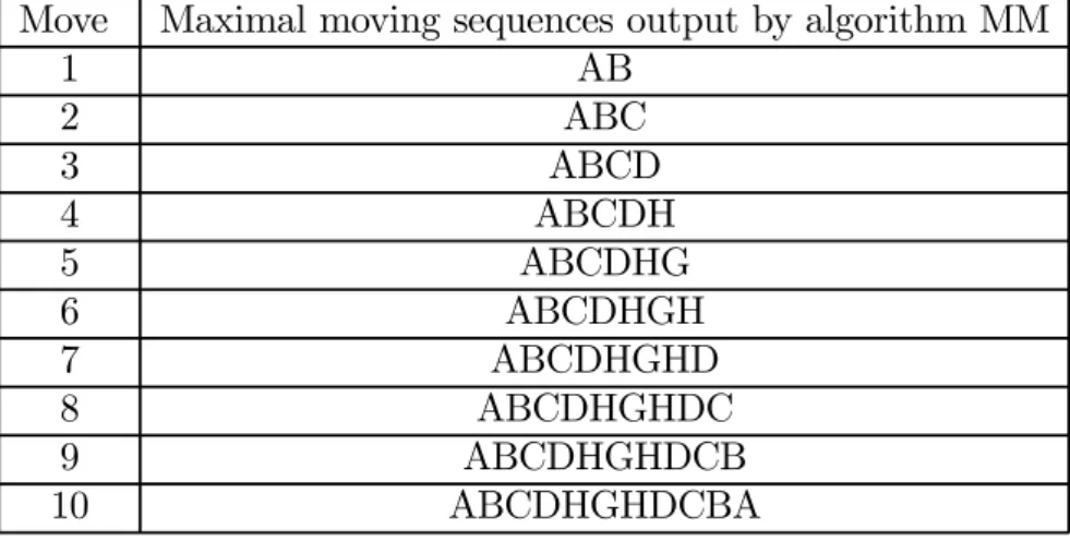
Move Maximal moving sequences output by algorithm MM 1 AB 2 ABC 3 ABCD 4 ABCDH 5 ABCDHG 6 ABCDHGH 7 ABCDHGHD 8 ABCDHGHDC 9 ABCDHGHDCB 10 ABCDHGHDCBA
Table 2.1: An illustrative example for algorithm MM
sequence), whose algorithmic form is given below, is applied to moving sequences of each mobile user to determine the maximal moving sequences of that user and update the occurrence count of moving pairs during registration procedure.
In algorithm MM, we use F to indicate if a node is revisited and Y to keep the current maximal moving sequence. DF denotes the database to store all the resulting maximal moving
sequences. S is the home location site of a mobile user. By the roundtrip model considered [10][17], the selection of S is either VLR or HLR whose geography area contains the homes of mobile users. Algorithm MM outputs a maximal moving sequence to DF until the S is reached.
In algorithm MM, moving sequences are scanned in line 2. A maximal moving sequence is output and a new maximal moving sequence will be explored (from line 14 to line 18) if MM finds that Ni in the moving pair (Oi, Ni) is the same as the starting site S. Otherwise, Ni is appended into
Y (in line 12) and the occurrence count of (Oi,Ni) is updated on-line in the database (in line 14).
An example execution scenario by algorithm MM is given in Table 2.1 Algorithm MM /* Algorithm MM for finding maximal moving sequences */ Input: A moving sequence {((O , N ), (O , N ), ...(O , N )} of a mobile user.
Output: Maximal moving sequences of the mobile user. begin
1. Set i to 1 and string Y to null , where Y is used to keep the current maximal moving sequence and S is the starting point.
2. while (not end of movings) 3. begin 4. Set A = Oi and B = Ni; 5. if (A == S ) 6. begin 7. Set Y=S; 8. Append B to Y; 9. end 10. else 11. begin 12. Append B to string Y ;
13. Update the occurrence count of (A,B) in database DF;
14. if (B == S ) 15. begin
16. Output string Y to database DF;
17. Set Y to null; 18. end 19. end 20. i++; 21. end end
2.2.2
Finding Large Moving Sequences
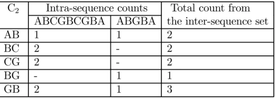
As long as we obtain the maximal moving sequences, the large moving sequences are next to be determined. A large moving sequence can be determined from all maximal moving sequences of each individual user based on its occurrences in those maximal moving sequences. We define intra-sequence count to be the number of occurrences of a moving sequence within a maximal moving sequence, and inter-sequence set of a moving sequence to be the set of maximal moving sequences which contain that moving sequence. The count of a large moving sequence is the sum of intra-sequence counts from its inter-sequence set. For the example in Table 2.2, the
intra-sequence count of GB in {ABCGBCGBA} is 2 and that in {ABGBA} is 1. Also, the inter-sequence set of GB is {{ABCGBCGBA}, {ABGBA}}. Hence, the count of GB is the sum of intra-sequence counts in its inter-sequence set (i.e. 2 ( i.e., intra-sequence count in ABCGBCGBA) +1 (i.e., intra-sequence count in ABGBA)=3). Algorithm LM (standing for large moving sequence) is then developed for the determination of large moving sequences. Let Lk represent the set of all large k-moving sequences and Ck be a set of candidate k-moving
sequences.
Algorithm LM /* Algorithm for finding large moving sequences */ Input: A set of w maximal moving sequences of a mobile user. Output: Large moving sequences of the mobile user.
begin
1. Determining L2= {large 2-moving sequence} from moving pairs in C2;
2. for (k = 3; Lk−16= 0, k + +) 3. begin
4. Ck= Lk−1∗ Lk−1;/* Generating Ck from Lk−1∗ Lk−1 */
5. for w maximal moving sequence S 6. begin
/* Calculating the intra-sequence count of Ck within S */
7. intra-sequence =sub-sequence(Ck, S);
8. if (intra-sequence>0)
9. Including S into inter-sequence set;
/* sum of occurrence counts in a inter-sequence set */ 10. for all candidate c ∈ inter-sequence
11. c.count=c.count+c.intra-sequence; 12. end
13. Lk= {c ∈ Ck | c.count>support };
14. end end
As pointed out in [14], the initial candidate set generation, especially for L2, is the key issue
to improve the performance of data mining. Since occurrence counts of moving pairs, i.e., C2,
were updated on-line in the data collection phase, L2 can be determined by proper trimming on
C2 Intra-sequence counts Total count from
ABCGBCGBA ABGBA the inter-sequence set
AB 1 1 2
BC 2 - 2
CG 2 - 2
BG - 1 1
GB 2 1 3
Table 2.2: An example for counting the occurrences of 2-moving sequences
note that Ck can be simply generated from Lk−1∗ Lk−1(line 4). For example, with the set of L2
being {AB, BK}, we have a C3 as {ABK}. As explained above, the occurrence count of each
k-moving sequence is the sum of intra-sequence counts (from line 5 to line 9 in algorithm LM) in its inter-sequence set (i.e., line 10 and line 11 in algorithm LM). Note that this step is very different from that in mining the path traversal patterns [1] where there are no loops in a moving sequence (i.e., the corresponding intra-sequence count is always zero). The occurrences of each k-moving sequence in Ckare determined for the identification of Lk. After the summation of the occurrence
counts in the inter-sequence set from line 10 to line 11 in algorithm LM, those k-moving sequences with counts exceeding the support are qualified as Lk (line 13 of algorithm LM). Notice that those
large k-moving sequences are obtained from w maximal moving sequences of that mobile user, showing the incremental mining capability of algorithm LM. For illustrative purposes, with the maximal moving sequences of a mobile user being {ABCGBCGBA, ABGBA}, Table 2.2 shows the corresponding counts of C2.
As mentioned above, the main drawback of [15] is the generation of moving log for all mobile users. In practice, generating the moving log of all mobile users unavoidably leads to the increased storage cost and degraded performance of mobile computing systems. In order to reduce the effort
of generating moving log, we explore regression for mining user moving patterns from the existing log of call detail records (referred to as CDR).
Chapter 3
Mining User Moving Patterns
3.1
Preliminary
In this paper, assume that the moving behavior of mobile users have periodicity and consecutive movements of mobile users are not too far. Therefore, if the time interval of two consecutive CDRs is not too large, the mobile user is likely to move nearby. Two location models (i.e., geometric model and symbolic model) are available for the location identification techniques [2]. In geometric model, the location is specified as n-dimensional coordinates (typically n=2 or 3). For example, the location pair returned by global positioning system at time t is expressed by (Xt, Yt) where Xt is the value of location in horizontal coordinate axis, whereas Yt is the
corresponding value of location in vertical coordinate axis. In symbolic model, the system uses logical entities to describe the location spaces. For example, in mobile computing systems, the base station identification is used to represent the location of mobile users. In our prior work [15], user moving patterns are represented in symbolic model (i.e., base station identification). In this
paper, we will take both two location models into consideration. To facilitate the presentation of this paper, a moving section is defined as a basic time unit. A moving record is a data structure that is able to accumulate the counting of base station identifications (henceforth referred to as item) appearing in call detail records whose occurring time are within the same moving section. Given a log of call detail records, we will first convert these CDR data into multiple moving sequences where a moving sequence is an ordered list of moving records and the length of the moving sequence is ε. The value of ε depends on the periodicity of mobile users and is able to obtain by proposed method in [6]. As a result, a moving sequence i is denoted by <M R1i, M R2i, M R3i, ..., M Riε>, where M R
j
i is the jth moving record of moving sequence
i. Assume the basic unit of a moving section is four hours and the value of ε is six. Given the log data in Table 1.1, we have the moving sequence M S1 = < {A : 1}, {}, {D : 1}, {}, {},
{G : 1, I : 1} >. Time projection sequence of moving sequence MSiis denoted as T PM Si,which is
formulated as T PM Si = < α1, ..., αn>, where M R
αj
i 6= {} and α1 < ... < αn.Explicitly, T PM Si is
a sequence of numbers that are the identifications of moving sections in which the corresponding moving records are not empty. Given M S1 =< {A : 1}, {}, {D : 1}, {}, {}, {G : 1, I : 1} >,
one can verify that T PMS1 =< 1, 3, 6 >. By utilizing the technique of sequential clustering,
a time projection sequence T PM Si is able to divide into several groups in which time intervals
among moving sections are close. For the brevity purpose, a clustered time projection sequence of T PM Si, denoted by CT P (T PM Si) is represented as < CL1, CL2, ..., CLx > where CLi is the
3.2
Procedure for Mining User Moving Patterns
In Section 3.1, we develop a solution procedure, which is composed of a sequence of algorithms in the corresponding phases, to mine approximate user moving patterns. Specifically, with the multiple moving sequences converted from the log of call detail records, we develop algorithm LS to identify those moving sequences beneficial to discover approximate user moving patterns in Section 3.2. Then, in Section 3.3, by exploring the spatial-temporal locality, we devise algorithm TC to cluster call detail records in time projection sequences. In Section 3.4, a regression-based algorithm MF is devised to mine approximate user moving patterns.
3.2.1
An Overview
The overall procedure for mining moving patterns is outlined as follows: Procedure for Mining Approximate User Moving Patterns
Step 1. (Data Collection Phase) Employing algorithm LS to mine the regularity of moving sequences from original call detail records for every w moving sequence, where w is an adjustable window size for recent moving sequences to be considered.
Step 2. (Time Clustering Phase)Employing algorithm TC to cluster call detail records into groups and then generate a clustered time projection sequence.
Step 3. (Regression Phase) Employing algorithm MF to derive moving functions of mobile users from a clustered time projection sequence.
As mentioned before, once the log of call detail records is given, we shall covert the log data into multiple moving sequences, each of which is an ordered list of moving records. Generally speaking, call detail records not only contain the regularity of user moving behaviors but also
have noise data accidentally generated. For example, a mobile user has some call detail records during his vacation. These call detail records are viewed as noise data in this paper. As mentioned before, we explore the technique of regression analysis, which is very sensitive to noise data, to derive moving functions for mobile users. Thus, in data collection phase, algorithm LS is able to determine similar moving behaviors of mobile users for every w moving sequences. By exploring the feature of spatial-temporal locality, which refer to the feature that if the time interval between two consecutive calls of a mobile user is small, the mobile user is likely to move nearby, algorithm TC is employed to cluster call detailed records with spatial-temporal locality into several groups. After obtaining the clustering groups, we develop algorithm MF that takes both temporal and spatial data of similar moving records into consideration to determine approximate user moving patterns. The details of mining algorithms are described in the following subsections.
3.2.2
Data Collection Phase
As mentioned early, in this phase, we shall identify similar moving sequences from a set of w moving sequences obtained and then merge these similar moving sequences into one aggregate moving sequence (to be referred to as AM S). Algorithm LS is applied to moving sequences of each mobile user to determine the aggregate moving sequence that contains a sequence of large moving records denoted as LM Ri, where i = [1, ε]. Specifically, large moving record LM Rj is a
set of items with their corresponding counting values if there are a sufficient number of M Rji of moving sequences containing these items. Such a threshold number is called vertical_min_sup in this paper. Once the aggregate moving sequence is generated from these recent w moving sequences, we will then compare this aggregate moving sequence with these w moving sequences
so as to further accumulate the occurring counts of items appearing in each large moving record. The threshold to identify the similarity between moving sequences and the aggregate moving sequence is named by match_min_sup. The algorithmic form is given below.
Algorithm LS
input: w moving sequences with their length being ε,
two threshold:vertical_min_sup and match_min_sup output: Aggregate moving sequence AM S
1 begin 2 forj =1 to ε 3 for i=1 to w 4 LM Rj =large 1-itemset of M Rij; (by vertical_min_sup) 5 fori =1 to w 6 begin 7 match = 0; 8 forj = 1 to ε 9 begin 10 C(M Rji, LM Rj) = |x ∈ MRji ∩ LMRj| / |y ∈ MR j i ∪ LMRj|; 11 match = match+|MRji|*C(MRij, LM Rj); 12 end
13 if match≥ match_min_sup then 14 accumulate the occurring counts of
items in the aggregate moving sequence; 15 end
16 end
In algorithm LS (from line 2 to line 4), we first calculate the appearing count of items in each moving sections of w moving sequences. If the count of an item among w moving sequence is larger than the value of vertical_min_sup, this item will be weaved into the corresponding large moving record. After obtaining all large moving records, AM S is then generated and is represented as < LM R1, LM R2, ...LM Rε>,where the length of given moving sequence is ε. As mentioned before, large moving records contains frequent items with their corresponding counts. Once obtaining the aggregate moving sequence, we should in algorithm LS (from line 5 to line 12) compare this aggregate moving sequence with w moving sequences in order to identify those
similar moving sequences and then calculate the counts of each item in large moving records. Note that a moving sequence (respectively, AM S) consists of a sequence of moving records (respectively, large moving records). Thus, in order to quantity how similar between a moving sequence (e.g., M Si) and AM S, we shall first measure the closeness between moving record
M Rji and LM Rj, denoted by C(M Rj i, LM Rj). C(M R j i, LM Rj)is formulated as |{x∈MRji∩LMRj}| |{y∈MRij∪LMRj}|
that returns the normalized value in [0, 1]. The larger the value of C(M Rji, LM Rj) is, the more
closely M Rji resembles LM Rj. For example, we set large moving records LM Rj =
{a, b, c, d}, M Rj
x = {b, e} and MRjy ={a, b, c, d, e}. It can be verified that the value of C(MRjx, LM Rj) is 1
5 and the value of C(M R j
y, LM Rj) is 45. Clearly, M R j
y is more similar to LM Rj than M Rjx is.
Accordingly, the similarity measure of moving sequence M Siand AM S is thus able to formulated
as sim(M Si, AM S) =Pεi=1|MRji|∗C(MR j
i, LM Rj).Given a threshold value match_min_sup,
for each moving sequence M Si, if sim(M Si, AM S)≥ match_min_sup, moving sequence MSi
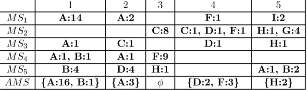
is identified as a similar moving sequence. In algorithm LS (from line 13 to line 14), for each item in large moving records, the occurring count is accumulated from the corresponding moving records of those similar moving sequences. Given an illustrative example in Table 3.1, we have sim(M S1, AM S) = 1∗12+1∗11+0+1∗12+1∗01 = 2. Consequently, we also have sim(M S2, AM S) =
3, sim(M S3, AM S) = 2, sim(M S4, AM S) = 3, and sim(M S5, AM S) = 12. Assume that
match_min_sup is 2. Compared with AM S, M S1, M S2, M S3 and M S4 are then recognized
as similar moving sequences. After identifying those similar moving sequences, algorithm LS is able to calculate the occurring count of each item in large moving records. Consider LM R1 of
AMS in Table 2 as an example. From those similar moving sequences, the occurring count of A in LM R1 is calculated as the sum of the count of A in M R1
1 2 3 4 5
M S1 A:14 A:2 F:1 I:2
M S2 C:8 C:1, D:1, F:1 H:1, G:4
M S3 A:1 C:1 D:1 H:1
M S4 A:1, B:1 A:1 F:9
M S5 B:4 D:4 H:1 A:1, B:2
AM S {A:16, B:1} {A:3} φ {D:2, F:3} {H:2}
Table 3.1: An example of algorithm LS
(i.e., 14 + 1 + 1 = 16). Following the same procedure, we could have AM S <{A : 16, B : 1}, {A : 3}, φ, {D : 2, F : 3}, {H : 2}> shown in Table 3.1.
It can be verified that algorithm LS is of polynomial time complexity. With w moving sequences and the length of a moving sequence being ε, the complexity of algorithm LS can be expressed by O(εω). Specifically, the complexity of calculating large moving records is O(εω) and that of extracting regular moving sequences is ε ∗ ω ∗ O(1) = O(εω). As a result, the overall time complexity of algorithm LS is O(εω).
3.2.3
Time Clustering Phase
Recall that the time projection sequence of moving sequence M Si is denoted as T PMSi, which
is presented as T PM Si =< α1, ..., αn >, where M R
αj
i 6= {} and α1 < ... < αn. Once obtaining
AM S, we could easily determine T PAM S. By exploring the feature of spatial-temporal locality,
we will in this phase develop algorithm TC to generate a clustered time projection sequence of AM S (i.e., CT P (T PAM S)).
In algorithm TC, two threshold values (i.e., δ and σ2) are given in clustering a time projection
make sure that the spread of the time is bounded within σ2. Algorithm TC is able to dynamically
determine the number of groups in a time projection sequence. Algorithm TC
input: Time projection sequence T PAM S,
threshold δ and σ2
output: Clustered time projection sequence CT P (T PAM S)
1 begin
2 group the numbers whose differences are within δ; 3 mark all clusters;
4 while there exist marked clusters and δ >= 1 5 foreach marked clusters CLi
6 if V ar(CLi)≤ σ2
7 unmark CLi;
8 δ = δ− 1;
9 forall marked clusters CLi
10 group the numbers whose differences are within δ in CLi;
11 end while
12 if there exist marked clusters 13 for each marked cluster CLi
14 k = 1; 15 repeat 16 k++;
17 divide evenly CLi into k groups ;
18 until the spread degree of each group≤ σ2;
19 end
By grouping those numbers together if the difference between two successive numbers is smaller than the threshold value δ, algorithm TC (from line 2 to line 3) first starts coarsely clustering T PAM Sinto several marked clusters. As pointed out before, CLidenotes the ith marked
cluster. In order to make sure that quality of clusters, variance of CLi, denoted as V ar(CLi),
is defined to measure the distribution of numbers in cluster CLi. Specifically, V ar(CLi) is the
variance of a sequence of numbers. Hence, V ar(CLi) is formulated as m1 m P k=1 (nk− m1 m P j=1 nj)2,
line 5 to line 7 in algorithm TC, for each cluster CLi, if V ar(CLi)is smaller than σ2, we unmark
the cluster CLi. Otherwise, we will decrease δ by 1 and with given the value of δ, algorithm TC
(from line 8 to line 10) will re-cluster those numbers in unmark clusters. Algorithm TC partitions the numbers of T PAM S iteratively with the objective of satisfying two threshold values, i.e., δ
and σ2, until there is no marked cluster or δ = 0. If there is no marked clusters, CT P (T P
AM S)is
thus generated. Note that, however, if there are still marked clusters with their variance values larger than σ2, algorithm TC (from line 12 to line 18) will further finely partition these marked
clusters so that the variance for every marked cluster is constrained by the threshold value of σ2.
If the threshold value of δ is 1, a marked cluster is usually a sequence of consecutive numbers in which the variance of this marked cluster is still larger than σ2. To deal with this problem, we
derive the following lemma:
Lemma 1: Given a sequence of consecutive integers Sn with the length being n, the variance of
Sn is 121(n2 − 1).
Proof:
Note that the variance of the sequence of consecutive integers with the same length is the same. For example, consider two sequences of consecutive integers: {1, 2, 3, 4, 5} and {7, 8, 9, 10, 11}. It can be verified that V ar({1, 2, 3, 4, 5}) = V ar({7, 8, 9, 10, 11}). Without loss of generality, consider the variance V ar({1, 2, 3, ..., n}).
Let ¯x is the average of {1, 2, ...n}, ¯x = (n(n+1)2 )/n = n(n+1)2n = 1+n2 . Then V ar({1, 2, 3, ..., n}) = n1( n P x=1 (x− ¯x)2) = n1( n P x=1 x2− 2¯x n P x=1 x + ¯x n P x=1 1) = (n+1)(2n+1)6 − (n + 1)¯x + ¯x2
= (n+1)(2n+1)6 − (n+1)2 2 + (n+1 2 ) 2 = (n+1)(2n+1)6 − (n+1)4 2 = 121 (n + 1)(4n + 2− 3n − 3) = 1 12(n + 1)(n− 1) = 121 (n2 − 1) ¤
Property: Given a sequence of consecutive integers {1, 2, 3, ..., n} and a positive integer k, the optimal way of dividing {1, 2, 3, ..., n} into k clusters is to partition {1, 2, 3, .., n} into k clusters with each cluster size being dnke.
Proof:
Suppose {1, 2, 3, ..., n} is divided into {1, ..., t1}{t1+ 1, ..., t2}, ..., {tk−1+ 1, ..., n}.
Let t0 = 1, tk = n, and V ari = V ar({ti−1, ti−1+ 1, ..., ti}). Our goal is to find the point t1,
t2, ..., and tk−1with the purpose of minimizing f = k
P
i=1
V ari.
From lemma 1, V ar({1, 2, ..., n}) = 121(n 2 − 1), we have f = k P i=1 V ari = 121 k P i=1 ((ti− ti−1)2− 1). To minimize f = k P i=1
V ari, the cutting points t1, t2, ..., and tk−1 are derived by letting first
derivatives be zero.⎧ ⎪ ⎪ ⎪ ⎪ ⎪ ⎪ ⎪ ⎪ ⎪ ⎪ ⎨ ⎪ ⎪ ⎪ ⎪ ⎪ ⎪ ⎪ ⎪ ⎪ ⎪ ⎩ ∂f ∂t1 = 4t1− 2t2− 2t0 = 0 ∂f ∂t2 = 4t2− 2t3− 2t1 = 0 ... ∂f ∂tk−1 = 4tk−1− 2tk− 2tk−2 = 0
⎧ ⎪ ⎪ ⎪ ⎪ ⎪ ⎪ ⎪ ⎪ ⎪ ⎪ ⎨ ⎪ ⎪ ⎪ ⎪ ⎪ ⎪ ⎪ ⎪ ⎪ ⎪ ⎩ t1 = ti02+t2 t2 = t1+t2 3 ... tk−1 = tk−2+tk 2
By using substitution method, we could have ⎧ ⎪ ⎪ ⎪ ⎪ ⎪ ⎪ ⎪ ⎪ ⎪ ⎪ ⎨ ⎪ ⎪ ⎪ ⎪ ⎪ ⎪ ⎪ ⎪ ⎪ ⎪ ⎩ t1 = 12t2 t2 = 23t3 ... tk−1 = k−1 k tk
Therefore, we can get: ⎧ ⎪ ⎪ ⎪ ⎪ ⎪ ⎪ ⎪ ⎪ ⎪ ⎪ ⎨ ⎪ ⎪ ⎪ ⎪ ⎪ ⎪ ⎪ ⎪ ⎪ ⎪ ⎩ t1 = 1kn t2 = 2kn ... tk−1 = k−1k n
From the derivation above, the optimal way to divide {1, 2, 3, ..., n} into k clusters is to divide {1, 2, 3, .., n} into k clusters with each cluster size being dnke.
By the above property, given marked cluster CLi,algorithm TC initially sets k to be 1. Then,
marked cluster CLi is evenly divided into k groups with each group size dnke. By increasing the
value of k each run, algorithm TC is able to partition the marked cluster until the variance of each partition in the marked cluster CLi satisfies σ2.
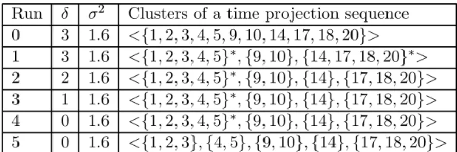
Consider the execution scenario in Table 3.2 where the time projection sequence is T PAM S
= <1, 2, 3, 4, 5, 9, 10, 14, 17, 18, 20>. Given σ2 = 1.6 and δ = 3, algorithm TC first roughly
Run δ σ2 Clusters of a time projection sequence 0 3 1.6 <{1, 2, 3, 4, 5, 9, 10, 14, 17, 18, 20}> 1 3 1.6 <{1, 2, 3, 4, 5}∗, {9, 10}, {14, 17, 18, 20}∗> 2 2 1.6 <{1, 2, 3, 4, 5}∗, {9, 10}, {14}, {17, 18, 20}> 3 1 1.6 <{1, 2, 3, 4, 5}∗, {9, 10}, {14}, {17, 18, 20}> 4 0 1.6 <{1, 2, 3, 4, 5}∗, {9, 10}, {14}, {17, 18, 20}> 5 0 1.6 <{1, 2, 3}, {4, 5}, {9, 10}, {14}, {17, 18, 20}>
Table 3.2: An execution scenario under algorithm TC.
(i.e., {1, 2, 3, 4, 5} with V ar({1, 2, 3, 4, 5})=2 and {14, 17, 18, 20} with V ar({14, 17, 18, 20})=4.69) are determined due to that the variance values of these two clusters are larger than 1.6. Then, δ is reduced to 2, and these two marked clusters are examined again. Following the same procedure, algorithm TC partitions mark clusters until δ equals 1. As can been seen in Run 4 of Table 3.2, {1, 2, 3, 4, 5} is still a marked cluster with V ar({1, 2, 3, 4, 5})=2. Therefore, algorithm TC finely partitions {1, 2, 3, 4, 5}. The value of k is initially set to be 1. Since V ar({1, 2, 3, 4, 5})=2.5 is larger than σ2
(i.e., 1.6), k is increased to 2. Then, {1, 2, 3, 4, 5} is divided into {1, 2, 3}{4, 5}. Among these two clusters (i.e., {1, 2, 3} and {4, 5}), {1, 2, 3} has the larger variance and thus {1, 2, 3} is compared with the value of σ2. Note that since the variance of {1, 2, 3} = 0.67 < 1.6, algorithm TC stops clustering. After the execution of algorithm TC, a CT P (T PAM S)is generated
as <{1, 2, 3}, {4, 5}, {9, 10}, {14}, {17, 18, 20}>.
The time complexity of algorithm TC is of polynomial time complexity. Explicitly, let T PAM S
have n numbers. In line 2 of algorithm TC, we have O(n) to roughly divide sequence into t the clusters. Note that from line 4 to line 11 of algorithm TC, we have O(δmt) to group the original sequence. From 13 to 19, assume that there are still t clusters with m numbers to be refined and then we have t ∗ m ∗ (m) = O(m2t) to run the clustering process. Since algorithm TC is a
heuristic algorithm, we consider the worst case when estimating the time complexity of algorithm TC. Assume that the worst case is that t = m = n, and thus the overall time complexity of algorithm TC is at most O(n3).
3.2.4
Regression Phase
Given aggregate moving sequence AM S devised by algorithm LS with its clustered time projec-tion sequence CT P ( T PAM S) generated by algorithm TC, in this phase, algorithm MF is able
to derive a sequence of moving functions that are able to estimate moving behaviors of mobile users.
Assume that AM S is <LM R1, LM R2, ..., LM Rε>with its clustered time projection sequence CT P (T PAM S) = < CL1, CL2, ..., CLk>, where CLi represents the ith cluster. For each cluster
CLiof CT P ( T PAM S), we will derive the estimated moving function of mobile users, expressed as
Ei(t) = ( ˆxi(t), ˆyi(t), valid_time_interval ), where ˆxi(t)(respectively, ˆyi(t)) is a moving function
in x-coordinate axis (respectively, in y-coordinate axis)) and the moving function is valid for the time interval indicated in valid_time_interval.
Without loss of generality, let CLi be {t1, t2, ..., tn} where ti is one of the moving section in
CLi. As described before, a moving record has the set of the items with their corresponding
counts. Therefore, we could extract those large moving records from AM S to derive the estimated moving function for each cluster. In order to derive moving functions, the location of base stations should be represented in geometry model through a map table provided by tele-companies. Hence, given AM S and a cluster of CT P (T PAM S), for each cluster of CT P (T PAM S), we could
represent as (t1,x1,y1,w1), (t2,x2,y2,w2), ...(tn,xn,yn,wn). Accordingly, for each cluster of CT P (
T PAM S), regression analysis is able to derive the corresponding estimated moving function. By
exploring the technique of regression analysis, the moving functions devised are able to generate the curves close to the data points and thus can be used to estimate users’ moving behaviors.
The regression analysis fits equations of approximating curves to the raw field data [23]. For a given set of data, the fitting curves are generally not unique. Note that a curve with a minimal deviation from all data points is desired. Let ei be the error between the ith data point and the
estimated fitting curve. Given a set of data points, the best estimated curve is the one that has the minimal sum of least square errors (i.e., the minimal value of x, where x =
Pn
i=1e
2 i) [23].
Since the number of calls may be varied for each distinct (ti, xi, yi), it is reasonable to derive
moving functions by taking the weights into consideration. Therefore, the regression analysis with weighted least squares is then applied.
Given a cluster of data points (e.g., (t1, x1, y1, w1), (t2, x2, y2, w2), ..., (tn,xn,yn,wn)), we
first consider the derivation of ˆx(t).An m-degree polynomial function ˆx(t) = a0+ a1t + ... + amtm
will be derived to approximate moving behaviors in x-coordinate axis. Specifically, the regression coefficients {α0, α1, ...am} are chosen to make the residual sum of squares x =
Pn
i=1wie2i minimal,
where wi is the weight of the data point (xi, yi)and ei = (xi−(a0+a1ti+a2(ti)2...+am(ti)m)).The
value of m is determined in accordance with the requirement of applications but m is usually smaller than the number of data points. To facilitate the presentation of our paper, we define the following terms:
H= ⎡ ⎢ ⎢ ⎢ ⎢ ⎢ ⎢ ⎢ ⎢ ⎢ ⎢ ⎣ 1 t1 (t1) 2 ... (t1)m 1 t2 (t2)2 ... (t2)m ... ... ... ... ... 1 tn (tn) 2 ... (tn)m ⎤ ⎥ ⎥ ⎥ ⎥ ⎥ ⎥ ⎥ ⎥ ⎥ ⎥ ⎦ , a∗ = ⎡ ⎢ ⎢ ⎢ ⎢ ⎢ ⎢ ⎢ ⎢ ⎢ ⎢ ⎣ a0 a1 ... am ⎤ ⎥ ⎥ ⎥ ⎥ ⎥ ⎥ ⎥ ⎥ ⎥ ⎥ ⎦ , ˜bx = ⎡ ⎢ ⎢ ⎢ ⎢ ⎢ ⎢ ⎢ ⎢ ⎢ ⎢ ⎣ x1 x2 ... xn ⎤ ⎥ ⎥ ⎥ ⎥ ⎥ ⎥ ⎥ ⎥ ⎥ ⎥ ⎦ , e = ⎡ ⎢ ⎢ ⎢ ⎢ ⎢ ⎢ ⎢ ⎢ ⎢ ⎢ ⎣ e1 e2 ... en ⎤ ⎥ ⎥ ⎥ ⎥ ⎥ ⎥ ⎥ ⎥ ⎥ ⎥ ⎦ T , W = ⎡ ⎢ ⎢ ⎢ ⎢ ⎢ ⎢ ⎢ ⎢ ⎢ ⎢ ⎣ w1 w2 ... wn ⎤ ⎥ ⎥ ⎥ ⎥ ⎥ ⎥ ⎥ ⎥ ⎥ ⎥ ⎦ .
It can be verified that the residual sum of squares (i.e., x =Pni=1wie2i) can be expressed as x = eTWein linear algebra manner. Note that e is able to be formulated as ( ˜bx− Ha∗).Thus,
we have: x = eTWe = (˜bx− Ha∗)TW(˜bx− Ha∗) = (˜bx− Ha∗)T √ W√W(˜bx− Ha∗) 1 = (√W˜bx− √ WHa∗)T(√W˜b x− √ WHa∗) =||√W˜bx− √ WHa∗||
let A = √WH and B = √W˜bx. It can be seen that the main objective is to minimize x = ||B − Aa∗||. According to the theorem of least squares, B − Aa∗ must be orthogonal to
Aa∗ so as to minimize x[8]. For interest of brevity, the theorem of least squares is omitted in
this paper. Consequently, we can have: B− Aa∗ ∈ R(A)⊥ = N (AT)
, where R(A)⊥ represents the orthogonal complement of column space of A and N (AT) represents the kernel space of AT
=⇒ AT(B
− Aa∗) = 0 =⇒ ATAa∗ = ATB
ATAa∗ = ATB is viewed as the normal equation [8]. By substituting A = √WH and B = √W˜bx, we could have (
√
WH)T(√WH)a∗ = (√WH)T√W˜b
x. By solving the normal
equation, we can a∗ such that the value of
x is minimized. Therefore, ˆx(t) = a0+ a1t + ... + amtm
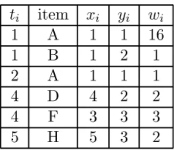
ti item xi yi wi 1 A 1 1 16 1 B 1 2 1 2 A 1 1 1 4 D 4 2 2 4 F 3 3 3 5 H 5 3 2
Table 3.3: Data points with their corresponding weights.
is obtained. Following the same procedure, we could derive ˆy(t). As a result, for each cluster of CT P (T PAM S), the estimated moving function Ei(t) = (ˆx(t), ˆy(t), [t1, tn]) of a mobile user is
devised.
Consider an illustrative example in Table 3.1, where AM S = <{A : 16, B : 1}, {A : 3}, φ, {D : 2, F : 3}, {H : 2}>. Assume that CT P (T PAM S) =< {1, 2, 4, 5} > and the coordinates of
A, B, D, F and H are (1, 1), (1, 2), (4, 2), (3, 3) and (5,3), respectively. Given AM S and CT P (T PAM S) =< {1, 2, 4, 5} >, we could have the data points with their weights shown in
Table 3.3. By choosing m to be 3, the 3-degree polynomial ˆx(t) = a0 + a1t + a2t2 + a3t3
is derived. Due to that the coefficients a0, a1, a2 and a3 are unknown, we intend to have
a regression curve with the purpose of minimizing the residual sum error. In other words, a∗ = ( a
0 a1 a2 a3 )
T should be determined. Since there are five data points with their
corresponding moving sections are 1, 2, 4, 4 and 5, H = ⎡ ⎢ ⎢ ⎢ ⎢ ⎢ ⎢ ⎢ ⎢ ⎢ ⎢ ⎢ ⎢ ⎢ ⎢ ⎣ 1 1 (1)2 (1)3 1 2 (2)2 (2)3 1 4 (4)2 (4)3 1 4 (4)2 (4)3 1 5 (5)2 (5)3 ⎤ ⎥ ⎥ ⎥ ⎥ ⎥ ⎥ ⎥ ⎥ ⎥ ⎥ ⎥ ⎥ ⎥ ⎥ ⎦ is then obtained.
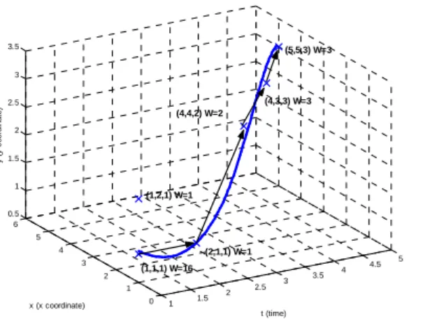
1 1.5 2 2.5 3 3.5 4 4.5 5 0 1 2 3 4 5 6 0.5 1 1.5 2 2.5 3 3.5 t (time) x (x coordinate) y ( y c o or dina te ) (1,1,1) W=16 (1,2,1) W=1 (2,1,1) W=1 (4,4,2) W=2 (4,3,3) W=3 (5,5,3) W=3
Figure 3.1: An illustrative example, where the arrow line is the real moving path and the solid line is estimated by moving functions obtained by algorithm MF.
sum of 16 and 1. The weights of data points are 17, 1, 2, 3 and 2, respectively. Hence, √W is a diagonal matrix with its diagonal entries to be [√17,√1,√2,√3,√2].From Table 3.3, we can get ˜
bx = ( 1 1 4 3 5 )T. By solving the equation (
√ WH)T(√WH)a∗ = (√WH)T√W˜b x, we can get a∗ = ( 2.333 −2.133 0.867 −0.066 )T. Therefore ˆx(t) = 2.333 −2.133t+0.867t2 − 0.066t3is devised to predict the x coordinate-axis of the mobile user from t = 1 to t = 5. Similarly, ˜
by = ( 1 2 1 2 3 3 )T is then determined from Table 3.3. By solving the normal equation
(√WH)T(√WH)a∗ = (√WH)T√W˜b
y, we can get a∗ = ( 2.529 −2.386 1.021 −0.105 )T.
Consequently, ˆy(t) = 2.529−2.386t+1.021t2−0.105t3is obtained. The estimated moving function is shown in Figure 3.1. It can be seen that the estimated moving function is very close to the real moving path, showing the advantage of utilizing regression in mining user moving patterns. Algorithm MF
input: AM S and clustered time projection sequence CT P (T PAM S)
output: A set of moving functions
F (t) ={E1(t), U1(t), E2(t), ..., Ek(t), Uk(t)}
2 initialize F (t)=empty; 3 for i= 1 to k-1 4 begin
5 doing regression on CLi to generate Ei(t);
6 doing regression on CLi+1 to generate Ei+1(t);
7 t1 =the last number in CLi;
8 t2 =the first number in CLi+1;
9 using inner interpolation to generate Ui(t) = (ˆxi(t), ˆyi(t), (t1, t2));
10 insert Ei(t), Ui(t) and Ei+1(t)in F (t);
11 end 12 if(1 /∈ CL1)
13 generate U0(t) and Insert U0(t) into the head of F (t);
14 if(ε /∈ CLk)
15 generate Uk(t) and Insert Uk(t) into the tail of F (t);
16 return F (t); 17 end
Given AM S and a cluster of CT P (T PAM S) = <CL1, CL2, ..., CLk>, algorithm MF is able
to generate the whole estimated moving function, denoted as F (t). F (t) is represented as {U0(t),
E1(t), U1(t), E2(t), ..., Ek(t), Uk(t)}, where Ei(t) is the estimated moving function in cluster
i of CT P (T PAM S) and Ui(t) is the linkage moving function from Ei(t) to Ei+1(t). It is shown
in algorithm MF (from line 5 to line 6) that for each cluster of CT P (T PAM S), we could
de-rive the corresponding estimated moving functions by the regression method mentioned above. Note that, however, it is possible that the first moving section is not in CL1. If t0 is the first
number of CL1 and t0 6= 1, the U0(t) = {E1(t0), [1, t0)} is generated for the boundary
condi-tion. Otherwise, U0(t) will not be valid in F (t). The situation of Uk(t) is similar. The linkage
moving function will be calculated by interpolation (in line 9 of algorithm MF). For example, assume that CT P (T PAM S)=<{1, 2, 4, 5}{7, 9, 10}>, E1(t)=(2.333 − 2.133t + 0.867t2− 0.066t3,
2.529−2.386t+1.021t2−0.105t3, [1, 5])and E2(t) = (10−2.17t+0.17t2, 32−6.33t+0.33t2, [7, 10]).
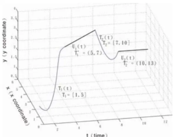
Figure 3.2: A snapshot of complete moving function F (t)
The last number of {1, 2, 4, 5} is 5 and the first number of cluster {7, 9, 10} is 7. Thus, a linkage moving function should be generated by inner interpolation. From E1(t),at time 5, we can have
a data point (x = 5.09, y = 3). At time 7, a data point ( x = 3.14, y = 3.86 ) is generated by applying E2(7). By inner interpolation, we could have U1(t) = (9.965 + 3.14−5.097−5 t, 0.85 + 3.86−37−5 t,
(5,7)). Similarly, U2(t)can be produced. Thus, we could have F (t) = {E1(t), U1(t), E2(t), U2(t)}.
The snapshot of F(t) is shown in Figure 3.2.
When using F (t) to predict the location of a mobile user, we will only use the estimated moving function whose time interval includes the given time t. For the above example F (t) = {E1(t), U1(t), E2(t), U2(t)}, given the time to be 4, only E1(t)will be used to predict the location
since the given time 4 is within the time interval of E1(t). Once the estimated moving function is
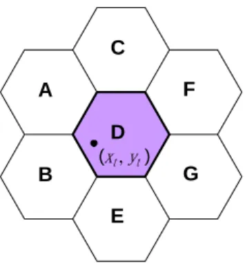
obtained, it is straightforward to generate the approximate moving patterns in symbolic model. By utilizing the estimated moving function derived, the location of a mobile user is predicted as (xt, yt).Since each base station is aware of its location and converge area, as shown in Figure 3.3,
(xt ,yt) A B C D E F G
Figure 3.3: An illustrative example for transformation from geometric model to symbolic model Note that the time complexity of algorithm MF is of polynomial time complexity. Specifi-cally, with the maximal size in row/column being n, the time complexity of solving the normal equation by Strassen’s algorithm is Θ(nlg 7) [19]. Moreover, the interpolation by Lagrange’s for-mula requires Θ(m2), where m represents the number of points involved in the interpolation [19].
Since n is usually larger than m, the value of Θ(nlg 7) is the dominating factor of the complexity
Chapter 4
Performance Study
In this section, the effectiveness of mining approximate user moving patterns by call detail records is evaluated empirically. The simulation model for the mobile system considered is described in Section 4.1. Section 4.2 is devoted to experimental results and comparison with the original algorithm of mining moving patterns [15]. Finally, sensitivity analysis of mining approximate user moving patterns is shown in Section 4.3.
4.1
Simulation Model for a Mobile System
To simulate base stations in a mobile computing system, we use an eight by eight mesh network, where each node represents one base station and there are hence 64 base stations in this model [13][15]. A moving path is a sequence of base stations travelled by a mobile user. The number of movements made by a mobile user during one moving section is modeled as a uniform distribution between mf -2 and mf +2. There are 10,000 users considered in our simulation model. According to Law of Large Number[23], we repeat each experiment for 20 times and every result presented
in the figures is the average performance of 20 experimental results. Explicitly, the larger the value of mf is, the more frequently a mobile user moves. To model user calling behavior, the calling frequency is employed to determine the number of calls during one moving section. If the value of cf is large, the number of calls for a mobile user will increase. Similar to [15], the mobile user moves to one of its neighboring base stations depending on a probabilistic model. To make sure the periodicity of moving behaviors, the probability that a mobile user moves to the base station where this user came from is modeled by Pback and the probability that the mobile
user routes to the other base stations is determined by (1-Pback)/(n-1) where n is the number of
possible base stations this mobile user can move to. We assign two Pback to each users to present
the major and minor moving behavior respectively. As mentioned before, the method of mining moving patterns in [15], denoted as U M P , is implemented for the comparison purposes. For interest of brevity, our proposed solution procedure of mining user moving patterns is expressed by AU M P (standing for approximate user moving patterns). The location is represented as the identifications of base stations. To measure the prediction accuracy, we use the hop count (denotes as hn), which is measured by the number of base stations, to represent the distance from the prediction location to the actual location of the mobile user. Intuitively, a smaller value of hn implies that the more accurate prediction is achieved. It is worth mentioning that the expected value of hop count per call, denoted by E(hn/call), is w∗ε∗cf/2hn where cf /2 is the expected value of the number of CDR in a time unit. Thus a precise ratio is defined as 1 −E(hn/call)−12n . Precise
ratio is a measurement considering not only the distance between the moving patterns and real paths but also the ratio of the distance and the whole network size. Table 4.1 summarizes the definitions for some primary simulation parameters and the measurements of performance.
Notation Definition Value
w retrospective factor various value used M s the number of moving sections in a moving sequence various value used M f moving frequency various value used Cf call frequency various value used σ2 variance threshold various value used
vertical_min_sup threshold of vertical minimal support various value used match_min_sup threshold of match minimal support various value used
Table 4.1: The parameters and measurements used in the simulation
0.7 0.75 0.8 0.85 0.9 0.95 1 3 5 7 9 11 13 15 17 19 moving frequency pr eci se r at io UMP AUMP
Figure 4.1: The precise ratio of UMP and AUMP with the value of mf varied.
4.2
Experiments of UMP and AUMP
To conduct the experiments to evaluate U M P and AU M P , we set the value of w to be 10, the value of cf to be 3 and the value of ε to be 12. The precise ratio of U M P and AU M P with various values of mf are shown in Figure 4.1. It can be seen that by having a moving log, which contains the entire moving behaviors of users, the precise ratio of U M P is higher than that of AU M P.
As mentioned before, U M P is able to mine user moving patterns from a set of moving log in which every movement of mobile user is recorded. Note, however, that though performing
0 0.05 0.1 0.15 0.2 0.25 3 5 7 9 11 13 15 17 19 moving frequency co st r at io UMP AUMP
Figure 4.2: The cost ratios of AUMP and UMP with the moving frequency varied
better than AU M P in the hop count, U M P incurs more amount of data in the moving log. In order to reduce the amount of data used in mining user moving patterns, AU M P explores the log of call detail records. The cost ratio for a user, i.e., amount of log dataprecise ratio , means the prediction accuracy gained by having the additional amount of log data. Figure 4.2 shows the cost ratios of U M P and AU M P . Notice that AU M P has larger cost ratios than U M P , showing that AU M P employs the amount of log data more cost-efficiently to increase the prediction accuracy.
4.3
Sensitivity Analysis of AUMP
The impact of varying the values of w for mining approximate moving patterns is next investi-gated. Without loss of generality, we set the value of ε to be 12, that of mf to be 3, and the values of cf to be 1, 3 and 5. Both vertical_min_sup and match_min_sup are set to 20% , the value of δ is set to be 3 , and σ2 is set to be 0.25. With this setting, the experimental results
are shown in Figure 4.3.
60% 65% 70% 75% 80% 85% 90% 95% 100% 5 10 15 20 25 30 restropective factor pr ec is e rat io users with cf=1 users with cf=3 users with cf=5
Figure 4.3: The performance of AUMP with the value of w varied.
0.83 0.85 0.87 0.89 0.91 0.93 0.95 5% 10% 15% 20% 25% vertical_min_sup pr ecis e ra tio
AUMP with match_min_sup=10% AUMP with match_min_sup=20% AUMP with match_min_sup=30%
Figure 4.4: The precise ratio of AUMP with vertical_min_sup and match_min_sup varied. sequences considered in AUMP increases, AUMP is able to effectively extract more information from the log of call detail records. Note that with a given the value of w, the precise ratio of AUMP with a larger value of cf is bigger, showing that the log of data has more information when the value of cf increases. Clearly, for mobile users having high call frequencies, the value of w is able to set smaller in order to quickly obtain moving patterns. However, for mobile users having low call frequencies, the value of w should be set larger so as to increase the accuracy of moving patterns mined by AU M P .
0.7 0.75 0.8 0.85 0.9 0.95 1 0.1 0.25 0.75 1 1.5 2 variance threshold pr ec is e ra ti o
A U M P w ith m atch_m in_sup=10% A U M P w ith m atch_m in_sup=20% A U M P w ith m atch_m in_sup=30%
Figure 4.5: The precise ratio of AUMP with the values of match_min_sup and the variance threshold varied.
Now, the experiments of varying the values of vertical_min_sup and match_min_sup for algorithm LS are conducted where we set the value of cf to be 5, that of mf to be 1, that of ε to be 12 and that of σ2 to be 0.25. The precise ratio of AU M P with various values of
vertical_min_sup and match_min_sup are shown in Figure 4.4, where it can be seen that the precise ratio of AU M P with a given vertical_min_sup tends to increase as the value of match_min_sup increases. The reason is that increasing the match_min_sup is able to efficiently filter out call detail records that are viewed as noise data. As such, the precision of AU M P with higher match_min_sup is larger. In addition, with a given match_min_sup, the precise ratio of AU M P increases, as the value of vertical_min_sup increases. This is due to that as the value of vertical_min_sup increases, the more frequent set of base stations is determined from a set of call detail records. Thus, the frequent set of base stations, referring to areas that users more frequently travel, are very helpful to approximate user moving patterns.
As described before, the value of σ2 for algorithm TC affects the precision of time clustering