利用快速傅立葉轉換增加蒙地卡羅評價衍生性金融商品的效率

國 立 交 通 大 學

應用數學系

碩 士 論 文

利用快速傅立葉轉換增加蒙地卡羅方法評價衍生性

金融商品的效率

Efficient Valuation of Financial Derivatives by

Monte Carlo Simulations with Fast Fourier

Transform

研 究 生：尤頌文

指導老師：王克陸 教授

許元春 教授

利用快速傅立葉轉換增加蒙地卡羅方法評價衍生性

金融商品的效率

Efficient Valuation of Financial Derivatives by

Monte Carlo Simulations with Fast Fourier

Transform

研 究 生: 尤頌文 Student：Sung-Wen Yu

指導教授: 王克陸 Advisor：Keh-Leh Wang

許元春 Yuan-Chung Sheu

國 立 交 通 大 學

應 用 數 學 系

碩 士 論 文

Submitted to Department of Applied Mathematics College of Science

National Chiao Tung University in Partial Fulfillment of the Requirements

for the Degree of Master

in

Applied Mathematics June 2007

Hsinchu, Taiwan, Republic of China

利用快速傅立葉轉換增加蒙地卡羅方法評價衍生性

金融商品的效率

學生: 尤頌文

指導教授: 王克陸 教授 & 許元春 教授

國立交通大學應用數學系(研究所)碩士班

摘 要

在本篇文章中，我們提出了使用快速傅立葉演算法來加速

蒙地卡羅評價選擇權的方法。我們以快速傅立葉演算法計算選

擇權的Delta值，並且利用這些Delta值去建立馬丁格爾控制變

異數項來降低估計值的變異數。我們發現結合快速傅立葉演算

法與馬丁格爾控制變異數方法在增加運算效率方面是非常有

用的，並且也保留了運算的正確性。同時我們也討論了利用快

速傅立葉演算法的誤差分析。

Efficient Valuation of Financial Derivatives by

Monte Carlo Simulations with Fast Fourier

Transform

Student：Sung-Wen Yu

Advisor：Keh-Leh Wang & Yuan-Chung Sheu

Department (Institute) of Applied Mathematics

National Chiao Tung University

ABSTRACT

In this paper, we proposed the use of Fast Fourier transform (FFT) method

to accelerate Monte Carlo simulations in option pricing. The method of FFT is

applied to compute the Deltas of the options. These Deltas are essential in

construct martingale control for variance reduction. We find that the

combination of the FFT method with the martingale control variate method is

very useful to reduce the computational time while preserving the accuracy of

simulations. The error analysis of using FFT method is also discussed.

誌 謝

這篇論文的完成，首先要感謝我的指導老師 王克陸教授以

及給我在寫論文期間很多很多指導的清大 韓傳祥教授。 謝謝王

老師在財務知識方面給我很多的指導，更感謝韓老師在寫論文迷

惘期間給我一盞明燈，讓我找到方向，獻上最誠懇的感謝。口試

期間，也承蒙韓傳祥老師、張焯然老師費心審閱並提供了寶貴的

意見，使得本論文得以更加的完備，永誌於心。

在這兩年求學的過程中，要感謝非常多人，在研一時，發覺

自己對數學理論沒有特別興趣，想改走財金路線。謝謝 許元春

老師在研一的時候給了我ㄧ個良好的建議，也同意我去找財金所

的 王克陸老師，讓我得以在此領域發展，使我的人生有了轉變，

非常感謝這兩位老師。

除此之外，也要感謝我研究所的同學和學弟和數學系的系羽

同伴們，謝謝他們肯陪我打羽毛球，讓我得以再苦澀的研究生活

中找到一個發洩的管道，同時也要感謝十一舍 403 的室友們，高

方、國忠和彥維陪我一起摩獸爭霸與魔獸世界，讓我度過無聊的

時光，也讓我擁有這些美好的回憶。

最後，要感謝我的父母在背後默默的支持，讓我得以放心的

讀書做研究。願與所有關心我的人一起分享這份喜悅，再次地感

謝所有幫助過我及關心過我的人，謝謝大家！

目

錄

中文提要

………

i

英文提要

………

ii

誌謝

………

iii

目錄

………

iv

一、

Introduction ………

1

二、

2.1

2.2

Hedging Martingale Control with Variance Reduction..

Review of Martingale Control Variate Method

………

Example

………

3

3

7

三、

3.1

3.2

3.3

3.4

四、

4.1

4.2

4.3

4.3.1

4.3.2

4.4

4.5

五、

5.1

5.1.1

5.2

5.2.1

六、

Apply FFT Method to Price Option

………

Introduction of FFT

………

Fourier Transform Of Option Price

………

Evaluation of Option Price by FFT Method………….

Example………

Delta Estimation Using FFT Option Pricing Method…

Introduction………..

Examples………..

Error of Using FFT Option Pricing Method To

Estimate Delta………

Truncation Error………

Sampling Error………..

Apply FFT Option Pricing Method in Martingale

Control Variate Method………

Numerical Result………..

More Examples……….

Stochastic Volatility Model: Heston Model………….

Numerical Result………..

American Option………..

Numerical Result………..

Conclusion………

8

9

9

14

15

18

18

22

26

26

28

30

32

35

35

37

38

40

41

七、

A

B

C

Appendix

………

Proof Claim 9 in Section 3.1

………

Algorithm of FFT(Fast Fourier Transform)

………

Derivation of the accuracy of the variance analysis…

43

43

44

47

References

………

50

1

Introduction

The method of Monte Carlo simulations is a very popular technique which is applied in many scholastic …elds, such as physics, engineering, statistics, …nance, and so on. This method is based on the analogy between proba-bility and volume. The measure theory formalizes the intuitive notion of probability of the event to be its volume or measure relatives to that of a universe of possible outcomes. Monte Carlo uses this identity in reverse, to calculate the volume of a set by interpreting it as a probability. For example, we can randomly sample from a universe of possible outcomes and take the fraction of random draws that fall in a given set as an estimate of the set’s volume. According to the law of large numbers, this estimate converges to the correct value as the number of draws increases. The advantage of Monte Carlo simulations is that it is no or less sensitive to dimensionality of the un-derlying problem and suitable for parallel computations. However the main disadvantage of this method is that the rate of convergence is slow because it is limited by the central limit theorem. It is relatively slow compared to deterministic schemes for low dimensional problems.

To improve the e¢ ciency of Monte Carlo methods, there are two main possible approaches : Quasi Monte Carlo simulation (QMC) and variance reduction technique. Quasi Monte Carlo simulations are also called low-discrepancy methods. The main di¤erence between QMC and the Monte

Carlo method is that QMC makes no attempt to mimic the underlying ran-domness. Indeed, it seeks to increase the accuracy speci…cally by generating points evenly to obtain the randomness. QMC forms a class of methods where low-discrepancy numbers are generated in a deterministic way while basic Monte Carlo uses pseudo-random numbers. Variance reduction method exploits information about the errors to reduce the errors in estimates of un-known variables. On the other hand, this method seeks probabilistic ways to reformulate the undertaken problem in order to gain signi…cant variance reduction. For example, control variate methods take into account the corre-lation properties of random variables, but the e¢ ciency of these techniques is often restricted to certain undertaken problems.

In …nancial applications such as pricing derivatives, taking the control as a (local) martingale is a very useful method. This method is called “martin-gale control variate method.”The martin“martin-gale control variate method can be well understood in …nance terminology. The constructed control variate cor-responds to a continuous Delta hedge strategy taken by a trader who sells an option. So this method is also known as “hedging martingale variance control method”. Fouque and Han [7] apply this method to price European option, American option, and Barrier option(down and out) in stochastic volatility models. Also they show the variance analysis of this method. However, the weakness of this method is that it takes time to compute the parameter val-ues for each path. If we want to estimate an option price by Monte Carlo simulations, we will construct many simulated paths. The martingale con-trol is a stochastic integral consisting of a partial derivative, known as Delta. We need to compute Delta at each simulated time step. Section 2 will de-scribe the martingale control variate method in detail. The purpose of this paper is to apply the fast Fourier transform (FFT) methodology to reduce

FFT option pricing method is …rst developed by Carr and Madan [14]. They use Fourier transform to change the option pricing problem from the real domain to the complex domain. This Fourier transform can be repre-sented by the characteristic function of the natural logarithm of the under-lying at the expiration date. The reason for using characteristic function is that under some models or processes, the characteristic functions are eas-ier to compute. For example, under Levy processes, we can have general forms of characteristic functions. See, Bertoin [6] in detail. We can take inverse Fourier transform to get the option price. FFT is used to approx-imate this inverse Fourier transform. In other words, this method requires only the characteristic function of the natural logarithm of the underlying at maturity. Borak, Detlefsen, and Härdle [21] use this method to price call op-tion under Heston model and Bates model. Itkin [2] applies this in variance gamma (VG) process. Lee [15] o¤ers the error bound of this method. The restriction of this method is it is only suitable for pricing European option. Based on this method, we estimate the Delta in the related Black-Scholes model. Moreover, we give the error analysis of this estimation.

The rest of this paper is arranged as the following. In section 2, we review the martingale control variate method, and discuss its computational issue of this method. Section 3 introduces the FFT option pricing method and discusses the models which can apply this method. In section 4, we apply FFT option pricing method to compute the Delta of the call option in geometric Brownian motion (GBM) environment using martingale control variate method, and illustrate numerical results in …gures. Moreover, the error bound of this method is computed. Finally, we conclude in section 5.

2

Hedging Martingale Control with Variance

Reduction

2.1

Review of Martingale Control Variate Method

Under the risk-neutral probability space ( ; F; (Ft)0 t<1; P ), we consider

the risky underlying asset St which is governed by the geometric Brownian

motion

dSt = rStdt + StdWt, (1)

where r is a risk-free rate and is the volatility. Both r and are constants. W_t is the Brownian motion under risk-neutral probability. There are two corollaries of this model.

Corollary 1 The logarithm of the underlying asset St follows the normal

distribution with mean (r 1₂ 2_{)t and variance} 2_{t. i.e.}

log St N ((r

1 2

2_)t; 2_{t) (2)}

Corollary 2 The closed form solution of this model is ST = Stexp((r

1 2

2_{)(T t) + W}

T t), (3)

where St is the price of the underlying asset at time t.

Given this model, the fair price of a European-style derivative with ma-turity T < 1, denoted by P , is simply a conditional expectation

where Et;x denotes the expectation with respect to P conditioned on the

current states St = x, H(x) the payo¤ function satisfying the integrability

condition. For example, H(x) = maxfx K; 0_{g for strike price K > 0,} it is a call payo¤. A‘…nancial contract with the call or put payo¤ is called a European call option or a European put option respectively. From the simulation point of view, it is straightforward to construct the basic Monte Carlo estimator of the option price P (0; S0) at time 0 by

1 Q Q X i=1 e rTH(S_T(i)), (5) where Q is the total number of independent sample paths and S_T(i) denotes the i-th independent replication of the underlying asset price at time T:

Assuming that the European option price P (t; x) is smooth enough, we apply Ito’s lemma to its discounted price e rtP, and then integrate from time 0to the maturity T . The following martingale representation is obtained

P (t; x) = e rTH(ST) M0(P ; T ) (6)

where centered martingale is de…ned by M0(P ; T ) =

Z T o

e rs@P

@x(s; Ss) SsdWs. (7) Remark 3 M0(P ) is a martingale and it has mean zero.

This martingale plays the role of “perfect” control for Monte Carlo sim-ulations and the integrand consists of the perfect Delta hedge if the partial derivative @P_@x(t; x) is known so that the option price P (t; x) would be known in advance. In reality, P (t; x) is not known. Therefore, equation (6) is not feasible for a direct computation for the option price. Nevertheless by em-ploying a martingale as a control we can formula the unbiased control variate estimator 1 Q Q X i=1 [e rTH(S_T(i)) M₀(i)(PBS; T )] (8)

for the option price P0 = E [e rTH(ST) M0(PBS; T )jF0] where the

mar-tingale control M0(PBS; T ) consists of the price approximation PBS of the

actual option price P . That is M0(PBS; T ) =

Z T o

e rs@PBS

@x (s; Ss) SsdWs, (9) where PBS is the solution of Black-Scholes partial di¤erential equation with

the terminal condition PBS(T; x) = H(x). In …nancial interpretation M0(PBS; T )

represents the Delta hedging portfolio accumulated up to time T, so the term M0(PBS; T )is called the hedging martingale be the price PBS so that the

esti-mator de…ned by (9) is called the martingale control variate estiesti-mator. Apply Ito’s isometry, the variance of the controlled payo¤ P0 is simply the sum of

quadratic variations of martingale :

V ar(e rTH(ST) M0(PBS; T )) (10) = E_0;xf Z T o e 2rs(@P @x(s; Ss) @PBS @x (s; Ss)) 2 2_S2 sds.g.

Therefore, if the Delta trading @PBS

@x (t; x) is closed to the actual hedging

strategy, the variance of the martingale control estimator should be small. Now, we introduce the algorithm to estimate the martingale control.

Step1. Simulate the underlying asset’s paths in order to obtain the terminal prices of the asset. Compute the sample paths of H(ST) and its discounted

value e rT _H(S

T).

Step2. Discretize the martingale control of the e rT _H(S

T). Use the lower

Riemann sum to approximate the integral (9) . i.e. M0(PBS; T ) = Z T o e rs@PBS @x (s; Ss) SsdWs (11) M X @P T rT

where f0;MT ; T

M 2; :::; T

M (M 1)g is the partition of the interval [0; T ] ,

K is the strike price of option, and "j are identical and independent (I.I.D)

standard normal random variables.

Step3. An estimator of the martingale control variate for the option price is the following, E_0;x[e rTH(ST) Z T o e rs@PBS @x (s; Ss) SsdWs] (12) 1 Q( Q X l=1 e rTH(S_T(l)) Q X l=1 M X j=1 e rMT(j 1)@PBS @x ( T M(j 1); S (l) T M(j 1) ) S(l)T M(j 1) r T M"j, where Q is the number of sample paths.

2.2

Examples

We take two examples in European call option to observe the e¢ ciency of the martingale control variance method. The payo¤ function H(x) = (x K)+, where K is the strike price. We suppose the risk-free rate r = 0:1 , the volatility = 0:25, and the maturity T = 1. The current time is assumed 0, and the initial underlying asset price S0 is 100. In the …rst example, we take

the strike price K as 80 to …t the case of in-the-money. The other example, we take K = 120 which is in the out-of-the money environment. Let the number of sample paths Q = 10000 and the partitions of time interval [0; T ] = 100. We compare the standard error (SE) of Monte Carlo simulations with and without martingale control. We also show the CPU time spending in these two conditions. The variance reduction ratio is also represented.

(1) K = 80

Call Price Standard Error Time(Seconds) Using martingale control variate 28.581 0.0107 63.5897

The variance reduction ratio =590:83 (2) K = 120

Call Price Standard Error Time(Seconds) Using martingale control variate 6.638 0.0195 65.7116

Without using martingale control variate 6.589 0.1407 0.4317 The variance reduction ratio =52:062

From numerically results, we can observe that when we use martingale control variate to reduce variance, the standard error is diminished so much. As we know, the convergence rate of Monte Carlo simulations is governed by 1=pQ, where Q is the number of sample paths. In the …rst example, if we want to reduce the standard error from the method of without using martingale control variate to that of using martingale control variate, the sample paths should be increased from 10000 to 6250000 approximately. This is the power of the martingale control variate method. But there comes a disadvantage of this method, it spends a lot of time. The time using martingale control variate method is much greater that it without using this method. Observe the martingale control in equation (9), we can …nd that the most part of time spending in martingale control variate method is to compute the term @PBS

@x (t; x), which is call the Delta of the option.

We would estimate Delta values @PBS

@x (t; x) in every pairs (t; St), where t 2

f0;MT ; T

M 2; :::; T

M (M 1)g. For this reason, we want to search some methods

to increase the e¢ ciency in computing martingale control. We …nd that take advantage of FFT option pricing method to compute Delta may be a feasible way. Next, we introduce the FFT option pricing method and explain how to use this method to make the martingale control variate method more e¢ ciently.

3

Apply FFT Method to Price Option

In this section, we will introduce how to apply Fast Fourier transform (FFT) method to price the call option. The approach has been addressed by Carr and Madan [14]. The big attraction of this method is the Fast Fourier trans-form (FFT) could be used to make computation more e¢ cient. This e¢ ciency is even boosted by the possibility of the pricing algorithm to calculate prices for a whole range of strikes. The other advantage for this method is that if we know the characteristic function of nature logarithm of underlying asset price at maturity, this method can be applied directly. The characteris-tic function often has a simple form for many models while the probability density functions of the log price is often not get in the closed form.

3.1

Introduction of FFT

FFT is …rst developed by Cooley and Tukey [8]. It is an e¢ cient algorithm for computing the summation

w(k) =

N

X

j=1

e i2N(j 1)(k 1)x(j) for k = 1,. . . ,N , (13)

where N is typically a power of 2. The power of FFT is that the method can compute the element of the sequence fw(1); w(2),...,w(N)g rapidly. The algorithm reduces the number of multiplications in the require N summations from an order of N2 _{to that of N log}

2N, a very considerable reduction. We

go into details this algorithm in appendix B.

3.2

Fourier Transform of Option Price

We de…ne some notations and these notations are used around this section. Let CT(k) be the discounted value of the call option with maturity T at the

current time 0. k is the natural logarithm of the strike price K of the option. And we use St to represent the underlying asset price at time t. The initial

price of asset is denoted by S0. In this method, we usually suppose S0 = 1

for convenience. We also de…ne XT = log ST.

De…nition 4 The characteristic function of the natural logarithm of the price of the underlying asset , XT, is de…ned by

T(u), E [exp(iuXT)] =

Z 1 1

eiusqT(s)ds (14)

where qT(s) is the probability density function of XT under the risk-neutral

world.

De…nition 5 De…ne AXT as the set

AXT , fv 2 R

n_{: E [e}u XT_{] <}

1g; (15) where is the inner product.

De…nition 6 De…ne XT as the set

XT , f 2 C

n

: Im( )_{2 A}XTg , (16)

the complex vectors whose negated imaginary parts are in XT form a “strip”or

“tube”.

Lemma 7 The characteristic function T is well-de…ned and analytic

(in…-nitely di¤erentiable) in X, which is a convex set. Partial derivative of T

De…ne the initial (discounted) call value CT(k) is related to the

risk-neutral density qT(s) by:

C0;T(k; S0) , E [e rT(max(eXT ek; 0))] = Z 1 1 e rT max(es ek; 0)qT(s)ds = Z ₁ k e rT(es ek)qT(s)ds:

Here, simply, we suppose the risk-free rate, r is a constant.

Theorem 8 For any p > 0, C0;T(k; S0) e rTE [exp(p + 1)XT] (p + 1) exp(pk) ( p p + 1) p _{and C} 0;T(k; S0) e rTE [exp XT] (17)

Proof. For all s 0 we have

s ek s p+1 (p + 1) exp(pk)( p p + 1) p ,

because the left-hand and right-hand sides, as function of s, have equal values and …rst derivatives at s = (p + 1)exp(k)=p, and the second derivative of the right-hand side is always positive. Moreover, since the right-hand side is positive, the left side can improve to (s exp(k))+_{:Now, substitute s =}

exp(XT), take expectations, and discount both sides to obtain the …rst bound.

The second bound is obvious.

De…nition 9 _{The Fourier transform of the function f on R is de…ned by} '(v) =

Z

R

f (x)eivxdv (18) and its attached inversion is given by

f (x) = 1 2

Z

R

Lemma 10 _{The Fourier transform of the function f on R exists if kfk1}is …nite or f 2 L1(R). i.e. _Z

R

jf(x)j dx < 1. (20)

Lemma 11 _{If f 2 L}1_{(R), then lim}

x! 1f (x) = 0:

But, we know that when k = logK tends to negative in…nity, in other words, the strike price K tends to zero, the option is deeply in the money, and the discounted option price tends to the initial underlying price. That is

lim

k! 1C0;T(k; S0) = S0 6= 0: (21)

By the lemma 11 , we know that the Fourier transform of the discounted call option price does not exist. To make C0;T(k; S0) to be an absolutely

integral function, we add a parameter into C0;T(k; S0), the parameter is

usually called the “damping parameter”. Consider the modi…ed call price de…ned by

c0;T(k; S0), exp( k)CT(k) (22)

for > 0. [The reason for > 0is that we want c0;T(k; S0)tends to zero as k

tends to negative in…nity. For a range of positive value of , we expect that c0;T(k; S0)is integrable in k over the entire real line. How to choose the value

of will be discussed later. Consider the Fourier transform of c0;T(k; S0), X(T )

T (v) =

Z

R

eivkc0;T(k; S0)dk. (23)

Lemma 12 We develop an analytical expression for X(T )_T (v) in terms of

T(v). i.e. X(T ) T (v) = e rT T(v ( + 1)i) 2_{+ v}2_{+ i(2 + 1)v}. (24)

Proof. X(T ) T (v) = Z R c0;T(k; S0)eivkdk = Z ₁ 1 eivk Z ₁ k e ke rT(es ek)qT(s)dsdk = Z 1 1 e rTqT(s) Z s 1 e k(es ek)eivkdkds = Z 1 1 e rTqT(s) Z s 1 es+ k+ivk ek+ k+ivk dkds = Z 1 1 e rTqT(s) es+ k+ivk + iv ek+ k+ivk + 1 + iv s 1 ds = Z 1 1 e rTqT(s) es+ s+ivs + iv es+ s+ivs + 1 + iv ds = Z 1 1 e rTqT(s) es+ s+ivs ( + iv)( + 1 + iv)ds = e rT ( + iv)( + 1 + iv) Z ₁ 1 qT(s)es+ s+ivsds = e rT ( + iv)( + 1 + iv) Z 1 1

qT(s)ei(v (( +1)i))sds

= e

rT

T(v ( + 1)i) 2_{+ v}2_{+ i(2 + 1)v}

Then, we take the inverse Fourier transform of T(v) and undamp it to

get the call price,

C0;T(k; S0) = e k 1 2 Z 1 1 X(T ) T (v)e ivk_{dv. (25)}

Lemma 13 The call option price can be simpli…ed to the following form C0;T(k; S0) = e k

1 Z 1

0

Re( X(T )_T (v)e ivk)dv. (26)

Proof. See appendix A.

We note that the integration (26) is a direct Fourier transform and lends itself to an application of the FFT. Also note that in the denominator of (24) vanishes when v = 0, this is another reason for using damping parameter or

something similar is required. Positive value of assist the integrability of the modi…ed call value (22) over the negative nature logarithm of strike price axis, but aggravate the same condition for positive nature logarithm of strike price axis. For the modi…ed call value c0;T(k; S0) to be integrable in the

positive nature logarithm of strike price direction, a su¢ cient condition is provided by X(T )_T (0)being …nite. From (24), we observe that T( ( + 1)i)

should be …nite. It means that

( + 1) ₂ XT (27)

is a su¢ cient condition. Carr and Madan [14] proposed that one fourth of the upper bound which satisfying the condition (27) serves as good choice for . Schoutens [17] found that 0:75 is a good choice for and led to stable algorithms.

3.3

Evaluation of Option Price by FFT Method

The remainder work is to estimate the integral (26) numerically. Using the Trapezoid rule for the integral on the right-hand side of (26) and setting vj = (j 1), an approximation for CT(k) is:

C0;T(k; S0) t exp( k) Re( N X j=1 (e ivjk T(v) ): (28)

The e¤ective upper limit for the integration is now

U = N . (29)

value CT(k), which correspond to k near 0. The FFT returns N values of k

and we employ a regular spacing of size , so that our values for k are ku = b + (u 1), for u = 1,. . . ,N . (30)

This gives us log strike levels ranging from b to b where b = N

2 . (31) On the other hand, the sequence of strike price K correspond to ku is

K =_{fexp( b); exp( b + ); :::; exp( b + (N} 1))_g. (32)

Substituting (30) into (28) yields: CT(ku) t exp( ku) Re( N X j=1 (e ivj( b+ (u 1)) T(vj) ); for u = 1; : : : ; N . (33) Noting that vj = (j 1)and after arranging the summation, we get

CT(ku) t exp( ku) Re( N X j=1 (e i (j 1)(u 1)eibvj T(vj) ). (34)

Taking = 2_N, then the summation (34) becomes that CT(ku) t exp( ku) Re( N X j=1 (e i2N(j 1)(u 1)eibvj T(vj) ). (35)

Then the equation (35) …ts the FFT form (13). FFT method can be applied to compute the summation (35). Note that if we want to use FFT option pricing to evaluate call option price, the condition is we should know

T(v). By (24), T(v) can be represented as the function of characteristic

function of nature logarithm of underlying asset price at maturity, T(u).

method. This is very powerful. In many models, T(u) can be computed

easily. Next , we o¤er characteristic functions, T(u), in some models. And

these models can directly apply FFT option pricing method to pricing Eu-ropean derivatives.

3.4

Examples

(1) Merton model:

The price of the underlying asset follows the dynamics dSt

St

= rdt + dWt+ dZt, (36)

where Zt is a compound Poisson process with a log-normal distribution of

jump sizes. The jumps follow a Poisson process Nt with intensity which

is independent of Wt. The log-jump sizes Yi N ( ; 2) are i.i.d random

variables with mean and variance 2, which are independent of both Nt

and Wt. The dynamics of asset price is then given by:

St = S0exp( Mt + Wt+ Nt X i=1 Yi), (37) where M _{= r} 2 _{(exp( +} 1 2

2_{) 1). The characteristic function of}

XT = log ST is T(u) = exp[T ( 2_u2 2 ) + i M_{u + (exp(} 2 u2 2 + i u 1)]. (38) (2) Heston model:

The price of the underlying asset follows the dynamics dSt St = rdt +pvtdW (1) t (39) dv = ( v )dt + pv dW(2),

where vt is another unobservable stochastic process and follows the square

root process. So, this model is a type of “stochastic volatility model”. And the two Brownian motions W_t(1) and W_t(2) are correlated with rate . i.e.

Cov(dW_t(1); dW_t(2)) = dt. (40) Parameter measures the speed of mean reversion, is the average level of volatility and is the volatility of volatility. In (40) the correlation is typically negative, which is known as the “leverage e¤ect”.For the natural logarithm price of the underlying asset Xt= log St, one obtains the equation:

dXt = (r

1

2vt)dt + p_v

tdWt(1). (41)

The characteristic function of XT = log ST is T(u) =

exp( T ( 2i u) + iuT r + iux0)

(cosh ₂T + i usinh ₂T)22 exp( (u 2 _{+ iu)v} 0 coth ₂T + i u), (42) where = p 2_(u2_{+ iu) + ( i u)}2_{, and x}

0 and v0 are the initial values

for the log-price process and volatility process, respectively. (4) Bates model:

The price of the underlying asset follows the dynamics dSt St = rdt +pvtdW (1) t + dZt (43) dvt = ( vt)dt + pvtdW (2) t Cov(dW_t(1); dW_t(2)) = dt. (44) As in (43) Zt is a compound Poisson process with intensity and

log-normal distribution of jump sizes independent of Wt(1)and W (2)

t . If J denotes

the jump size then log(1 + J ) N (log(1 + &) 1₂ 2; 2) for some &. Under the risk neutral probability one obtains the equation for the logarithm of the asset price: dXt= (r & 1 2vt)dt + p_v tdW (1) t + ~Zt, (45)

where ~Zt is a compound Poisson process with normal distribution of jump

magnitudes. Since the jumps are independent of the di¤usion part in (36), the characteristic function of XT = log ST is

T(u) = D T(u) J T(u), (46) where D T(u) =

exp( T ( 2i u) + iuT (r &) + iux0)

(cosh ₂T + i usinh ₂T)22 exp( (u 2_{+ iu)v} 0 coth ₂T + i u) (47) is the di¤usion part characteristic function and

J

T(u) = exp(T (exp(

2_u2

2 + i(ln(1 + &) 1 2

2_{)u) 1), (48)}

is the jump part characteristic function. (5) Variance Gamma (VG) process:

The VG process is obtained by evaluating arithmetic Brownian motion with drift and volatility at a random time given by a gamma process having a mean rate per unit time of 1 and the variance rate of . The resulting process Xt( ; ; v) is a pure jump process with two additional parameters

and v relative to the Black Scholes model, providing control over skewness an kurtosis respectively.See [3] in detail. The underlying asset follows the process

St= S0exp(rt + Xt( ; ; v) + !t) t > 0, (49)

where by setting ! = (1=v) log(1 v 2_{v=2), the mean rate of return on the}

asset equals the interest rate r. The characteristic function of XT = log ST

is

T(u) = exp(log(S0+ (r + !)T )(1 i vu + 2u2v=2)) T =v. (50)

op-method, since we know the characteristic function of log ST, we can apply

this method to pricing call option. This is the advantage of this method. Next, we will apply this method to estimate the Delta of the call option.

4

Delta Estimation Using FFT Option

Pric-ing Method

4.1

Introduction

In this subsection, we discuss how to use the FFT pricing option method to compute the Delta of the call option. We also suppose that the price of underlying asset follows the geometric Brownian motion which is described in section 2. We use the notation t(k) to represent the Delta of the call

option at the time t. Simply, we let the current time is 0. k is the natural logarithm of the strike price K. The de…nition of delta t(k) is

t(k) =

@Ct(t; St)

@St

, (51) where T is the maturity of the call option. We will deduce it to our wanted form which can apply FFT option pricing method. Note that

Ct(t; St) = e r(T t)E [(ST K)+jS0] = e r(T t)E [(ST K)+], (52)

where the E is the expectation under the risk-neutral probability P . Recall that the closed form solution of ST under geometric Brownian motion is

ST = Stexp((r

1 2

2_{)(T t) + W}

W_{T t}is the Brownian motion under risk-neutral probability with mean 0 and variance T t. Then substitute (3) and (2) into (1), we obtain that

t(k) = @e r(T t)_{E [(S} texp((r 1₂ 2)T + WT t) K)+] @St (54) = e r(T t)E [@(Stexp((r 1 2 2_{)(T t) + W} T t) K)+ @St ] (1) = e r(T t)E [I_{fST Kg}exp((r 1 2 2_{)(T t) + W} T t)]; (2)

where I_fST Kg is the indicator function. i.e.

I_{fST Kg} = 8 > < > : 1; if ST K 0; otherwise. .

In order to simplify t(k), we use the following lemma, called Girsanov’s

theorem.

Lemma 14 Let W (t), 0 t T, be a Brownian motion on a probability space ( ; F; P ), and let F (t), 0 t T, be a …ltration for this Brownian motion. Let (t), 0 t T , be an adapted process. De…ne

Z(t) = exp_f Z t 0 (u)dW (u) 1 2 Z t 0 2_(u)du g; ~ W (t) = W (t) + Z t 0 (u)du; and assume that

E[ Z T

0

2_(u)Z2_{(u)du] <}

1:

Set Z = Z(T ). Then E[Z] = 1 and under the probability measure ~

P (A) = Z

A

Z(w)dP (w) f or all A_{2 F;} the process ~W (t), 0 t T, is a Brownian motion.

In our case, we de…ne

and Z(t) = exp_f Z t 0 dW_u 1 2 Z t 0 2 du_{g = exp((} 1 2 2 )t + W_t); (56) then under the new probability measure

~ P (A) = Z A Z(w)dP (w) (57) ~

Wt is a Brownian motion. Then

t(k) = e r(T t)E [IxT Kg exp((r 1 2 2_{)(T t) + W} T t)] (58) = E[I~ _{f ~S} T Kg],

where log( ~ST) N ((r + 1₂ 2)(T t); 2(T t)). Let ~XT = log( ~ST), then t(k) could be rewrote as

t(k) = ~E[I_{f ~XT kg}] (59)

Now, we apply the FFT option pricing method to estimate this expec-tation. Note t(k) tends to 1 when k tends to 1, damping parameter

should be used to let t(k)2 L1(R). De…ne

~

t(k) = exp( k) t(k). (60)

The Fourier transform of ~t(k) is T(v) =

Z

R

eivk~t(k)dk. (61)

Lemma 15 We develop an analytical expression for T(v) in terms of the

characteristic function of ~XT, T(v). i.e. T(v) =

1

Proof. T(v) = Z R ~ t(k)eivkdk = Z ₁ 1 eivk Z ₁ k e kqT(s)dsdk = Z 1 1 qT(s) Z s 1 e keivkdkds = Z 1 1 ei(v i)s + iv qT(s)ds = 1 + iv T(v i),

where qT(s)is the density function of ~XT under the risk-neutral probability.

Lemma 16 If Y is a random variable whose probability density function follows the normal distribution with mean and variance 2_{, then the}

char-acteristic function of Y , '(t) is exp(i t 1 2 2 t2). (63) Proof. '(t) = Z R eiyt_p1 2 exp( (y )2 2 2 )dy = Z ₁ 1 1 p 2 exp( y2_{+ 2y} 2_{+ 2} 2_ity 2 2 )dy = Z 1 1 1 p 2 exp( (y ( + 2it))2 2 2 ) exp( 2 2it 4t2 2 2 )dy = exp(2 2_it 4_t2 2 2 ) Z 1 1 1 p 2 exp( (y ( + 2_it))2 2 2 )dy = exp( it 1 2 2 t2)

Since ~XT N ((r +1₂ 2)(T t); 2(T t)), by the above lemma, we obtain

Taking the inverse Fourier form of (61) and undamped, we obtain t(k) = exp( k) 1 2 Z R e ivk T(v)dv = exp( k) 1 Z 1 0 Re(e ivk T(v))dv. (65) Follow the FFT option pricing method, we transform t(k) into the FFT

form (13), t(ku) t exp( k) Re( N X j=1 (e ivj( b+ (u 1)) T(vj) ); for u = 1; : : : ; N , (66) the choice of b, , and k is the same as in FFT option pricing method in (29) (30) (31).

4.2

Examples

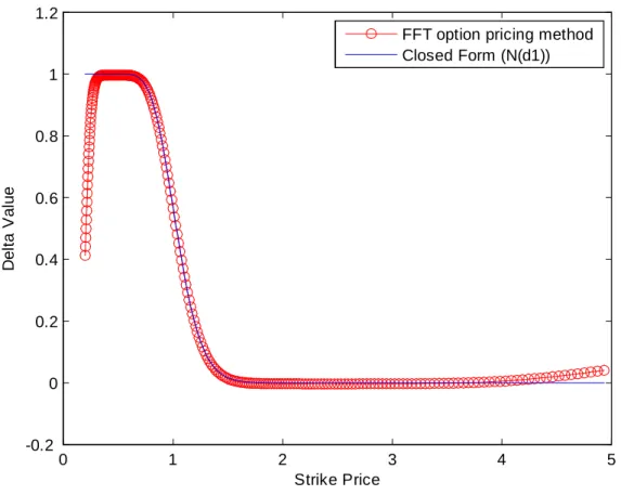
Now, we use this method to compute the Delta and compare the results of this method to the closed form solution.We choose N = 256, the truncated upper is 500, the damping parameter is 0:7, the risk-free rate r is 0:03, and volatility = 0:25. We compare two environments of maturity T = 0:5 and 1. In our setting, the sequence of natural logarithm of strike price

ku =f 64 125 ; 64 125 +250; 64 125 + 2 250; :::; 64 125 + 255 250g: We can …nd that in these two cases, the value of Delta is very near to the closed form solution when the strike price K is larger than 0.5. But when the strike price is smaller than 0.5, the method seems to be not suitable for estimating Delta. The reason may be the convergence rate of the FFT option pricing method is slow. If we focus on the at-the-money, out-the-money, even deeply out-the-money option, this method is good for computing Delta. In the next section, we will discuss the error of using FFT option pricing method to estimate Delta. We give the the upper bound of this error theoretically.

0 1 2 3 4 5 -0.2 0 0.2 0.4 0.6 0.8 1 1.2 Strike Price D el ta V al ue

FFT option pricing method Closed Form (N(d1))

Figure 1: Delta estimating using FFT option pricing method and closed form solution (T=0.5)

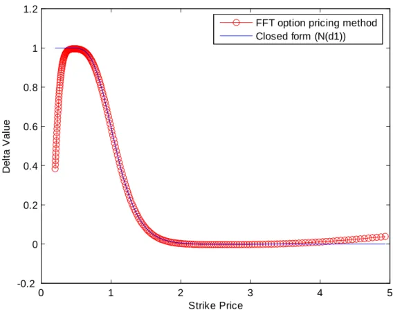
0 1 2 3 4 5 -0.2 0 0.2 0.4 0.6 0.8 1 1.2 Strike Price D e lta Va lu e

FFT option pricing method Closed form (N(d1))

Figure 2: Delta estimating using FFT option pricing method and closed form solution (T=1)

4.3

Error of Using FFT Option Pricing Method to

Es-timate Delta

The total error is de…ned as the absolute di¤erence between the true value

t(k) = exp( k)

Z 1 0

Re(e ivk T(v))dk,

and the discrete approximation given by the N -point sum X _N (k) = exp( k)Re( N X j=1 ( T(j ) exp( ij k) ).

The total error is bounded by the sum of the sampling error and the trunca-tion error t(k) X _N (k) t(k) X ₁ (k) + X 1(k) X N(k) , where P 1_{(k) is de…ned as} P N_{(k) is expect with an in…nite upper limit}

of summations. Truncation error because the upper limit of the numeric integration is …nite, and the sampling error because the integrand is evaluated numerically only at the grid points.

4.3.1 Truncation Error

Theorem 17 If _T is such that T(v) decays exponentially,j T(v)j (v) exp( v)

for all v U0, where > 0 and (v) is decreasing in v, then the truncation

error

X ₁

(k) X N(k) exp( k) (N ) exp( N )

1 exp( ) (67) provide that N > U0.

Proof. X ₁ (k) X N(k) exp( k) 1 X j=N j (vj) exp( vj)j exp( k) (N ) 1 X j=N exp( vj) exp( k)1 (N ) exp( N ) 1 exp( ) Note that by (40) and (42),

T(v) = exp((r + 1 2 2 )(T t)iv 1 2 2 (T t)v2), and T(v) = 1 + iv T(v i). Then j T(v)j T (v i) v = exp((r + 1 2

2_{)(T t)iv) exp(} 2_{(T t) i) exp((r +} 1 2 2_{)(T t) ))} v exp( 1₂ 2_{(T t)(v}2 2₎ v = exp((r + 1 2 2_{)(T t) ) exp(} 1 2 2_{(T t)(v}2 2₎₎ v = exp((r + 1 2 2_{)(T t) ) exp(} 1 2 2_{(T t)(v )}2₎ v exp( ( 2 _{(T t))v).}

Let = 2 (T t) > 0 and (v) = exp((r+

1 2 2_{)(T t) ) exp(} 1 2 2_{(T t)(v )}2₎ v is a

decreasing function in v. By the theorem (17), we can prove that X ₁ (k) X N(k) exp( k)exp((r + 1 2 2_{)(T t) ) exp(} 1 2 2_{(T t)(N )}2₎ N exp( 2 _{(T t) N )} 1 exp( 2 _{(T t) )} = exp( k) exp((r + 1 2 2_{)(T t) )} N (1 exp( 2 _{(T t) ))} exp( 1 2 2 (T t)(N )2) exp( 2 (T t) N ):

4.3.2 Sampling Error

We …rst describe a lemma and will be used in this subsubsection.

Lemma 18 For any p > 0,

t(k)

E [exp(p ~XT)]

exp(pk) and t(k) 1. (68) Theorem 19 The sampling error

t(k) X ₁ (k) 1 X j=1

(exp( j) + exp(( p) j) exp( pk) exp((r 1 2 2_{)(T t)p) +} 2(T t) 2 p 2_). Proof. Recall ~_{t(k) =} 1 2 Z R e ivk T(v)dv. And, ~_t(k j_{) + ~t(k +} j₎ = 1 2 Z R

[exp( iv(k j)) T(v) + exp( iv(k +

j )) T(v)]dv = 1 2 Z R

[exp( ivk) exp( i vj) T(v) + exp( ivk) exp(

i vj ) T(v)]dv = 1 2 Z R

exp( ivk) T(v)(cos(

vj

) i sin( vj) + cos( vj) + i sin( vj))dv = 1

Z

R

exp( ivk) T(v) cos(

vj )dv = 2 Z 0 F (v) cos( vj)dv = (2 Z 0 F (v) cos( vj)dv), where F (v), 1 2 1 X n= 1 T(v + n ) exp( i(v + n )k):

then F (v) = A0 2 + 1 X n=1 Ancos( n v ) is called the Fourier cosine of F (v) . So,

F (v) = ~t(k)+ 1 X j=1 [ ~t(k j ) + ~t(k + j )] cos(j v). In particular, taking v = 0, we have

~_{t(k) F (0) =}

1

X

j=1

~_t(k j_{) + ~t(k +} j_{) .} Multiplying by exp( k)to undamp ~t(k),

j t(k) exp( k)F (0) j = 1 X j=1 exp( j) t(k j ) + exp( j) tt(k + j ) . Note that, in our setting

exp( k)F (0) =X 1(k) .Then, we apply lemma,

t(k) X ₁ (k) = 1 X j=1 exp( j) t(k j ) + exp( j) tt(k + j ) 1 X j=1

exp( j)+ exp( j)E [exp(pXT)] exp(p(k+ j)) =

1

X

j=1

exp( j)+ exp(( p) j)E [exp(pXT)] exp(pk) ; in our case of geometric Brownian motion,

E [exp(p ~XT)] = Z ₁ 1 exp(ps)_p 1 2 p(T t)exp( (s (r + 1₂ 2_{)(T t))}2 2 2_{(T t)} )ds = exp((r + 1 2 2 )(T t)p + 2_{(T t)} 2 p 2 ). Then, t(k) 1 X (k) 1 X j=1

exp( j)+ exp(( p) j)exp((r +

1 2 2_{)(T t)p +} 2(T t) 2 p 2₎ exp(pk) = 1 X j=1

exp( j)+ exp(( p) j) exp( pk) exp((r + 1 2

2_{)(T t)p +}

2_{(T t)}

2 p

So, we can conclude that the upper bound of the total error in our esti-mating Delta method is

exp( k) exp((r + 1₂ 2_{)(T t) ) exp(} 1 2 2_{(T t)(N )}2_{) exp(} 2 _{(T t) N )} N (1 exp( 2 _{(T t) ))} + 1 X j=1

exp( j)+ exp(( p) j) exp( pk) exp((r + 1 2

2_{)(T t)p +} 2(T t)

2 p

2_).

Theorem 20 The variance of martingale control between using FFT option pricing method and true value

E [ Z T 0 e 2rs(@P @x @PF F T @x ) 2_{(s; ~S} s) ~Ss 2 ₂ ds] F1 84 U4 1 4D1 (1 exp(4D1T ) F2 484 1 4D2 (1 exp(4D2T ),

for some constants D1, D2, F1 and F2.

The proof of this theorem is presented in appendix C.

4.4

Apply FFT Option Pricing Method in Martingale

Control Variate Method

In section 3, we introduce how to use the FFT option pricing method to estimate Delta. In the structure of this method, it …xes the initial underlying asset price to be 1. And this method could give us the Delta values correspond to the sequence of di¤erent strike prices. But in the section 2, the problem is to compute the Delta with respect to every unbiased estimators of underlying asset in the same strike price.. Because of it, we should do some work to make us can apply FFT option pricing method. Recall that in section 2, the martingale control is

M0(PBS; T ) = Z T o e rs@PBS @x (s; Ss) SsdWs M X j=1 e rMT(j 1)@PBS @x ( T M(j 1); SMT(j 1)) S T M(j 1) r T M"j, We want to …nd @PBS @x ( T M(j 1); SMT(j 1))in any pairs ( T M(j 1); SMT(j 1)),

j = 1::N.. If we construct Q sample paths, we will compute @PBS @x ( T M(j 1); S (l) T M(j 1) ) for j = 1:::M and l = 1::Q:

In the other words, we will estimate the all elements in the matrix H, we call this matrix is Delta matrix. i.e.

H = 0 B B B B B B B B @ @PBS @x ( T M(0); S (1) T M(0) ) : : : @PBS @x ( T M(M 1); S (1) T M(M 1) ) @PBS @x ( T M(0); S (2) T M(0) ) : : : @PBS @x ( T M(M 1); S (2) T M(M 1) ) .. . . .. ... @PBS @x ( T M(0); S (Q) T M(0) ) : : : @PBS @x ( T M(M 1); S (Q) T M(M 1) ) 1 C C C C C C C C A ;

note that the strike price K is …xed. In order to apply FFT option pricing method, we claim that

@PBS @x ( T M(j 1); S (l) T M(j 1) ; K) = @PBS @x ( T M(j 1); 1; K S(l)T M(j 1) ): (69)

The above equal sign is because

t( ~ST; K) = ~E[I_{f ~}ST Kg] = ~E[I_fST~ ~ St K ~ Stg ]. (70)

So, we …x the initial underlying asset price and let the strike price is ‡oating. Then, we can apply FFT option pricing method as following steps:

Step 1. Using FFT option pricing method to compute the Delta at each time, f0;MT ; 2 T M; :::; (M 1) T Mg.

Step 2. To predict whether K

S(l)_T

M(j 1)

is located within the range of (32) or not. If K

S(l)_T

M(j 1)

is located within the range of (32), the method of interpolation is applied here to approximate the Delta value with respect to the strike price

K

S(l)_T

M(j 1)

. In the case where K

S(l)_T

M(j 1)

is prior to the range of (32), Delta is set to 1, because the option is deeply out-the money.. If K

S(l)_T

M(j 1)

exceeds the range of (32), then we set Delta to 0, because the option is deeply in-the money.

The numerical results show in the next section.

4.5

Numerical Result

In this section, we compare the time we use to compute Delta value in closed form solution and in FFT option pricing method. We also show the standard error in the two conditions, without control variate and using martingale variate. In FFT option pricing method, we also take N = 256, the truncated upper is 500, the damping parameter is 0:75, the risk-free rate r is 0:03, and volatility = 0:25:In Monte Carlo control variance method. we take 100000 sample paths and the number of partitions of time interval [0; T ] is 100. The initial underlying asset price S0 is 100. We test the four cases, the strike

price K = 20; 80; 120; 180.i.e. the environment of deeply the-money, in-the-money, out-in-the-money, and deeply out-the-money. The computations are done under MATLAB-7.0 in a PC with 2.4 GHz P4 CPU. For convenience, SE means standard error and MCV means martingale control variate in brief. We summary the algorithms as followng.

terminal prices of the asset. Compute the sample paths of H(ST) and its

discounted value e rT H(ST).

Step2. Discretize the martingale control of the e rT _H(S

T). Use the lower

Riemann sum to approximate this integral. i.e. M0(PBS; T ) = Z T o e rs@PBS @x (s; Ss) SsdWs (71) M X j=1 e rMT(j 1)@PBS @x ( T M(j 1); SMT(j 1)) S T M(j 1) r T M"j, where f0;MT ; T M 2; :::; T

M (M 1)g is the partition of the interval [0; T ] ,

K is the strike price of option, and "j are identical and independent (I.I.D)

standard normal random variables.

Step3. An estimator of the martingale control for the option price is the following, E_0;x[e rTH(ST) Z T o e rs@PBS @x (s; Ss) SsdWs] (72) 1 Q( Q X l=1 e rTH(S_T(l)) Q X l=1 M X j=1 e rMT(j 1)@PBS @x ( T M(j 1); S (l) T M(j 1) ) S(l)T M(j 1) r T M"j, where Q is the number of sample paths.

Step 4. Using FFT option pricing method to compute the Delta at each time, f0;MT ; 2

T

M; :::; (M 1) T

Mg.

Step 5. To predict whether K

S(l)_T

M(j 1)

is located within the range of (32) or not. If K

S(l)_T

M(j 1)

is located within the range of (32), the method of interpolation is applied here to approximate the Delta value with respect to the strike price

K

S(l)_T

M(j 1)

. In the case where K

S(l)_T

M(j 1)

is prior to the range of (32), Delta is set to 1, because the option is deeply out-of-the money. If K

S(l)_T

M(j 1)

exceeds the range of (32), then we set Delta to 0, because the option is deeply in-the money.

Time(Seconds) Call Price SE(MCV) SE(No MCV) Closed Form Solution 654.047 81.901 0.0012 0.0783

FFT option pricing method 91.798 81.961 0.0944 0.0783 (2) K = 80

Time(Seconds) Call Price SE(MCV) SE(No MCV) Closed Form Solution 701.197 28.592 0.0033 0.0760

FFT option pricing method 120.547 28.592 0.0035 0.0760 (3) K = 120

Time(Seconds) Call Price SE(MCV) SE(No MCV) Closed Form Solution 661.272 6.6379 0.0194 0.0450

FFT option pricing method 130.644 6.6377 0.0200 0.0450 (4) K = 180

Time(Seconds) Call Price SE(MCV) SE(No MCV) Closed Form Solution 697.729 0.3085 0.0020 0.0101

FFT option pricing method 144.452 0.3082 0.0025 0.0101 The result shows that the time using FFT option pricing method to …nd

Delta at every estimators of underlying asset is one …fth of time using closed form solution even better. And this method also preserves the e¤ect of reducing variance expect to deeply in-the-money case. This is not surprising, we have showed that this method is not good for estimating Delta in the condition of deeply in-the-money option in section 3.1. But in other cases, this method is very well.

5

More Examples

In this section, we provide two extensions of the martigale control variate method we proposed above and also combine FFT method with it. In the …rst extension, we get rid of the assumption of constant volatility of the underlying asset. We let the volatility of the underlying asset can be stochastic and follwes some stochastic process. In our example, we suppose this volatility followes the OU process. This model is well-known as Heston model. In the other extension, we consider the American style options which allow the investors exercise the options at any time before the deadline.

5.1

Stochastic Volatility Model: Heston Model

Under the risk-neutral probability measure P , the Heston model is describe the the underlying asset follow the dynamics

dSt = rStdt +pytStdW (1)

t (73)

dyt = m( yt)dt + ytdWt(2) ,

where Stis the underlying asset price with a constant risk-free interesst rate r.

Its stochastic volatility is driven by the stochastic process yt. The process yt

has the mean reversion property. m is the mean reversion rates, is the long-run mean and is the volatility of the volatility. m, are constants. And W_t(1) and W_t(2) are independent standard Brownian motions. We consider the European style option payo¤ P , is simply a conditional expectation

P (t; x; y) = E_t;x;y[e r(T t)H(ST)],

where E_t;x;y denotes the expectation with respect to P conditioned on the current states St = x and yt = t. And T is the maturity of the option. A

0by 1 Q Q X i=1 e rTH(S_T(i)),

where Q is the total number of indenpendent sample paths and S_T(i) denotes the i-th simulated stock price at time T: As described in section 2, we can use Ito’s lemma and follow the martingale representation theorem, then

P (0; x0; y0) = e rTH(ST) M1(P ) M2(P ), (74)

where centered martingales are de…ned by M1(P ) = Z T 0 e rs@P @x(t; x; y) p_y tSsdWs(1) , (75) M2(P ) = Z T 0 e rs@P @y(t; x; y) p_y tdWs(2) . (76)

These martingales play the role of “perfect”control variates for Monte Carlo simulations and their integrands would be the perfect Delta hedges if P were known and volatility traded. Unfortunately neither the option price P (t; x; y) nor its gradient at any time 0 s T are in any analytic form even though all the parameter of the model have been calibrated as we suppose here.

One can choose an approximation option price to substitute P used in the martingale and still retain martingale properties. An approximation of the Black-Sholes type is

P (t; x; y) PBS(t; x; ). (77)

In our setting, the martingale control variate estimator is formulated as 1 Q Q X i=1 h e rTH(S_T(i)) M1(PBS) i . (78) Note that there is no M2 martingale term since the approximation PBS dose

not depend on y and the y-derivative. And the Delta term in martingale control varitate can aslo be compute using FFT option pricing method which

5.1.1 Numerical Result

Here, we take a example to observe the e¤ect of martingale control variance method and also show the e¢ ciency when combining FFT option pricing method to compute Delta rather than using closing form solution. We let the European style option is European call. Setting the initial underlying asset price S0 is 100, the initial volatility of underlying asset, py0 is 0.1, the

mean reversion rates, m is 2, the long-run mean of volatility, is 0.1, the volatility of volatility, is 0.01. The number of sample paths we simulated Q is 5000. The number of time steps in discreting the martingale control variate is 100. The parameter of FFT option pricing method is setting the same as before. We test three situations in which the strike price K = 80; 100 and 120. Finally, the maturity is set to be half year. The numerical results show in the following.

(1) Without Using Martingale Control Variate Method Call Price Standard Error

K=80 20.9655 0.7522 K=100 3.3854 0.3087 K=120 0.0307 0.0023

(2) Using Martingale Control Variate Method (computing Delta using closed form solution)

Call Price Standard Error Computational Time(s) K=80 20.7976 5.1753e-006 78.4

K=100 3.2908 0.0036 78.1 K=120 0.0270 1.6844r-004 78.3

FFT option pricing method)

Call Price Standard Error Computational Time(s) K=80 20.7981 1.1447e-005 8.4

K=100 3.2914 0.0036 8.8 K=120 0.0271 1.8723r-004 8.9

5.2

American option

The most important feature of an American option is that the option holder has the right to exercise the contract early. Under the geometric Brownian motion considered, the price of an American option with the payo¤ function H is given by:

P (t; x) = (ess) sup

t T

E_t;x[e r(T )H(S )], (79) where denotes any stopping time greater than t, bounded by T . We consider a typical American put option pricing problem, name H(x) = (K x)+_{, and}

maturity T. By the connection of optimal stopping problem and variational unequalitues [11], P (t; x) can be characterized as the solution of the following variational inequalities

LSP (t; x) 0

P (t; x) (K x)+

LSP (t; x) (P (t; x) (K x)+) = 0

, (80)

where LS denotes the in…nitesimal generator of the Markov process (St). The

optimal stopping time is characteristized by

(t) =_ft s T; (K Ss)+= P (s; Ss)g. (81)

while PBSA (t; x; ) solves the homogenized variational inequality LBS( )PBSA (t; x; ) 0 PA BS(t; x; ) (K x)+ LBSPBSA (t; x; ) (P A BS(t; x; ) (K x) +_{) = 0} , (83)

where LBS( )denotes the Black-Scholes operator with constant volatility .

In contrast to typical European options, there is no colsed-form solution for the American put option under a constant volatility. The derivation of the accuracy of the approximation (82) is still an open problem.

As in the previous sections, we assume that the discounted American op-tion price e rt_{P (t; x)before exercise is smooth enough to apply Ito’s lemma,}

then we integrate from 0 to the optimal stopping time such that we obtain P (t; x) = e rT(K S )+ M (P (t; x)),

the local martingale are de…ned as in (7) except that the upper bounds are replaced by the optimal tine .

As revealed in (81), the characterization of the optimal stopping time (t) does depend on the American option price, which itself is unknow in advance. This causes an immediate di¢ culty to implement Monte Carlo Simulations because one does not know the time to stop in order to collect the payo¤ along each realized sample path. Longsta¤ and Schwartz [10] took a dynamic programming approach and proposed a least-squre regression to estimate the continuation value at each in-the-money stock price state. Their method exploit a decision rule for early exercise along each sample path generated. Thus an adapted stopping time, denoted by , is induced. It is sub-optimal because specifying any stopping time to price American option is always less than or equal to the true price by its de…nition:

E [e r( t)(K S )+] sup

0 T

Like in previous sections, a local martingale control variate can be in principle contructed as M (P_BSA ; ) = Z 0 e rs@P A BS @x (s; Ss; ) SsdW (0) s .

The optimal stopping time is of course not known, thus we use the sub-optimal stopping time obtained by Longsta¤ and Schwartz’s method. To summarize, we contruct the following stopped martingale as a control variate

M ((P_BSA ; ) = Z 0 e rs@P A BS @x (s; Ss; ) dW (0) s .

The Monte Carlo estimator with the martingale control variate is 1 Q Q X i=1 [e r (K S(i))+ M(i)((P_BSA ; )]. (85) As seen in (84), the estimator in (85) is low-biased. On the opposite, Rogers [17] proposed a dual formulation to contruct a high-biased estimator as fol-lows: 1 Q Q X i=1 sup 0 t T [e rt(K S_t(i))+ M(i)((P_BSA )].

In next section we perform numerical experiments to show high and low biased estimators of American option price. In particular, we see the com-putating time are dramatically speed up by FFT algorithm.

5.2.1 Numerical Result

We show the e¤ect of the martingale control variance method in pricing American option using Monte Carlo simulations. Simultaneously, we use FFT option pricing method to acclerate this control variance method. The parameter is setting as following : = 0:4, r = 0:06, the initial underlying asset price S0 = 100. The number of sample paths is 5000 and time steps

upper bound of the American put option price, LB is lower bound and CT means computational time. The standard error is presented using the bracket following the price. The numerical results is represented as following:

Case1. Computing Delta Terms Using Closed Form Solutions LSM Price UP LB CT K=80 2.6306(0.0790) 2.6410(0.0085) 2.5466(0.0074) 76.51 K=100 9.9816(0.1568) 10.0745(0.0120) 9.8907(0.0123) 76.61 K=120 22.9384(0.1916) 23.3454(0.0130) 22.9127(0.0134) 76.84 Case2. Computing Delta Terms Using FFT Option Pricing Method

LSM Price UP LB CT K=80 2.6306(0.0790) 2.6369(0.0085) 2.5539(0.0074) 6.57 K=100 9.9816(0.1568) 10.0745(0.0115) 9.8905(0.0120) 6.76 K=120 22.9384(0.1916) 23.3454(0.0124) 22.9129(0.0129) 7.33

6

Conclusion

In this paper, we apply the FFT option pricing method to …nd “Delta”along every simulated price trajectory. We compare our FFT method with cases such as Black-Scholes model where the “Delta” has a closed-form solution. Simultaneously, we provide a variance analysis to show that the variance of FFT-approximation error depends on the truncated upper bound and discretization size of our FFT method. Numerical results show that: (1) our FFT algorithm outperforms the martingale control variate method in terms of computing time by 5~10 better times, (2) our method is good for out-the-money, at-the-money, money, and even deeply out-of-the-money call option. But it is not suitable for deeply in-the-out-of-the-money call option.

To …nd this reason or modi…es this method in order to suitable for deeply in-the-money call option is a future work.

7

Appendix

A.Proof claim 9 in section 3.1

Proof. CT(k) = e k 1 2 Z 1 1 T(v)e ivkdv = e k 1 2 Z 1 1

T(v)(cos( vk) + i sin( vk))dv (by Euler formula)

= e k 1 2

Z 1 1

(Re( T(v)) + i Im( T(v)))(cos(vk) i sin(vk))dv

= e k 1 2

Z 1 1

(Re( T(v)) cos(vk) + Im( T(v)) sin(vk))

+i(Im( T(v)) cos(vk) Re( T(v)) sin(vk))dv

= e k 1 2

Z 1 1

(Re( T(v)e ivk)dv

The reason of above equal sign is the call option value is real, so, the imagine part of T(v)e ivk must equals to zero. i.e.

Z 1 1

(Im( T(v)) cos(vk) Re( T(v)) sin(vk))dv = 0:

As we know, cos(x) is an even function, i.e. cos( v) = cos(v). And sin(v) is an odd function, i.e. sin( v) = sin(v). In order to make the above integra-tion equals to zero, Im( T(v)) cos(vk)and Re( T(v)) sin(vk))could be odd

functions with respect to v. Or, Re( T(v))is an even function and Im( T(v)

is an odd function. It makes Re( T(v)) cos(vk) and Im( T(v)) sin(vk) are

even functions. So, the real part of T(v)e ivk is a even function. Then, we

can conclude that CT(k) = e k

1 2

Z 1 1

(Re( T(v)e ivk)dv = e k

1 Z 1

0

B.Algorithm of FFT (Fast Fourier Transform)

De…nition 21 Given N complex numbers fhjgNj=01

their N-point Discrete Fourier Transform(DFT) is denote by fHkg where Hk

is de…ned by Hk = N 1 X j=0 hjWkj (B.1) W = e 2 i=N for all integer k = 0, 1, 2,..., N 1

Moreover , fhkg is called the N-point Inverse Discrete Fourier

Trans-form(IDFT) of fHkg. And hj = 1 N N_X1 k=0 HkW kj (B.2)

for all integer j = 0, 1, 2,..., N 1

Note : we usually choose N is a power of 2, in order to discuss the algorithm of computation easily.

Basically , our problem is that.given the sequence fHkg (or fhkg) of

N complex valued numbers, how to compute its DFT(or IDFT) e¢ ciently, according to the above-mentioned formula. Since DFT and IDFT involve basically the same type of computations, our discussion of e¢ ciently compu-tational algorithm for the DFT applies as well to the e¢ cient computation of the IDFT.

We observe that for each value of k, direct computation of Hk involves

N (N 1) complex additions. So, direct computation of the DFT or IDFT is basically ine¢ cient primarily because it does not exploit the symmetry and periodicity properties of the phase factor W . In particular, these two properties are:

Symmetry property: Wk+N=2= Wk Periodicit property: Wk+N = Wk

then, we will use these two properties to introduce the FFT algorithm. We begin FFT algorithm by dividing the N-point DFT in (B.1) into two sums, each of which is a (1/2) N-point DFT

Hk = 1 2XN 1 j=0 h2j(W2)jk+ 1 2XN 1 j=0 h2j+1(W2)jkWk. (B.3) Based on (B.3) we write Hk as Hk = Hk0+ WkHk1 (B.4) H_k0 = 1 2XN 1 j=0 h2j(W2)jk H_k1 = 1 2XN 1 j=0 h2j+1(W2)jk (k = 0,1,...,N 1)

Because of the periodicit property, the periods of fHk0g and fH 1

kg are (1=2)N

; they are (1=2)N -point DFTs of fh0,h2,...,hN 2g and fh1,h3,...,hN 1g,

re-spectively. Since N = 2R_{we can divide N evenly by 2, and we have, by Euler}

formula,

W12N = e i jk = cos( jk) + i sin( jk) = 1: (B.5)

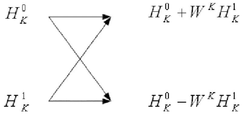
Using (B.5) we will write the …rst equation in (B.4) as Hk= Hk0+ W k_H1 k k = 0,1,..., N 2 1 Hk+(1=2)N = Hk0 W k_H1 k k = 0,1,..., N 2 1: (B.6)

Figure 3: Butter‡y in FFT algorithm

The calculation in (B.6) can be diagrammed as Figure 3.

Figure3. is called a butter‡y. There are (1=2)N butter‡ies for this stage of the FFT. We observed that the directly computation of Hk0requires (N=2)2

complex multiplications. The same applies to the computation of H1 k.

Fur-ther, there are N/2 additional complex multiplications requires to compute Wk_H1

k. Hence the computataion of Hkrequires 2(N=2)2+N=2 = N2=2+N=2

complex multiplications. This …rst step results in a reduction of the number of multiplications from N2 _{to N}2_{=2 + N=2, which is about a factor of 2 for}

N large.

By computing N=4-point DFTs, we would obtain the N/2-point DFTs H0

k and Hk1 from the relations

H_k0 = H_k00+ (W2)kH_k01, H_k+0 1 4N = H_k00 (W2)kH_k01 H_k1 = H_k10+ (W2)kH_k11, H_k+1 1 4N = H_k10 (W2)kH_k11 (B.7) for k = 0,1,...,(1=4)N 1_{.In (2.7), fH}00 Kg is the (1/4)N-point DFTs of fh0,h4,h8,...,hN 4g, fHk01g is the (1/4)N-point DFTs of fh2,h6,h10,...,hN 2g, fH10

k g is the (1/4)N-point DFTs of fh1,h5,...,hN 3g, fHk11g is the (1/4)

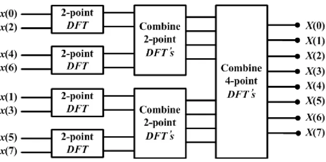
re-Figure 4: FFT algorithm with 8 points

point sequences. For N = 2R_{, this can be performed R = log}

2N times. Thus

the total number of complex multiplications is reduced to (N=2)log2N. The

number of complex additions is N log2N. So, use the FFT algorithm, we

reduce the computation of complex multiplications from N2 to (N=2)log2N:

When N is large, it is a considerable method. Figure 4. is a example of FFT method with N=8.

C.Derivation of the accuracy of the variance analysis

Proof. Note that by Cauchy-Schwarz inequality, E [ Z T 0 e 2rs(@P @x @PF F T @x ) 2_{(s; ~S} s) ~Ss 2 ₂ ds] E [ Z T 0 (e 2rsS~s 2 ₂ )2ds] 1=2 E [ Z T 0 (@P @x @PF F T @x ) 4_{(s; ~S} s)ds] 1=2 ,

where @PF F T

@x is obtained by our FFT option pricing method.

(1) E [ Z T 0 (e 2rsS~s 2 ₂ )2ds] 1=2 = 4 Z T 0 E [(e rsS~s)4]ds 1=2

(by Fubini’s theorem) (e rsS~s = e rsS0e(r+ 1 2 2)s+ W~s = S 0e 1 2 2s+ W~s) = 4 Z T 0 E [(S0e 1 2 2_{s+ W}~_s )4]ds 1=2 = S₀4 4 Z T 0 E [e2 2s+4 W~s_]ds 1=2 = S₀4 4 Z T 0 e10 2sds 1=2 = 1 10S 4 0 2(e10 2_s 1) 1=2 (2) E [ Z T 0 (@P @x @PF F T @x ) 4_{(s; ~S} s)ds] E [ Z T 0 ( @P @x @PF F T @x ) 4_{(s; ~S} s)ds], note @P @x @PF F T @x ~ Ss exp( k) exp((r + 1₂ 2_{)(T s) )} N (1 exp( 2 _{(T t) ))} exp( 1 2 2_{(T s)(N )}2_{) exp(} 2 _{(T s) N )} + 1 X j=1

[exp( j) + exp( j) exp( pk) ~ Ssexp((r + 1 2 2_{)(T s)p +} 2_{(T s)} 2 p 2_)]: And ~ Ss exp( k) exp((r + 1₂ 2_{)(T s) )} N (1 exp( 2 _{(T s) ))} exp( 1 2 2 (T s)(N )2) exp( 2 (T s) N ) 1 U ~ Ss exp((r + 1 2 2_{)(T s) )}

where U = N is the truncated upper bound and for some constant D1.

The other series term

1

X

j=1

[exp( j) + exp( j) exp( pk) S~sexp((r +

1 2 2_{)(T s)p +} 2(T s) 2 p 2_)] = 1 X j=1

exp( j) + exp( pk) ~Ssexp((r +

1 2 2_{)(T s)p +} 2(T s) 2 p 2₎ 1 X j=1 exp( j). Note that 1 X j=1 exp( j) = exp( ) 1 exp( ) 1 1 exp( )

exp( ) (if is small enough) .

Then

1

X

j=1

[exp( j) + exp( j) exp( pk) S~sexp((r +

1 2 2_{)(T s)p +} 2(T s) 2 p 2_)] (1 + ~Ssexp((r + 1 2 2_{)(T s)p +} 2(T s) 2 p 2₎₎

(1 + ~Ssexp(D2(T s))) for some constant D2.

Finally, E [ Z T 0 ( @P @x @PF F T @x ) 4_{(s; ~S} s)ds] = Z T 0 [E ( @P @x @PF F T @x ) 4 (s; ~Ss)]ds Z T 0 [E (1 U ~ Ss exp(D1(T s)) + (1 + ~Ssexp(D2(T s))))4]ds Z T 0 [E 8(1 U ~ Ss exp(D1(T s))4+ 8( (1 + ~Ssexp(D2(T s)))))4]ds Z T 0 E [8(1 U ~ Ss exp(D1(T s))4]ds + Z T 0 E [8( ~Ssexp(D2(T s)))))4]ds = 8 4 U4 Z T 0 exp(4D1(T s))E [ ~Ss 4 ]ds + 484 Z T 0 exp(4D2(T s))E [ ~Ss 4 ]ds,

since E [ ~Ss 4

] and E [ ~Ss 4

] are bounded, there exists F1 and F2 such as

E [ ~Ss 4 ] F1 and E [ ~Ss 4 ] F2, then 84 U4 Z T 0 exp(4D1(T s))E [ ~Ss 4 ]ds + 484 Z T 0 exp(4D2(T s))E [ ~Ss 4 ]ds 84 U4 Z T 0 F1exp(4D1(T s))ds + 484 Z T 0 F2exp(4D2(T s))ds = F1 84 U4 1 4D1 (1 exp(4D1T ) F2 484 1 4D2 (1 exp(4D2T )

8

Reference

[1].Alan V. Oppenhein, Ronald W. Schafer, and John R. Buck,“Discrete-time Signal Processing”, second eddition, Prentice Hall, 1989.

[2].Andrey Itkin, “Pricing Option with VG model using FFT”, working paper, 2007.

[3].David.S.Bates, “Jump and Stochastic Volatility: Exchange Rate Process Implicit in PHLX Deutschemark Options”, working paper, 1993.

[4].Dilip.B.Madan, Peter.P.Carr, and Eric.C.Chang, “The Variance Gamma Process and Option Pricing”, European Finance Review 2: 79–105, 1998.

[5].James S. Walker, “Fast Fourier Transforms”, 1991. [6].Jean Bertoin, “Levy Process”, Cambridge, 1998.

[7].Jean-Pierre Fouque and Chuan-Hsiang Han, “A Martingale Control Variate Method for Option Pricing with Stochastic Volatility”, ESAIM

Prob-[8]. James W. Cooley and John W. Tukey, “An Algorithm for the Machine Calculation of Complex Fourier Series”, Mathematics of Computation, Vol. 19, No. 90, pp 297-301, 1965.

[9].John Hull, “Options, Futures, and other Derivatives”, …ve eddition, Prentice Hall, 2004.

[10].Longsta¤ and Schwarz, “Valuing American Options by Simulation: A Simple Least-Squares Approach,”Review of Financial Studies14: 113-147, 2001.

[11].Marc Avedissian and Eymen Errais, “Option Pricing with Fourier Transform”, working paper , 2002.

[12].B.Oksendal, “Stochastic Di¤erential Equations: An introduction with Applications,” Universitext, 5th edn, Springer, 1998.

[13].Paul Glasserman, “Monte Carlo methods in …nancial engineering ”, Springer, 2004.

[14].Peter Carr and Dilp B. Madan, “Option Valuation Using the Fast Fourier Transform”, 1999.

[15].Roger W. Lee, “Option Pricing by Transform Method: Extensions, Uni…cation, and Error Control”, Journal of Computation Finance, 7(3) pp 51-86, 2004.

[16].L.C.G. Rogers, “Monte Carlo Valuation of American Option,”Math. Finance, 12, 271-286, 2002.

[17].Robert.C.Merton, “Option Pricing When Underlying Stock Returns are Discontinuous”, working paper, 1975.