利用聲光調變器產生穩定Q開關鎖模摻鐿光纖雷射之研究

(1)

國立交通大學

光電工程研究所

碩士

碩士學位

學位

學位論文

論文

利用

利用聲光調變器產生穩定

聲光調變器產生穩定

聲光調變器產生穩定 Q

聲光調變器產生穩定

QQ

Q 開關鎖模

開關鎖模

摻鐿光纖雷射之研究

Stable Q-switched mode-locked Yb-fiber

laser by AO modulation

研

究

生

生：

生

：

：顏子翔

顏子翔

指導教授

指導教授：

：

：賴暎杰

：

賴暎杰

中華民國九十

中華民國九十八

八

八年六月

八

年六月

(2)

利用

利用聲光調變器產生穩定

聲光調變器產生穩定

聲光調變器產生穩定 Q

聲光調變器產生穩定

QQ

Q 開關鎖模摻鐿光纖雷射之研究

開關鎖模摻鐿光纖雷射之研究

Stable Q-switched mode-locked Yb-fiber laser by AO modulation

研究生：顏子翔 Student：Tzu-Hsiang Yen

指導教授：賴暎杰老師 Advisor：Yin-Chieh Lai

國立交通大學

光電工程研究所

碩士論文

A Thesis

Submitted to Institute of Electronics College of Engineering National Chiao Tung University

in partial Fulfillment of the Requirements for the Degree of

Master

In Electro-Optical Engineering

June 2009

Hsinchu, Taiwan, Republic of China

(3)

摘

要

論文名稱：利用聲光調變器產生穩定 Q 開關鎖模摻鐿光纖雷射之研究

校所別：國立交通大學光電工程研究所頁數：1 頁

畢業時間：九十七學年度第二學期學位：碩士

研究生：顏子翔指導教授：賴暎杰老師

在本論文中，我們藉由聲光調變器和線性光纖共振腔在摻鐿的光纖雷射系

統中達到穩定的 Q 開關鎖模雷射運作。在 Q 開關的封包內，我們觀察到鎖模脈

衝的重複頻率為 40 MHz，與聲光調變器內部聲波的頻率相同。在實驗上，我們

也發現 Q 波包的寬度與對稱性取決於聲光調變器外加的調變頻率。當外加頻率

變低的時候，我們觀察到 Q 開關的波包有衛星脈衝的產生，而且它的數目也與

外加的調變頻率有關係。藉由改變在聲光晶體上的光束大小，我們證明了鎖模

脈衝的啟動機制是由聲光調變器振幅調變的作用所產生之諧波鎖模。

(4)

ABSTRACT

Title：Stable Q-switched mode-locked Yb-fiber laser by AO modulation

Pages：1 Page

School：National Chiao Tung University

Department：Institute of Electro-Optical Engineering

Time：July, 2009 Degree：Master

Researcher：Tzu-Hsiang Yen Advisor：Prof. Yin-Chieh Lai

In this thesis, reliable Q-switched mode-locking in an Yb-doped fiber laser is demonstrated by employing an acousto-optic modulator (AOM) and a linear fiber cavity. Within the Q-switched envelope, mode-locked pulses with the repetition rate of 40 MHz can be obviously seen and their repetition rate is equal to the RF driving frequency of the AOM. In our experimental observation, the width and the asymmetry ratio of the Q-switched envelopes depend on the modulation frequency of AOM. At lower modulation frequencies, satellite pulses can be seen with their number being also related to the modulation frequency of AOM. By alternation the optical focus spot size on the AO crystal, we demonstrate that the amplitude modulation of the AOM plays the dominant role for starting the harmonic mode-locking of the laser.

(5)

ACKNOWLEDGEMENT

在這兩年的碩士生涯中，我學習到了很多寶貴的知識以及做人處事的道理。首先我最想感謝的就是我的指導教授賴暎杰老師，在我兩年的研究過程中耐心地給予了我很多的指導及鼓勵，並教導了我解決困難的思考方法及態度，是我在求學期間最大的收穫。特別要感謝林家弘學長和徐桂珠學姊，在實驗期間不斷的指導我並教導我正確的研究態度。感謝項維巍學長、許宜蘘學姐、郭立強學長、鞠曉山學長、張宏傑學長、莊佩蓁學姐、辛宸瑋學姐和陳厚仁學長在課業和實驗上的指導與幫助。另外感謝實驗室的夥伴們昱勳、佩芳、秀鳳、柏萱、家豪、柏崴、姿媛，與他們在課業和研究上的互相幫忙，以及生活上的互相扶持與鼓勵，讓我的研究生活過得如此多彩多姿。感謝鎮岳、哲政和光電系 97 級的同學們，謝謝你們一路上的陪伴與支持。最後我要感謝我的家人們對我全力的栽培及鼓勵，以及所有幫助過我的人，以此獻上我無限的敬意與感激。

(6)

Abstract (in Chinese)

i

Abstract (in English)

ii

Acknowledgement

iii

List of Figures

vi

Chapter 1 :

Introduction

1.1 Progress of Yb-doped fibers 1 1.2 Pulse generation in Yb-doped fiber lasers 2 1.2-1 Q-switched pulse generation 3 1.2-2 Mode-locked pulse generation 4

1.3 Motivation 5

1.4 Organization of the thesis 7

References 8

Chapter 2 :

Principles 2.1 Principle of AO modulation 11 2.1-1 Acousto-optic effects 11 2.1-2 Bragg Condition 12 2.1-3 Modulation 15 2.2 Theory of Q-switching 17 2.3 Mode-locking by amplitude modulation 22

2.3-1 Mode-locking 22

2.3-2 Amplitude modulation 25

References 30

Chapter 3 :

Experimental results

3.1 Q-switched pulse generation 31 3.1-1 Experimental setup 31 3.1-2 Results and discussions 32 3.2 Q-switched mode-locked pulse generation 36 3.2-1 Experimental setup 36 3.2-2 Results and discussions 37

3.3 Analysis 48

(7)

Chapter 4 :

Conclusions 52

(8)

LIST OF FIGURES

Fig. 2.1 The refractive index variation in an AO medium caused harmonic sound wave and the interaction which the acoustic wave can diffract the optical wave [2.3]...11 Fig. 2.2 Reflections from stratified refractive index of an inhomogeneous

medium [2.3]………...13 Fig. 2.3 The Bragg condition by vector relation for upshifed and downshifed

case………...14 Fig. 2.4 The optical wave incident normally into a thin acoustic wave is

deflected into two directions [2.3]……….…….…………15 Fig. 2.5 (a) An acousto-optic modulator (b) An acousto-optic switch [2.3]………16 Fig. 2.6 Interaction of an optical beam of angular divergence with an acoustic

plane wave of frequency in the band f0 ± B. Many parallel q vectors

of different lengths may match a direction ofthe incident light

[2.3]………..……...17 Fig. 2.7 The loss modulation, population inversion and the pulse generation of

Q-switch lasers [2.3]………...………….……18 Fig. 2.8 The geometrical setup and the detailed process of pulse formation in

the time domain for a Q-switched laser [2.1]………..19 Fig. 2.9 The time and frequency domain representations of a mode-locked

laser [2.1]……….…24 Fig. 2.10 The amplitude modulation or loss modulation of active

mode-locking process………....…26 Fig. 3.1 Schematic diagram of the Q-switched ytterbium fiber laser……….……..31 Fig. 3.2 Time traces of Q-switched pulse trains at 120 kHz modulation

(9)

frequency and the 300 mW pump power………...…...32 Fig. 3.3 Time traces of Q-switched pulse trains at (a) 40 kHz (b) 70 kHz (c)

100 kHz………...……33 Fig. 3.4 The formation of satellite pulses at long switch off time

Duration………..….34 Fig. 3.5 Schematic diagram of the Q-switched mode-locked ytterbium fiber

laser………..….…..36 Fig. 3.6 (a) Time traces of Q-switched pulse trains at 100 kHz (b) Expanded

time trace of single Q-switched envelope. The corresponding

optical spectrum is shown in the inset………...…38 Fig. 3.7 Time traces of Q-switched pulse trains at (a) 5 kHz (b) 10 kHz (c) 20

kHz (d) 30 kHz (e) 40 kHz (f) 60 kHz………...…...39 Fig. 3.8 Expanded temporal shape of a single Q-switched & mode-locked

pulse trains with 188 mW pumping at (a) 10 kHz (b) 60 kHz and (c) 100 kHz………...………...……41 Fig. 3.9 Measured widths and estimated peak power of Q-switched envelopes

versus different AOM frequencies at the pump power of 188

mW………...……….…43 Fig. 3.10 The comparison of pulse widths and peak power of Q-switched

envelopes at (a) low and (b) high AOM frequencies……….………...43 Fig. 3.11 Time traces of Q-switched pulse trains at 100 kHz for (a) 100 mW

(b) 130 mW (c) 180 mW pump power………...45 Fig. 3.12 (a) Time traces of Q-switched and mode-locked pulse trains at 100

kHz (b) Expanded time trace of single Q-switched envelope…………..46 Fig. 3.13 (a) Time traces of Q-switched and mode-locked pulse trains at 100

(10)

envelope.……….………...…47 Fig. 3.14 The comparison of the Q-switched pulse trains at 100 kHz and 188

mW pump power between using (a) 12 cm focal lens and (b) 7.5 cm focal lens……….……….………..48 Table 3.1 The rising time t1, the falling time t2, the pulse widths τ and the

peak power of Q-switch envelopes………..…….42 Table 3.2 Pulse width of Q-switch envelopes calculated from Q-switch laser

(11)

Chapter 1 Introduction

1.1 Progress of Yb-doped fibers

It has been of considerable interest in studying Yb-doped fiber lasers because of their beneficial properties for applications around the 1 µm wavelength. In particular, Yb-doped materials have attracted much attention as possible laser gain media since they typically have a number of advantageous properties such as high quantum efficiency, absence of ground-state absorption and excited-state absorption, and a long upper-state lifetime. One practical feature of Yb ions is that they can be pumped in the convenient pumping bands around 915 and 980 nm. As a result of these properties, the Yb-doped fibers seem likely to supersede the Nd-doped fibers which also emit near 1 µm. In addition, the efficiency and broad gain spectrum of Yb-doped fibers also make them attractive for short-pulse operation. In this respect, the generation of 100-fs pulses from Yb fiber lasers has been reported [1.1].

Due to the wide gain bandwidth, ultrashort pulse generation in Yb-doped fiber lasers has been investigated by employing different mode-locking techniques.[1.2,1.3,1.4] Moreover, Q-switched operation of Yb-doped fiber lasers is also of interest because the relatively long upper-state life-time of Yb can help the storage of energy from efficient diode pumping sources [1.5].

The first report of laser action by using Yb-doped silicate glasses was in 1962 [1.6]. However, in the beginning Yb3+ as a laser-active ion has attracted relatively little interest. Despite the use of stretched-pulse techniques and double-clad gain fibers, the pulse energies obtained from Yb fiber lasers were an order of magnitude lower than those obtained with single-mode erbium and neodymium fiber lasers in earlier studies [1.7]. Theoretically, Yb

(12)

fiber lasers should be capable of providing larger energies than Er fiber lasers. Thus the potential of short-pulse Yb fiber lasers was not fulfilled until recently.

In the recent years, several advances in the performance of Yb fiber lasers have been reported. Lim et al succeeded to produce the first mode-locked Yb fiber laser to generate pulse energies of ~1 nJ. The performances of Yb fiber lasers were now comparable to those obtained with Er and Nd fibers. Pulses as short as 52 fs have also been reported [1.1]. Then Ilday et al. were able to demonstrate an Yb fiber laser that generates 50-fs pulses with 5 nJ pulse energy by suppressing the wave-breaking effects of solitonlike pulse shaping at high pulse energies [1.2]. The 80-kW peak power of this laser is five times the previous maximum peak power from a femtosecond fiber laser. These lasers are stable and reliable instruments that employ only single-mode fibers and are pumped in-core by diodes. Lim et

al. [1.1] and Ilday et al. [1.2] have used the diffraction gratings for the control of

group-velocity dispersion (GVD) in the laser cavity. As a step toward an integrated source, Lim et al. [1.8] demonstrated an Yb fiber laser that employed photonic-crystal fibers for dispersion control. This laser generated 1 nJ and 100 fs pulses but was not self-starting [1.8]. By optimizing the group-velocity dispersion of the laser, pulses as short as 36 fs are generated. This is shorter than the shortest pulses produced by the Er fiber laser (-63 fs) and the Nd fiber laser (-42 fs) [1.9]. To date, these results are the shortest pulses generated by a fiber laser.

1.2 Pulse generation in Yb-doped fiber lasers

The methods of generating pulses in lasers can be divided into two types for a variety of applications and purposes: Q-switching and CW mode-locking. There is a main difficulty associated with pulse generation in Yb-doped fibers: the high value of normal material dispersion of silica at wavelengths below 1.1µm [1.10]. Although waveguide dispersion has

(13)

generally been used to balance material dispersion at longer wavelengths (1.3µm), it does not appear feasible to achieve overall anomalous dispersion by this approach for such a short wavelength. Some techniques can be used to achieve the Q-switched pulse generation and mode-locked pulse generation easily. Simultaneous Q-switched mode-locked operation of the lasers possess the superior property of high peak power over CW mode-locked lasers, which has been widely reported for diode pumped all solid state lasers (DPSSL) [1.24] but not so widely for fiber lasers. This will be the main subject to be explored in the present thesis work.

1.2-1 Q-switched pulse generation

High-power Q-switched fiber lasers with nanosecond pulse durations are of great interest in applications such as laser micromachining, material processing, nonlinear optics, and laser sensing. The mechanism of Q-switched pulse generation is achieved by placing a modulator to produce periodical on-off modulating of the resonator loss. Generally, active and passive devices, such as acousto-optic modulators, electro-optic modulators and saturable absorbers (Cr4+:YAG), have been reported to be used in Yb-doped fiber lasers for generating Q-switched pulses.

Q-switching in Yb-doped fiber laser can be realized in an active way by acousto-optic modulation [1.11-1.16] or electro-optic modulation [1.17]. The advantage of the active Q switched method is the easy control of the pulse repetition rate and the pulse width, whereas the disadvantage is the requirement of an additional optical modulator. Through acousto-optic modulation, the sound wave will modulate the optical wave proportionally. By varying the sound wave on and off, the loss inside the cavity will also vary accordingly so as to generate the giant Q-switched pulses. The principle of electro-optic modulation is based on the linear electro-optic effect that can modify the refractive index of a nonlinear

(14)

crystal by an electric field in proportion to the field strength. In electro-optic modulators, an electro-optic crystal is used as a voltage-controlled gate inside the optical configurations that can be used to control the power, phase or polarization of a laser beam.

Passive Q-switching in Yb-doped fiber lasers by using saturable absorbers such as Cr4+:YAG have also been reported [1.18]. Cr4+:YAG is an ideal saturable absorber material at 1 µm with large absorption cross section, low saturation intensity, high thermal conductivity and damage threshold, and good chemical and photochemical stability. The absorber’s opacity decreases as the increasing optical intensity, which prevents rapid inversion depletion due to high loss at the early stage of oscillation since the pump intensity is not enough to saturate the absorption.

1.2-2 Mode-locked pulse generation

In order to obtain pulses with higher peak power, the mode-locking techniques can be used to lock the phases of all oscillating modes to form giant narrow pulses in the time domain. Passive mode-locking by using semiconductor saturable absorber mirrors (SESAM), polarization additive pulse mode-locking (P-APM) configurations and nonlinear optical loop mirrors (NOLM) have been frequently reported in Yb-doped fiber laser systems. The principles of P-APM and NOLM exploit nonlinear effects induced by self-phase and cross-phase modulation, both resulted from the optical Kerr effect.

Passive mode-locking by utilizing a semiconductor saturable absorber mirror is robust and also widely used in many Yb-doped fiber laser studies [1.19]. The optical absorption excites electrons from the valence band to the conduction band. As electrons accumulate in the conduction band, the absorbing transition is depleted and therefore the net absorption is reduced.

(15)

lasers. There have been a lot of researches in P-APM mode-locked Yb-doped fiber lasers during recent years [1.7]. The two light polarization components are added together at the polarizer where the peak of the pulse with more nonlinear rotation transmits at low loss and the wings are blocked. The action is very fast and its strength is adjustable by the polarization controllers. However it may suffer from the drift of polarization settings with respect to temperature change such that readjustment is almost necessary.

Mode-locking by a nonlinear optical loop mirror has been one of the most influential methods to date, resulting in pulses as short as 125 fs [1.20-1.21]. The power imbalance between the counter propagating beams results in a difference in the nonlinear phase shifts of the two beams caused by the self-phase modulation. The mode-locking operation of the laser is due to the intensity dependent reflectivity of the NOLM.

1.3 Motivation

Q-switched and mode-locked (QML) operation of Yb-doped fiber lasers possess a variety of applications such as range finding, optical time domain reflectometry, remote sensing, medical and industrial processing. This is because they have higher peak powers than CW mode-locked lasers. Acousto-optic modulators have been widely used for active Q-switching with the linear Fabry-Perot or the ring cavity configuration in the laser systems [1.15].

In solid state lasers, the fully modulated QML operation has been demonstrated in the diode pumped Nd:YVO4 laser modulated by an acousto-optic modulator [1.21]. The

acousto-optic modulator was located near flat output mirror that played a dual role of Q-switcher and Mode-locker to generate pulse trains with 3 W average output power and 130 µJ pulse energy. Each envelope has approximately 5-8 mode-locked pulses inside. In

(16)

Er-doped fiber laser, a Q-switched erbium doped single-mode fiber laser is demonstrated by using AOM and is optimized for high power operation [1.22]. At the 1 kHz repetition rate, the laser generates 8 ns pulses with 230 W peak power. The self-mode-locked pulses are produced through mode beats between axial modes [1.23]. The self-phase modulation induced as the pulses propagate through the single mode fibers result in the spectral broadening in the Q-switched erbium-doped fiber laser. At the 1.6 kHz repetition rate and 350 mW absorbed power, the highest peak power of the emitted pulses is 200 W.

A large number of studies have been made on Yb-doped fiber lasers with AOM to generate Q-switched pulses. In the contrast, little has been reported on simultaneous Q-switched and mode-locked operation of the Yb-doped fiber lasers. The output pulse characteristics of Q-switched Yb-doped fiber lasers have been experimentally investigated by Y. Wang [1.11-1.14] and others [1.16]. At a fixed modulation frequency, with a fine adjustment of acousto-optic modulation window ON time, pump power and cavity mirror position, the modulation free single-peak pulse, multi-peak pulse, mode-locked resembling pulse and multi-pulse structured pulse shapes can be obtained in a Q-switched fiber laser [1.15]. The multi-peak or split pulse is due to the nonlinear phenomena such as stimulated Brillouin scattering (SBS) and Simulated Raman Scattering (SRS). By carefully adjusting the position of the mirror near the AOM, they also show a periodically modulated mode-locked resembling pulse shape at the 32 kHz modulation frequency. The mode beating between the round-trip frequency-shifted beam at ω+2Ω from the AO Q-switch and the original (un-deviated) beam at ω, has been shown to cause the mode-locked resembling output pulses.

To generate stable Q-switched mode-locked pulses with full modulation depth in Yb-doped fiber laser systems by AOM will have important practical applications. Therefore, in this thesis, we try to optimize the arrangement of the whole cavity setup for investigating simultaneous QML generation in an Yb-doped fiber laser modulated by an AOM. The characteristics of QML pulses are studied and the mode-locking mechanism is also

(17)

investigated experimentally.

1.4 Organization of the thesis

The present thesis is consisted of four chapters. Chapter 1 is an introduction of the past progress on pulse generation in Yb-doped fiber lasers and the motivation for doing this research. Chapter 2 describes the principles and theories of acousto-optic modulation, Q-switching, mode-locking and amplitude modulation. Chapter 3 demonstrates our experimental setup and results. The discussion and analyses of our results are also presented. Finally, Chapter 4 gives the conclusions.

(18)

References

[1.1] H. Lim, F. O. Ilday, and F. W. Wise, “Generation of 2-nJ pulses from a femtosecond Yb fiber laser,” Opt.Lett. 28, 660-662 (2003).

[1.2] F. O. Ilday, H. Lim, J. R. Buckley, F. W. Wise, and W. G. Clark, “Generation of 50-fs, 5-nJ pulses at 1.03 µm from a wave-breaking-free fiber laser,” Opt. Lett. 28, 1365-1367 (2003)

[1.3] R. Hohmuth,W. Richter, A. T¨unnermann, “Self-starting self-similar all-polarization maintaining Yb-doped fiber laser,” Opt. Express, 13, 9346-9351 (2005).

[1.4] X. Zhou, D. Yoshitomi, Y. Kobayashi, and K. Torizuka, “Generation of 28-fs pulses from a mode-locked ytterbium fiber oscillator,” Opt. Express 16, 7055-7059 (2008).

[1.5] J. A. Alvarez-Chavez, H. L. Offerhaus, J. Nilsson, P. W. Turner, W. A. Clarkson, and D. J. Richardson, “High-energy, high-power ytterbium-doped Q-switched fiber laser,” Opt. Lett. Vol. 25, No. 1 (2000)

[1.6] H. W. Etzel, H. W. Candy. and R. J. Ginther, “Stimulated emission of infrared radiation from ytterbium-activated silicate glass,” Appl. Opt., vol. 1, pp. 534, 1962

[1.7] V. Cautaerts, D. J. Richardson, R. Paschotta, and D. C. Hanna, “Stretched pulse Yb3+:silica fiber laser,” Opt. Lett. 22, 316 (1997)

[1.8] H. Lim, F. O. Ilday, and F. W. Wise, ”Femtosecond ytterbium fiber laser with photonic crystal fiber for dispersion control,” Opt. Exp. 10, 1497-1502 (2002).

[1.9] F. Ö. Ilday, J. Buckley, L. Kuznetsova, and F. W. Wise, “Generation of 36-femtosecond pulses from a ytterbium fiber laser,” Opt. Express. 3550, Vol. 11, No. 26 (2003)

[1.10] O. G. Okhotnikov, L. Gomes, N. Xiang, and T. Jouhti, “Mode-locked ytterbium fiber laser tunable in the 980–1070 nm spectral range,” Opt. Lett., Vol. 28, No. 17 (2003) [1.11] Y. Wang and Chang-Qing Xu, “Modeling and optimization of Q-switched double-clad

(19)

[1.12] Y. Wang and Chang-Qing Xu, “Understanding multipeak phenomena in actively Q-switched fiber lasers,” Opt. Lett. 29, 1060-1062 (2004).

[1.13] Y. Wang and Chang-Quing Xu, “Switching-induced perturbation and influence on actively Q-switched fiber lasers,” IEEE J. Quantum Electron. 40, 1583-1596 (2004). [1.14] Y. Wang, Alejando Martinez-Rios and Hong Po, “Pulse evolution of a Q-switched

ytterbium-doped double-clad fiber laser,” Opt. Eng. 42, 2521-2526 (2003).

[1.15] B. N. Upadhyaya, U. Chakravarty, A. Kuruvilla, K. Thyagarajan, M. R. Shenoy, and S. M. Oak1, “Mechanisms of generation of multi-peak and mode-locked resembling pulses in Q-switched Yb-doped fiber lasers,” Opt. Express. 11576.

[1.16] H. Zhao, Q. Lou, J. Zhou, F. Zhang, J. Dong, Y. Wei, G. Wu, Z. Yuan, Z. Fang, and Z. Wang, ”High-Repetition-Rate MHz Acoustooptic Q-Switched Fiber Laser,” IEEE Photon. Techno. Lett., Vol. 20, No. 12 (2008)

[1.17] Amnon Yariv, Pochi Yen, “Photonics,” sixth edition, New York Oxford university press 2007.

[1.18] L. Pan, I. Utkin, and R. Fedosejevs, Senior Member, IEEE, ”Passively Q-switched Ytterbium-Doped Double-Clad Fiber Laser With a Cr4+:YAG Saturable Absorber,” IEEE Photon. Techno. Lett., Vol. 19, No. 24 (2007)

[1.19] L. A. Gomes, L. Orsila, T. Jouhti, and O. G. Okhotnikov, “Picosecond SESAM-Based Ytterbium Mode-Locked Fiber Lasers,” IEEE J. Select. Topics Quantum Electron, Vol. 10, No. 1 (2004)

[1.20] M. Salhi, A. Haboucha, H. Leblond, and F. Sanchez, “Theoretical study of figure-eight all-fiber laser,” Phys. Rev. A 77, 033828 (2008)

[1.21] B. Ibarra-Escamilla, O. Pottiez, E. A. Kuzin, R. Grajales-Coutiño, and J. W. Haus, “Experimental Investigation of a Passively Mode-Locked Fiber Laser Based on a Symmetrical NOLM with a Highly Twisted Low-Birefringence Fiber,” Laser Phy., Vol. 18, No. 7 (2008)

(20)

[1.21] J. K. Jabczyński, W. Zendzian, J. Kwiatkowski, “Q-switched mode-locking with acousto-optic modulator in a diode pumped Nd:YVO4 laser,” Opt. Express 2184, Vol.

14, No. 6 (2006)

[1.22] P. Myslinski, J. Chrostowski, J. A. Koningstein, and J. R. Simpson, "High power Q-switched erbium doped fiber laser," IEEE J. Quantum Electron. 28, 371-377 (1992) [1.23] P. Myslinski, J. Chrostowski, J. A. Koningstein, and J. R. Simpson, “Self-mode locking

in a Q-switched erbium-doped fiber laser,” Appl Opt, Vol. 32, No. 3(1993)

[1.24] J-H. Lin, H.-R. Chen, H.-H. Hsu, M.-D. Wei, K.-H. Lin, and W.-F. Hsieh, “Stable Q-switched mode-locked Nd3+:LuVO4 laser by Cr4+:YAG crystal,” Opt. Express. 16,

16538-16545 (2008)

[1.25] J.-H. Lin, K.-H. Lin, H.-H. Hsu, and W.-F. Hsieh, “Q-switched and mode-locked pulses generation in Nd:GdVO4 laser with dual loss-modulation mechanism,” Laser Phys. Lett.

5, 276-280 (2008).

(21)

Chapter 2 Principles

2.1 Principle of AO modulation

2.1-1 Acousto-optic effects

An acousto-optic crystal is an optical medium which refractive index can be altered by the presence of sound. In other words, sound will modifies the effects of the medium on light. The mechanism by which sound can control light is called the acousto-optic effect and is used by a lot of devices.

Fig. 2.1 The refractive index variation in an AO medium caused by a harmonic sound wave and the interaction which the acoustic wave can diffract the optical wave [2.3].

As pictured in Fig. 2.1, the sound wave is a harmonic plane wave of density vibration in a medium so that the refractive index can be changed periodically. It is a dynamic strain involving molecular vibration that takes the form of waves which travel at a velocity of sound

(22)

characteristics in the medium. The refractive index is larger when the density is higher in those regions where the medium is compressed. On the contrary, in the decompressed region, its density and refractive index are smaller. In solids, sound involves vibrations of the molecules about their equilibrium positions, which will alter the optical polarizability and consequently the refractive index. So an acoustic wave make the medium become inhomogeneous with a time-varying stratified refractive index.

With taking the two significantly different time scales for light and sound into account, the variations of the refractive index in an acousto-optic medium caused by sound are usually very slow in comparison with an optical period since optical frequencies are much greater than acoustic frequencies. As a consequence, we can always treat the material as if it were a static inhomogeneous medium.

2.1-2 Bragg Condition

Based on the above assumption, the medium is like the stratified parallel planes representing refractive-index variations created by an acoustic plane wave which can be regard as a Bragg grating with the wavelength equal to the sound wavelength Λ. Thus the interaction of light and sound is the Bragg reflection (Bragg diffraction) of the optical plane wave. The Bragg grating created by an acoustic wave will reflect light if the optical wave angle of incidence θ satisfies the Bragg condition for constructive interference as illustrated in Fig. 2.2,

sin

2

B

θ

λ

θ

=

Λ

(2.1) where λ is the wavelength of light in the medium and θB = sin-1(q/2k) is at the Bragg angle

θB.

(23)

traveling in the x direction in a medium with velocity vs, radio frequency (RF) f, and

wavelength Λ= vs/f. The relative displacement at position x and time t is

0

( , )

cos(

)

s x t

=

S

Ω −

t

qx

(2.2)

where S0 is the amplitude, Ω = 2πf is the angular frequency and q=2π/Λ is the wavenumber.

Thus the medium has a time-varying inhomogeneous refractive index in the form of a wave

0

( , )

cos(

)

n x t

= − ∆

n

Ω −

t

qx

(2.3) with amplitude ₀

1

3 ₀

2 n

ρ

n S

∆

=

(2.4) where ρ is a phenomenological coefficient known as the photoelastic constant.

In addition to the type of traveling wave in acoustic wave, standing wave is another type used in acoustic wave. The acoustic strain of standing wave s(x,t) is periodic, with a spatial period equal to the acoustic wavelength:

0

( , )

cos(

)cos( )

s x t

=

S

Ω

t

qx

(2.5)

Fig. 2.2 Reflections from stratified refractive index of an inhomogeneous medium [2.3].

(24)

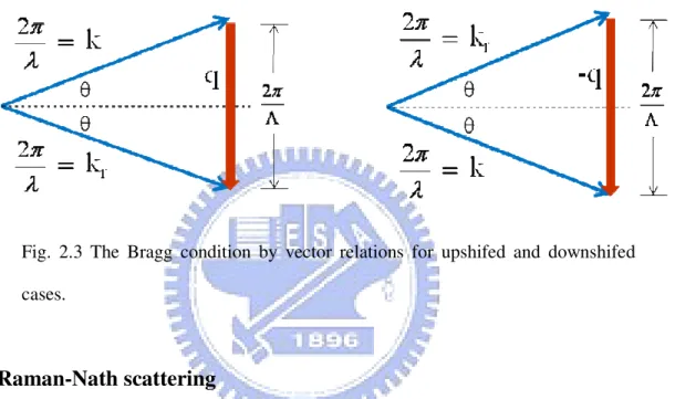
of the sound wave and the incident, reflective optical waves. The condition q = 2ksinθB is

equivalent to the vector relation as shown below r

k

= +

k

q

for upshifed case (2.6)

r

k

= −

k

q

for downshifed case (2.7) which can be illustrated by the vector diagram as pictured in Fig. 2.3

Fig. 2.3 The Bragg condition by vector relations for upshifed and downshifed cases.

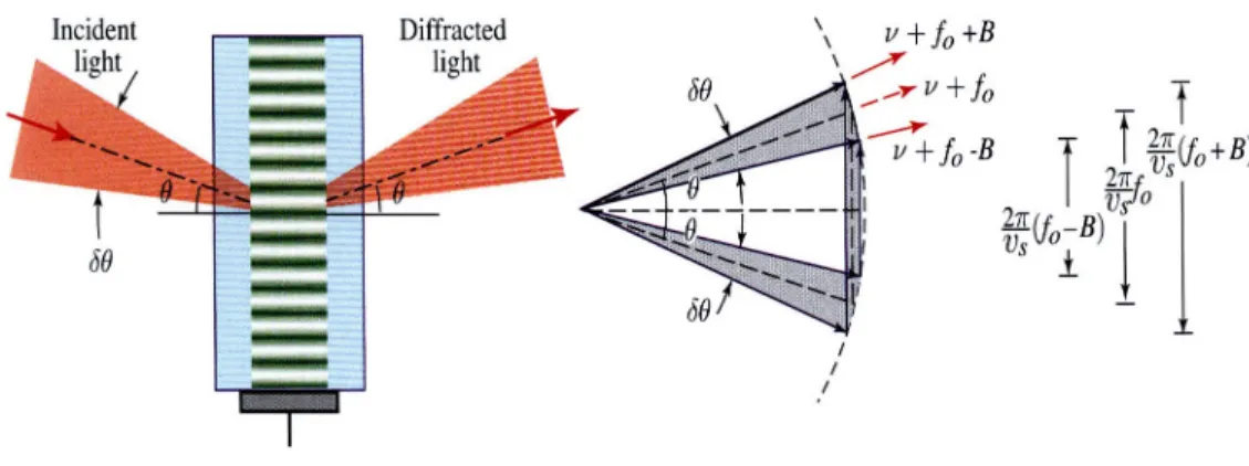
Raman-Nath scattering

We now consider the case which the acoustic beam size is thin. The medium with the thin acoustic beam can diffract light at angles that are significantly different from the Bragg angle. To take a most used example as shown in Fig. 2.4, assume the incident optical plane wave is perpendicular to the direction of a thin acoustic beam, and thus it will be diffracted into zero-th order and first order directions. The diffracted situation by the thin acoustic beam can be regarded as the interference from multi slits. So the constructive interference condition is satisfied if the reflected wavevector kr makes reflected angles ±θ, where θ

satisfied the formula

2 sin

2 θ

λ

=

Λ

(2.8)

(25)

Fig. 2.4 The optical wave incident normally into a thin acoustic wave is deflected into two directions [2.3].

In fact, the incident optical wave is diffracted into plenty of higher diffraction orders by the thin diffraction grating where the angles of the higher-order diffracted waves are ±2θ, ±3θ… etc. The higher-order acousto-optic interaction is through the higher order components of the phase grating induced by the AO effect. Similar interpretations apply to higher orders of diffraction.

The acousto-optic interaction of light with a perpendicular thin sound beam is known as Raman-Nath or Debye-Sears scattering of light by sound.

2.1-3 Modulation

The modulation mechanism by an acousto-optic crystal is by using an electrical signal to drive the acoustic transducer and the intensity of the reflected optical wave can be varied proportionally according to the electrical signal sent to the acoustic transducer. The sound intensity has to be sufficiently weak, and thus the intensity of the reflected light by the Bragg

(26)

grating will be proportional to the intensity of sound. The variation from the electrical signal to the reflected light is linear so that we can modulate the intensity of the optical wave by simply controlling the input electrical signal.

Fig. 2.5 (a) An acousto-optic modulator. (b) An acousto-optic switch [2.3].

As shown in Fig 2.5, increasing the intensity of sound, the reflected light can also be increased simultaneously. When the acoustic power increases enough, total reflection can be achieved and saturation will occur. So we can make the modulator as an optical switch. By switching the acoustic wave on and off, one can turn the reflected light on and off, or oppositely turn the transmitted light off and on, as illustrated in Fig. 2.5(b).

The modulator usually has its bandwidth which is the maximum frequency at which it can efficiently modulate. The sound wave, in fact, is often not single frequency. The amplitude of an acoustic wave at frequency f0 is varied as a function of time by amplitude

modulation with a signal of bandwidth B, so it has frequency components within a band f0 ± B

centered about the frequency f. Now we focus on the incident light which is actually a beam of width D and angular divergence δθ = λ/D. The optical plane wave with the matching Bragg angle will interact with each frequency component of sound as shown in Fig. 2.6.

(27)

Fig. 2.6 Interaction of an optical beam of angular divergence with an acoustic plane wave of frequency in the band f0 ± B. Many parallel q vectors of different

lengths may match a direction of incident light [2.3].

The frequency band f0 ± B can be matched by an optical beam of angular divergence.

(2 / )

2 /

s s

v B

v

π

π λ

λ

δθ

≈

=

(2.9)

And therefore the bandwidth of the modulator is s s

v

B

v

D

δθ

λ

=

(2.10)

The light beam should be focused to a small diameter with the increasing bandwidth of the modulator.

2.2 Theory of Q-switching

The mechanism of Q-switching is by turning on and off the resonator loss periodically. That is to say, by spoiling the resonator quality factor Q, the loss inside the cavity will

(28)

oscillate periodically in order to obtain giant output pulses. So Q-switching can also be called loss switching. One usually introduces the loss oscillation through using a modulated absorber. Because the pump continues to deliver constant power at all time, at the high loss times, energy is stored inside the cavity in the form of an accumulated population inversion. During the on-time, the losses are reduced and the large accumulated population inversion is released, generating giant and short pulses of light as shown in Fig. 2.7.

Fig. 2.7 The loss modulation, population inversion and the pulse generation of Q-switch lasers [2.3].

As shown in figure 2.8, we identify that the shutter is opened at the point of t = 0. The population inversion is far above threshold at that instant in the system. The spontaneous emission along the axis of the cavity is then enormously amplified so that the pulse quickly builds up to a sufficiently strong one through depleting the population inversion.

(29)

d

Shutter

Gain

l

s

l

g

T

a

T

b

T

_c

T

_d

n

s

a

s

n

g

s

R

1

R

2

=1-T

2

A

Fig. 2.8 The geometrical setup and the detailed process of pulse formation in the time domain for a Q-switched laser [2.1].

The giant pulse occurs on a very short time scale with a large number of stimulated photons. In view of this large increase in the photon flux, we realize that the population inversion will become depleted as the photon number increases. Consequently, we must keep track of the number of excited states as well as the number of photons.

We now make numerical predictions about the amplitude of the intensity produced by this Q switching operation. We can get rid of at least two of the transverse spatial coordinates by

(30)

assigning an effective beam area A. We are then left with the two dimensions z and t by ignoring any nonuniformity in the population density or the photon density along the z-axis of the simple cavity.

First of all, we have to inquire the time evolution of the photon number inside the cavity presuming that there are a few around to initiate the lasing process. In one round trip the photon number will increase by a factor exp[2(N2-N1)σlg] and decrease owing to imperfect

window transmission (Πj Tj), finite reflectivity (Πi Ri) and residual absorption (usually in the

shutter) as exp-[2αsls]. The net change in Np during a round trip, the amplified result minus

the starting value, divided by τRT(round trip time) is an excellent approximation to dN_p/dt.

2 1 2( ) 2

[(

)(

)

]

1 {

}

g s sl N N l i j i j P p RT

R

T e

e

dN

N

dt

σ α

τ

+ − −

−

=

⋅

∏

(2.11)

With some abbreviation and approximation,

p p

{

1}

p th

dN

N

n

dt

=

τ

　

n

−

　

(2.12)

where n = (N2-N1)Alg is the total number of inverted atoms in the cavity interacting with an

optical mode of cross sectional area A, and nth is total number at threshold. Equation (2.12)

helps to account for that the photons increase with time if the inversion is larger than the threshold value, and otherwise, they decrease.

The stimulated emission not only increases the photon numbers but also changes the population inversion simultaneously. With a photon producing, there is one atom changing its state from 2 to 1, which reduces the inversion by 2 (for equal degeneracies) and thus reduces the gain. Now that we know how to model the time evolution of the photon number, the next step is to study the dynamics of the population inversion. The equations for the population of the upper and lower state are given by:

(31)

dN

(

)

N

dt

h

σ

ν

= −

−

+ -2 2 1

I +I

（

）

(2.13)

dN

(

)

N

dt

h

σ

ν

= +

−

+ -1 2 1

I +I

（

）　

(2.14)

Subtracting Eq.(2.14) from Eq.(2.13) and with some derivation, the formula of population inversion can be written as

2

p

th p

N

dn

n

dt

= −

n

⋅

τ

(2.15) The above equation could have been stated as a direct consequence of the formula of photon number since it merely states that if the photons increase by 1, then the inversion must decrease by 2.

By substituting a time scale normalized to the photon lifetime of the passive cavity by T = t/τp and dividing Eq.(2.12) by Eq.(2.15), which eliminates time from the equation.

1 (

1)

2

p _th

dN

_n

dn

=

n

−

(2.16)

Now we multiply both sides by dn, integrate the left-hand side from the initial value of the photon number Np(i) (which is negligible compared to what it will be) to the photon number

Np(max) at the peak of the power pulse and simultaneously integrate the right-hand side from

the initial value of the inversion, ni, to the threshold value nth. Thus we can find an

elementary solution for the photon number Np in terms of the population inversion n as shown

below.

(max)

(

)

2

i th th i p th

n

N

ln

n

−

=

−

(2.17) f

exp[ (

i f

)]

t th

n

−

=

−

(2.18)

(32)

output energy, and a reasonable estimation for its FWHM in terms of the photon number Np

and population inversion n without using more complicated mathematical methods. The maximum output power can be expressed in a compact fashion by

(max)

_cpl p

(max)

p

h N

P

η

ν

τ

=

(2.19)

where ηcpl is the coupling efficiency which can be expressed as the ratio of the output mirror

transmission coefficient to the total loss in one round trip. The output energy is

2

i out cpl xtn

n h

W

=

η η

ν

(2.20) where ηxtn is the fraction of the initial inversion converted to photons.

Another important issue to be addressed is to estimate the pulse width. A very reasonable estimate can be obtained by dividing the output energy by the maximum power

(max)

out

W

t

P

∆ ≈

(2.21)

As we will see, the peak intensity can be many times the CW level because this initial population inversion may be many times that required for CW oscillation in the absence of the shutter. We may note that the opening window time and the repetition rate of the shutter will also influence the peak power and pulse width of the giant Q-switch pulses.

2.3 Mode-locking by Amplitude Modulation

2.3-1 Mode-locking

A laser can oscillate on many longitudinal modes, with frequencies that are equally separated by the intermodal spacing ν= c/2d. Mode-locking is a laser mechanism which is

(33)

attained by coupling together these longitudinal modes of a laser and locking their phases to each other. These modes which the phases of these components are locked together behave like the Fourier-series expansion of a periodic function, and therefore constitute a periodic pulse train. We can couple these modes by periodically modulating the losses or gains inside the resonator.

The properties of the mode-locked laser are

1. The laser is emitted in a form of a train of pulses with a period τRT = 2d/c, i.e., the

round-trip transit time, and the repetition rate is 1/τRT.

2. The FWHM of the mode-locked pulse Δtp is usually very short compared toτRT.

Typical pulse widths range from a relatively long nanosecond (10-9 sec) to tens of femtoseconds (10-15 sec).

3._{At the same averaged output power of the CW and mode-locked laser, the peak power of} the mode-locked pulse is roughly τRT /Δtp multiplied by the CW value. In other words,

the peak power is equal to N times the average power, where N is the number of modes locked together. Thus the peak power can be greatly significant even though the average power is similar.

Now we start to discuss the mathematical theory of mode-locking with multilongitudinal mode oscillation. We assume that the central mode is presumed to be at ω0 and there are

(N-1)/2 modes uniformly spaced at ωc = 2π/τRT (mode spacing) on either side of ω0 and thus

there are total N modes in all as shown in Fig. 2.9. The electric field in space can be written as ( 1) / 2 0 ( 1) / 2

( )

N _n

( )exp[ (

_c

)

_n

( )]

N

e t

+ −

E t

j

ω

n

ω

t

φ

t

− −

=

∑

+

(2.22)

where En is the mode amplitude and ψn is the mode phase which is changing slowly

(34)

phase randomly distributed over 2π, the amplitude variation would be very small.

Fig. 2.9 The time and frequency domain representations of a mode-locked laser [2.1].

In order to approach mode-locking, we forced each phase of all modes to a fixed value that might as well be set equal to zero since any constant value amounts to a time shift. Thus the term inωct acts as a phase shift of the nth mode with respect to that at line center. We

assume that all phase term ψn = 0 and all amplitudes are equal to E0, so the electric field can

be shown as 0 0

sin(

/ 2)

( )

[

]

sin(

/ 2)

j t c c

N

t

e t

E e

t

ω

=

(2.23)

(35)

2 2 0 0 0

sin(

/ 2)

( )

* ( )

( )

[

]

2

2 sin(

/ 2)

c c

E

N

t

e t

e

t

I t

t

ω

η

ω

⋅

=

(2.24) We can find that the intensity is N2 times the intensity per mode when ωct/2 is an integral

multiple of π. Therefore the average power of the laser is larger than the power per mode N times. And thus we obtain the (approximate) relation that the peak power is N times the average.

peak ave

P

=

N

×

P

(2.25) The pulse width is estimated by using

P

_peak

⋅ ∆

t

_p

≈

P

_ave

⋅

τ

_RT (2.26) With substituting the average power and the number N of oscillating modes locked together which is approximately the line width Δν divided by the cavity mode spacing c/2d, the pulse width can be written as

t

_p RT

1 N

τ

ν

∆

≈

∆

(2.27)

From the above equations, we can find that by using the technology of mode-locking a very giant and sharp pulse of high peak power, narrow pulse-width and high repetition rate can be produced. Usually, in order to achieve mode-locking, a thin shutter inside the laser resonator as a form of loss modulation with narrow opening time for every periodic duration can be used.

2-3-2 Amplitude modulation

Amplitude modulation mode-locking is one of the most used methods for active mode locking. The main mechanism of amplitude modulation is directly modulating the optical amplitude or loss to actively generate short pulse trains with high repetition rate. It will offer the periodic loss like sinusoidal signal in the time domain so that only the pulses which pass

(36)

through the modulator at the lowest loss will exist.

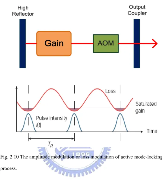
Fig. 2.10 The amplitude modulation or loss modulation of active mode-locking process.

We usually introduce the amplitude modulator such as acousto-optic modulator and electro-optic modulator into the cavity which periodically varies the intracavity loss. All the lights in the cavity will experience a net loss larger than the net gain, which block the lasing mechanism, except those which pass through the modulator around the lowest loss point, which will generate the laser pulse at this moment. The modulation period has to be matched to the cavity round-trip time, and then the laser beam which is incident at particular point in the modulation cycle will be incident at the same point after one round trip of the cavity so that the phase of each lasing mode will be fixed. Fig. 2.10 shows the amplitude modulation or loss modulation of active mode-locking process in the time domain.

(37)

As mentioned in the theory of mode locking, a laser consist of a gain medium inside two reflected mirrors and the distance between the two reflected mirrors which is the cavity round trip will decide the longitudinal modes separated in frequency by ωc= 2π(c/2d)=2π/τRT,

where τRT is the round-trip time. If the gain is larger than the loss for these longitudinal

modes, these longitudinal modes will all be lasing. But the phase between these longitudinal modes is random and not related to each other. Placing the amplitude modulator near one of the mirrors, and a cosinusoidal signal of the modulation at the frequency Ω=Nωc will be used

to generates sidebands at ω0±Ω, which the frequency of the central mode is ω0. These

matched modes lasing in the same round trip cycle will have the fixed phase condition so that they will interference to each other to generate an extremely giant and short pulse.

Now we consider the mathematical theory of amplitude modulation. The signal of the amplitude modulation can be written as q(t) = M (1 − cos(Ωt)) where M is the modulation index. The mode-locked lasers by amplitude modulation can be written as the master equation. 2 2

[ ( )

(1 cos(

))]

R g M

A

T

g T

D

l

M

t

A

T

t

ω

∂

=

+

− −

−

⋅

∂

(2.31)

Where we define A is a slowly varying field envelope, that is already normalized to the total power flow in the beam, TR =2L/Vg,0 is dispersion coefficients per resonator round-trip, g(T)

is the gain and Dg is the curvature of the gain at the maximum of the Lorentzian lineshape (is

also the gain dispersion).

The first and second terms of the Master equation are the interaction by gain. The third and fourth terms of the equation are the interaction by loss and modulator. We fix the gain in Eq. at its stationary value because it might be constant in time domain, and the equation can be solved by separation of variables. The pulses will have a width much shorter than the round-trip time TR, and they will be located in the minimum of the amplitude modulation where the cosine-function can be approximated by a parabola function and the equation will

(38)

become a linear P.D.E. The differential equation corresponds to the Schrödinger-Operator of the harmonic oscillator problem. Therefore, we can calculate the eigen functions of this operator which are the Hermite-Gaussians

( , )

( )

nT T/ R n n

A T t

=

A t e

λ (2.32) 2 2 2

( )

( / )

2 !

a t n n _n n a a

W

A t

H t

e

n

τ

π τ

−

=

where τa defines the width of the Gaussian.

Thus active mode-locking without detuning between resonator round-trip time and modulator period leads to Gaussian steady state pulses with a FWHM pulse width

∆

t

_FWHM

=

2 (2 ) 1.66

In

τ

_a

=

τ

_a (2.33) And the spectrum of the Gaussian pulse is obtained by

2 ( ) 2 0

( )

0

( )

a i t n a

A

A t e dt

W

e

ωτ ω

ω

=

∫

_−∞∞

=

π

τ

− (2.34) where its FWHM in frequency domain is

1.66

2

FWHM a

f

πτ

∆

=

(2.35)

Therefore, the time-bandwidth product of the Gaussian pulse is

∆

t

_FWHM

⋅ ∆

f

_FWHM

=

0.44

(2.36) The stationary pulse of the mode-locked laser is achieved when two effects which the generation of the pulse are due to the parabolic amplitude modulation in the time domain and the parabolic filtering due to the gain in the frequency domain corresponding to pulse shortening and pulse stretching balance. Actively mode-locking typically by amplitude modulation only results in pulse width in the range of several tens picoseconds because the pulse width does only scale with the inverse square root of the gain bandwidth and external modulation is limited to electronic speed.

(39)

In the frequency domain, the amplitude modulator transfers energy from each mode to its neighboring mode. In other words, it redistributes energy from the center mode to the wings of the spectrum. This process seeds and injection will lock neighboring modes. We can see the phenomenon of neighboring modes locking from the below equation which is the fourth term of above master equation

0

0 0 0

0 0 1 0 1

[1 cos(

)]exp(

)

1

1 [exp(

)

exp( (

))

exp( (

))]

2

1

1 [ exp(

)

exp(

)

exp(

)]

2

M n n n M n M n n n

M

t

j

t

M

j

t

j

t

j

t

M

j

t

j

t

j

t

ω

₋

ω

₊

−

= −

−

+

=

−

+

(2.37) So as we have mentioned before, if the modulation frequency is the same or integer times to the cavity round-trip frequency. The sidebands generated from each running mode are injected into the neighboring modes which lead to synchronization and locking of neighboring modes, i.e. mode-locking.

(40)

References

[2.1] Joseph T. Verdeyen, “Laser Electronics,” third edition, Prentice Hall Englewood Cliffs, New Jersey 07632

[2.2] Amnon Yariv, Pochi Yen, “Photonics,” sixth edition, New York Oxford university press 2007.

[2.3] B. E. A. Saleh and M. C. Teich, “Fundamentals of Photonics,” John Wiley & Sons, New York _1991_.

[2.4] Y. Wang and Chang-Quing Xu, “Actively Q-switched fiber lasers: Switching dynamics and nonlinear processes,” Progress in Quantum Electronics 31, 131–216 (2007)

[2.5] Y. Wang, A. Martinez-Rios and Hong Po, “Analysis of a Q-switched ytterbium-doped double-clad fiber laser with simultaneous mode locking,” Opt. Commun. 224, 113-123 (2003).

[2.6] P. K. Das, C. M. DeCusatis, “Acoustio-Optic Signal Processing: Fundamentals& Applications,” Artech House, Boston‧London.

[2.7] Herman A. Haus, “Mode-locking of Lasers”, IEEE J.on Selected topics in Quant. Electron. 6, 1773(2000)

[2.8] Dirk J. Kuizenga and A. E. Siegman, “FM and AM mode locking of the homogeneous laser-Part I:Theory” IEEE J. Quantum Electronics, vol. 6, no. 11, pp. 694-708 (1970)

(41)

Chapter 3 Experimental results

3.1 Q-switched pulse generation

3.1-1 Experimental setup

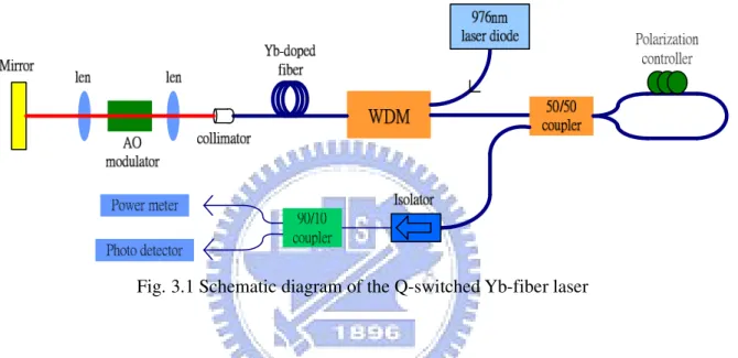
Fig. 3.1 Schematic diagram of the Q-switched Yb-fiber laser

The schematic setup of Q-switched pulses generation from our ytterbium doped fiber laser with a linear cavity configuration is shown in Fig. 3.1. A laser diode with 976 nm center wavelength is used to pump 0.2 m long Yb-doped fiber (mode-field diameter 4.4 µm, 1200 dB/m absorption @ 976 nm) through a wavelength-division multiplexing (WDM) coupler. A fiber loop, including a 50/50 coupler and a polarization controller with total length of 365 cm, is used as the output coupler. In the other end, a collimator is used to collimate the laser beam from fiber to the free space. Then, a focal lens with 50 mm focal length is used to focus the beam onto an acousto-optic modulator (Neos inc. 40 MHz RF)to

produce the Q-switching operation. The zeroth order diffraction beam from the acousto-optic modulator is used to resonate in the cavity for Q-switching. A re-imaging lens with the same focus lens is used to re-image the beam on a high reflective mirror as the

(42)

other end mirror. An isolator outside the output coupler is used to prevent the feedback of the output light into the laser cavity. Finally, we use a 90/10 coupler to divide the light into the power meter (Newport inc.), oscilloscope (Wave Surfer 62 Xs, bandwidth 650 MHz, LeCroy) and optical spectrum analyzer (AQ6315A, Ando inc.) for monitoring the state of laser.

3.1-2 R

esults and discussions

The Q-switched operation of the laser can be achieved by increasing the pump power above 73 mW, but the periods of Q-switched pulses are irregular. The regular operation of Q-switched pulse can be obtained by further increasing the pump power. Fig. 3.2 shows the time traces of stable Q-switched pulses on the oscilloscope with 120 kHz modulation frequency and 300mW pump power. A number of discrete and periodic Q-switched pulses with time period about 8.4 µs can be seen in Fig. 3.2. The time period corresponds to the external modulation frequency of the AOM at 120 kHz. The period of the pulse train is almost regular as well as its amplitude fluctuation is reasonably small for all peaks as shown in Fig. 3.2.

Fig. 3.2 Time traces of Q-switched pulse trains at 120 kHz modulation frequency and the 300 mW pump power.

0 20 40 60 80 100 In te n s it y ( A .U .) Time (µµµµs)

(43)

When we change the modulation frequency of the AOM, the satellite pulses of Q-switched pulses can be seen on the time traces of the oscilloscope. Fig. 3.3 (a)-(c) shows the time traces of Q-switched pulses on the oscilloscope at the pump power of 300 mW by setting the AOM modulation frequency at 40 kHz, 70 kHz, 100 kHz. At lower modulation frequencies, the satellite pulses generate after the main pulse. In addition, the number of satellite pulses will also increase as modulation frequencies decrease. There are 3 satellite pulses behind the main pulse at 40 kHz modulation frequency. And only one satellite pulse appears at 70 kHz modulation frequency. The satellite pulses almost disappeared on the oscilloscope when we increase the modulation frequency to be at 100 kHz.

Fig. 3.3 Time traces of Q-switched pulse trains at (a) 40 kHz (b) 70 kHz (c) 100 kHz.

0 2 5

5 0

7 5

In

te

n

s

it

y

(

A.

U. )

T i m e (

µµµµ

s )

( a )

0 2 5

5 0

7 5

( c )

( b )

T i m e (

µµµµ

s )

0 2 5

5 0

7 5 1 0 0

T i m e (

µµµµ

s )

(44)

Fig. 3.4 The formation of satellite pulses at long switch off time duration.

The satellite pulses are produced by the mechanism illustrated in Fig. 3.4. After the main Q-switch pulse is generated, the population inversion is consumed such that the gain is smaller than loss inside the cavity. At the moment, the pump power is continuously injected into the cavity, which will cause the gain to become lager than the loss again. As the gain is lager than the loss, the satellite pulse is generated. When the AO modulation frequency is lower (that is to say, the time duration for one period is longer) or the pump power is higher, the satellite pulses are more easily generated and their number will also be greater. These predictions from the Q-switch theory match the observations in our experiment.

(45)

Summary of this section

In this section, we observe the stable Q-switching generation by using an AO modulator in our scheme. The time traces of stable Q-switched pulses can be observed on the oscilloscope at the modulation frequency around 120 kHz and the pump power of 300mW. By lowering the AOM modulation frequencies, the satellite pulses appear after the main pulse with the same pump power. The number of satellite pulses will also increase at lower modulation frequencies.

(46)

3.2 Q-switched mode-locked pulse generation

In the previous work, the generation of stable Q-switched pulses by using an AO modulator has been successful demonstrated. In the literature, for diode pump Nd:YVO4 lasers and

Er-doped fiber laser, the stable QML operation has been demonstrated by using an AO modulator [3.1,3.2]. In their work, the AOM play both roles as the Q-switcher and the mode-locker. Therefore in this section, we want to study whether the Q-switched mode-locked pulses can also be generated in our Yb-doped fiber laser by the AO modulator.

3.2-1 Experimental setup

Fig. 3.5 Schematic diagram of the Q-switched mode-locked ytterbium fiber laser.

In order to simultaneously generate the Q-switched and mode-locked pulses, we make some minor modifications in our laser setup as shown in Fig. 3.5. Only one focal lens with 7.5 cm focal length outside the collimator is used to focus the beam on the AOM. The distance between the collimator and the focal lens is about 13 cm, and the distance between the focal lens and the end mirror is about 8 cm. Similarly, the AOM is placed in front of

50/50 coupler WDM Polarization controller 976nm laser diode AO modulator

Mirror _len Yb-doped _fiber

90/10 coupler Photo detector Power meter collimator Isolator

(47)

the end mirror closely to make the laser beam size on the AOM as small as possible with a tiny deflection angle by carefully adjusting the position of the AOM and end mirror. Here the first order diffraction beam from acousto-optic modulator is used to resonate in the cavity for Q-switching and mode-locking operation. In the same way, the 976 nm pump laser diodes are used to pump 0.2 m long Yb-doped fiber through a WDM coupler. A fiber loop, including a 50/50 coupler and a polarization controller with total length 365 cm, is used as the output coupler. An isolator and a 90/10 coupler are connected to the output coupler to divide the light into the power meter, oscilloscope and optical spectrum analyzer for monitoring the state of the laser.

3.2-2 R

esults and discussions

In this configuration, the simultaneously Q-switched and mode-locked operation of the laser can be achieved by increasing the pump power above 80 mW. Similarly, the time period of Q-switched envelope is not regular and the pulses have relative large amplitude fluctuations. The stable QML output pulses with regular time period can be seen when the pump power is above 100 mW. Fig. 3.6 shows the time traces of stable Q-switched mode-locked pulses on the oscilloscope with modulation frequency around 100 kHz and the pump power of 188 mW. In terms of Q-switched envelope trains, the repetition rate is almost regular about 100 kHz and the fluctuations are relatively small. By expanding the Q-switched envelopes in time domain, we can see that there are evident mode-locked pulse trains inside every Q-switched envelope. Fig. 3.6 (b) reveals the expanded single Q-switching envelope, in which a number of discrete and periodic mode-locked pulses with time period about 25 ns (corresponding to the repetition rate of 40 MHz) can be obviously seen. The corresponding optical spectrum shown in the inset of Fig. 3.6 (a) indicates that the center wavelength is 1025 nm and the bandwidth is about 3.68 nm. The shape of the optical