Parametric Searching Algorithms with Adaptive
Strategy for Three Dimensional Protein Structures
Alignments
Hsiang-Sheng Shin
Shih-Peng Huang
Yaw-Ling Lin
∗Department of Comput. Sci. and Info. Management, Providence University,
200 Chung Chi Road, Shalu, Taichung County, Taiwan 433.
[email protected], [email protected],[email protected]
Abstract
Protein structure provides the opportunity to rec-ognize homology that is undetectable by sequence comparison, and it represents a powerful means of discovering functions, yielding direct insight into the molecular mechanisms.
Currently, there are several techniques avail-able in attempting to find the optimal alignment of shared structural motifs between two proteins.
In this paper, we show the effectiveness of the proposed refinement methods [11] by a set of ex-periments, which have improved some previous re-sults. We propose a better adaptive strategy to have better parameters, and we can get a better pairwise alignments of protein structures. We can apply this strategy to find more accurate and sim-ilar protein structure pairings.
Keywords: structural proteomics, alignments and comparisons, refinement, pretest algorithm
1
Introduction
Protein structures play a critical role in vital biological functions [7]. There are more and more protein structures determined by the advances in X-ray crystallography and NMR spectroscopy. Therefore, more and more people want to analyze and classify these protein structures in order to understand their relationships with protein func-tions [6].
Protein structures determine the protein func-tion, we are now trying to chase down all possible relationship about human and all kinds of pro-teins. According to this reason, the comparisons
∗Corresponding author. This work is supported by
grants from the Taichung Veterans General Hospital and Providence University (TCVGH-PU-968110) and in part by the National Science Council (NSC-96-2221-E-126-002) Taichung, Taiwan, Republic of China.
of protein structures come into existence, and some academics proposed some methods to com-pare protein structures such as DALI [9],VAST [15] and CE [21]. All of them can find the simi-larity score between two or more structures. Their structural alignments are a form of sequence align-ment based on comparison of three-dimensional conformation. But they can only find the struc-tural alignments with sequencing. Lin publishes another methods to compare proteins in terms of three dimensional protein structure alignments [14]. We can have better score by Lin’s methods if we use the VAST alignment to be its initial align-ment [11].
One of the primary goals of structural alignment programs is to quantitatively measure the level of structural similarity between all pairs of known protein structures. This data can provide sev-eral meaningful insights into the nature of protein structures and their functional mechanisms. The three dimensional structure of proteins is highly conserved during evolution [4]. Protein are con-structed by one or more polypeptide chains that fold into complicated 3D structures.
Detection of proteins with a similar fold can suggest a common ancestor, and often a similar function [5]. Comparison of 3D structures makes it possible to establish distant relationships, even between protein families distinct in terms of se-quence comparison alone. This is why structural alignment of proteins increases our understanding of more distant evolutionary relationships [3, 12]. The link between structural classification and se-quence families enables us to study functions of various folds, or whole proteins [14].
In this paper, first we introduce the pro-cess about why we develop the three parameters searching programs and what is the tools to com-pare protein structures in the literatures. Sec-ondly, we explain about how to develop our
meth-ods and what our methmeth-ods are. In the third
pro-posed methods and the CE methods and then show the experimental results. In the third, we use a adaptive strategy to find the initial space without any suggestion and compare them with VAST and CE.
2
Previous Work
In this section, we introduce rmsd which is the standard of measure for structural comparison, and then according to the rmsd we can find the key point, rotation matrix, which can rotate the 3D protein coordinates to the better place. Then, we can be easy to compare the rmsd between the rotated protein and the other protein. We can find the other critical analysis by Euler’s rota-tion theorem [13], and we can use the three an-gles to stand for the rotation. But our methods are not the same as Euler’s theorem. We become deformed the Euler’s theorem and find another adaptable three angles for our programs. We point out the two important concepts. One is the rota-tion matrix, and another is the Minimum Bipar-tite Matching. Our previous programs integrate the two important components to compare protein structures. The algorithm is showed in figure 1.
2.1
Root mean squared deviation
The smallest root mean squared deviation
(rmsd) is a least-squares fitting method for two
sequences of points [10]. The idea is to align atom vectors of the two given (molecular) structures, and use the common least averaged squared errors as a measurement of differences between these two
(paired) sequences. Formally, let P = hp1, . . . , pni
and Q = hq1, . . . , qni be two sequences of points.
We assume that P is translated so that its centroid (1
n
Pn
k=1pk) is at the origin. We also assume that
Q is translated in the same way. For each point
or vector x, let (x)i(i = 1, 2, 3) denote the i-th
(X, Y, Z) coordinate value of x, and kxk denote the length of x. Let
rmsd(P, Q, R, a) = v u u t 1 n n X k=1 kRpk+ a − qkk2, (1) where R is a rotation matrix and a is a translation vector. Then, the rmsd value d(P, Q) between P
and Q is defined by d(P, Q) = minR,ad(P, Q, R, a).
Although complicated as it might appear, the op-timal rotation matrix and translation vector can be found simultaneously in O(n) time. Schwartz [20] showed that d(P, Q, R, a) is minimized when a = 0 and
R = (AtA)1
2A−1, (2)
where the matrix A = (Aij) i, j = 1, 2, 3 is given
by Aij = n X k=1 (pk)i(qk)j, (3)
where A12 = B means BB = A , and o denotes
the zero vector. Thus, d(P, Q), R and a can be computed in O(n) time [17].
We adopt Martin’s ProFit package (standing for protein fitting system) [16] to calculate the rmsd between C-α atoms of paired protein backbones. ProFit has many features including flexible spec-ification of fitting zones and atoms, calculation of RMS over different zones or atoms, RMS-by-residue calculation. Fitting was performed using the McLachlan algorithm [17].
2.2
Euler’s Rotation Theorem
According to Euler’s rotation theorem [13] , any rotation can about the origin point be described by using three angles. The rotation is determined by 3 consecutive rotations with 3 Euler angles
(θ, β0, γ0). The first rotation is done by the angle θ
(= sin−1α) around the z-axis, the second is done
by the angle β0(= βπ) around the x-axis, and the
third rotation is done by the angle γ0 around the
z-axis.
As a result, we reduce the problem of finding a good rotation matrix to the new problem of find-ing a good 3-parameter. The rotation matrix is thus characterized by just adjusting the 3 uni-formly distributed parameters.
2.3
Our Rotation Matrix
our 3-parameter method (α, β, γ) can be sum-marized as the following:
• Rotation around x-axis:
Given a unit vector p = (x, y, z)T, p is
trans-formed into p0by a rotation around the x-axis
by angle sin−1α = θ. That is, let
p0= xyαα zα = 10 √1 − α0 2 −α0 0 α √1 − α2 ·p
Since sin θ = α and thus, cos θ =√1 − α2.
• Rotation around z-axis:
The vector, p0= (x
α, yα, zα)T, is transformed
into the probe p00by a rotation around the
z-axis by angle βπ. That is, let
p00= xyββ zβ =
cos βπ − sin βπ 0sin βπ cos βπ 0
0 0 1
·p0
then we will get new coordinate of
Struc-Align(P, Q, αI, βI, γI, p)
Input: Two set of 3D coordinates of points P = {p1, p2, . . . , pn} and Q = {q1, q2, . . . , qm} ; n < m.
The αI , βI and γI are real numbers that are between -1 to 1.
B These inputs control the initial position of 3 parameters box and affect the explored area.
B p is the vector (x, y, z)T, explained in section 2.1.
Output: (s, α, β, γ) is a sufficiently low Rmsd s and (α, β, γ).
B (α, β, γ) is the best position of 3 parameters box.
Global : T, t, F, αmax, βmax, γmax.
The threshold T and F are both integer numbers. B T is total trial number of perturbation.
B t is the count that records the number of perturbation carried out so far.
B F is the maximum number of consecutive failed perturbations for a probe to restart.
αmax, βmax, γmax are real numbers between 0 to 1.
B These inputs control the range of parameters perturbation variances.
1 (α, β, γ) ← (αs, βs, γs) ← (αI, βI, γI).
2 Q0← Trans(Q,Rot-m(α, β, γ, p)). B Q0 is a temp array of atoms set of protein.
3 L ← Mbm(P, Q0) ; (R, a) ←Ms-Fit(L, P, Q0) ; s ←Rmsd(P, Q0, R, a).
4 f ← 0. B Initializing the counter.
5 while t ≤ T do
6 (α0, β0, γ0) ←Perturb(α, β, γ).
7 Q0 ← Trans(Q,Rot-m(α0, β0, γ0, p)). B Q0 is a temp array of atoms set of protein.
8 L ← Mbm(P, Q0) ; (R, a) ←Ms-Fit(L, P, Q0) ; s0 ←Rmsd(P, Q0, R, a). 9 if s0 ≤ s then s ← s0;(α, β, γ) ← (α s, βs, γs) ← (α0, β0, γ0) ; f ← 0 ; 10 else f ← f +1. 11 if f ≥ F then return (s, αs, βs, γs). 12 t ← t+1. 13 return (s, αs, βs, γs).
Mbm(P, Q) returns the minimum bipartite matching of two point sets P and Q.
Perturb(α, β, γ).
Input: The α,β and γ are real numbers between -1 to 1.
B These inputs control the present position of 3 parameters box and affect the explore area.
Output: 3 real numbers (α0, β0, γ0).
B These outputs are the new position of 3 parameters box.
1 ∆α ←Rand(−αmax, αmax) ; ∆β ←Rand(−βmax, βmax) ; ∆γ ←Rand(−γmax, γmax).
2 α0←Back(α + ∆α) ; β0←Round(β + ∆β) ; γ0 ←Round(γ + ∆γ).
3 return (α0, β0, γ0).
Rand(a, b) is a random function returning a real number uniformly distributed between a and b.
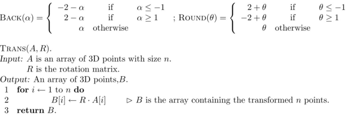
Back(α) = −2 − α if α ≤ −1 2 − α if α ≥ 1 α otherwise ; Round(θ) = 2 + θ if θ ≤ −1 −2 + θ if θ ≥ 1 θ otherwise Trans(A, R).
Input: A is an array of 3D points with size n. R is the rotation matrix.
Output: An array of 3D points,B.
1 for i ← 1 to n do
2 B[i] ← R · A[i] B B is the array containing the transformed n points. 3 return B.
Figure 1: Aligning two sets of atoms with low rmsd by pairing points according to the minimum bipartite matching measurement
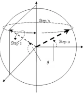
Figure 2: Three parameters (α, β, γ), or angles (sin−1α, βπ, γπ), suffice to determine a rigid 3D rotation
of points about origin.
• Rotation around the probe p00:
The last rotation matrix, Rγ, do the body
ro-tation around the probe p00 by angle γπ; see
[8] for related discussions about the transfor-mation. That is, let
(x, y, z) = (xβ, yβ, zβ)T. c = cos γπ, s = sin γπ, h = 1 − c. Rγ = c + x 2h xyh − zs xzh + ys xyh + zs c + y2h yzh − xs xzh − ys yzh + xs c − z2h
2.4
Minimum Bipartite Matching
There are several proposed algorithms for the minimum bipartite matching problem; sometimes it is also referred as the assignment problem. Here we adopted the Munkres [18, 2, 1, 19] algorithm. The public available implementation is written with Perl language. To improve the efficiency of computation, we implement the Munkres algo-rithm and write hundreds lines of C Codes, and and the produced codes are strictly verified by comparing the results with the public Perl pack-age.
2.5
Perturb
Note that the methodology of the current sys-tem is generally a randomized algorithm and a variable, Perturb algorithm and F . The per-formance of Perturb algorithm is depended on various setting of 3-parameter, αmax, βmax, γmax.
The perturb algorithm is displayed in figure 1.
3
The Experiment for Three
Pa-rameters
In order to obtain the suitable 3-parameters, we select 50 samples of 6,000 samples, and carry fol-lowing experiments to find out good parameters of the our programs.
The experiments can help us to analyze how the 3-parameter, αmax, βmax, γmax, affects the
fi-nal rmsd. The better αmax, βmax, and γmax
are found. We have to assume that T is 50, and F is 11. The other two parameters of 3-parameters have to be set to 0.2. For example, if we want to search a good αmax, we must set
βmax= γmax= 0.2 and so on.
Then, We start to performance the experiment. First, we test a good αmaxamong 0.2, 0.4, 0.6, 0.8,
and 1. Secondly, we use uniformly distributed method to divide the two neighbors of the maxi-mal result into six number and test the six num-bers. For example, the maximum result is 0.4, and its neighbors are 0.2 and 0.6. We have to test 0.25, 0.3, 0.35, 0.45, 0.5, and 0.55. Thirdly, in last step we can find another maximal result from the six value. We use uniformly distributed method to divide the two neighbors of the max-imal result into two numbers. For example, if the maximal result is 0.45, we can get 0.425 and 0.475. Last of all, we test the two value and choose maximal result for our final parameter. Af-ter these experiments we find a good 3-parameAf-ter, (αmax, βmax, γmax) = (0.475, 0.2, 0.2), and the
re-sults are shown in Figure 3 and Figure 4.
Furthermore, we have another experiment. We try to analyze how the variable, F , affects the final
rmsd. We set T = 50, and then we test F between
1 2
√
T and 2√T by experience. Now F which we
test is from 3 to 15. Under the good 3-parameters, (αmax, βmax, γmax) = (0.475, 0.2, 0.2), we find
that the good value of F is 13 and the results are shown in Figure 4.
4
The Pretest Algorithm
The main idea for the pretest algorithm is to save the computer times in the finite resource. We have only finite resource to get the best effect. Therefore, we develop the Pretest Algorithm. The main concept of pretest algorithm is to filter the fitting parameters for our programs. We can use the algorithm to find a initial alignment from the
1.1 1.2 1.3 1.4 1.5 1.6 1.7 0.2 0.3 0.4 0.5 0.6 0.7 0.8 0.9 1
The improvement ratio (%)
The variance 0.7 0.8 0.9 1 1.1 1.2 1.3 1.4 1.5 1.6 0.1 0.2 0.3 0.4 0.5 0.6 0.7 0.8 0.9 1
The improvement ratio (%)
The variance
Figure 3: The Experimental improvement ratios under different αmax and βmax, and fix the other
pa-rameters. 0.6 0.8 1 1.2 1.4 1.6 0.1 0.2 0.3 0.4 0.5 0.6 0.7 0.8 0.9 1
The improvement ratio (%)
The variance 1 1.1 1.2 1.3 1.4 1.5 1.6 1.7 1.8 3 4 5 6 7 8 9 10 11 12 13 14 15
The improvement ratio (%)
The variance
Figure 4: The Experimental improvement ratios under different γmaxand F , and fix the other parameters.
Align-TOR-K(P, Q, T, F, αmax, βmax, γmax, T OR, K)
Input: The (P, Q, T, F, αmax, βmax, γmax) parameters are explained in figure 1.
T OR is a real number representing the rmsd threshold for the pretesting phase. K is a integer that control the maximum number of failed perturbations. Output: (s, L)
1 s ← ∞ ; p ← (0, 1, 0)T.
2 while t ≤ T do
3 α ← Rand(−1, 1) ; β ← Rand(−1, 1) ; γ ← Rand(−1, 1) ; k ← 0.
4 B (α, β, γ) are uniformly distributed random values ranged in (−1, 1). 5 while k ≤ K do
6 (α0, β0, γ0) ←Perturb(α, β, γ).
7 Q0← Trans(Q,Rot-m(α0, β0, γ0, p)). B Q0is a temp array of atoms set of protein.
8 L ← Mbm(P, Q0) ; (R, a) ←Ms-Fit(L, P, Q0) ; s0←Rmsd(P, Q0, R, a). 9 if s0≤ T OR · s then (s0, α0 s, βs0, γs0) ←Struc-Align(P, Q, α, β, γ, p) ; k ← K. 10 k ← k + 1 ; t ← t + 1. 11 if s0≤ s then s ← s0; (α s, βs, γs) ← (α0s, βs0, γs0). 12 Q0← Trans(Q,Rot-m(α
s, βs, γs, p)). B Q0is a temp array of atoms set of protein.
13 L ← Mbm(P, Q0). B L is the matching list of point sets P and Q.
14 return (s, L).
Figure 5: The pretest algorithm can try to filter the fitting parameters for our programs. We can use the algorithm to find a initial alignment for protein pairings.
protein pairings, and we use two thresholds, TOR and K, to filter the possible candidate parame-ters. TOR is a real number to represent the rmsd threshold for the pretesting phase. K is a integer that control the maximum number of failed per-turbations. We give the program K times to find a RMSD value which must satisfy the following condition
s0/s ≤ T OR
, where s is the minimal rmsd which we find in this time and s’ is the value which we find under the k times testing. If the s’ is ok, we use this parameters to run our program and give it more resource to find a better result. By the way, we can save a lot of resources to find a good alignment.
5
Experimental Result
In this section, we show the experimental meth-ods and result between CE methmeth-ods and our previ-ous methods. First of all, we illustrate what sam-ples we use for our experiments, and then we ex-plain that the samples in VAST are different from the one in CE. Secondly, we analyze the improve-ment ratios of our method tested on the given data. In the third part, we display and analyze the experimental results about our Pretest algo-rithms, CE and VAST. Finally, we analyze the experimental execution time of our programs for some different conditions.
5.1
Sample Source
In our previous experiment, We choose the PDB for our experimental sample source, and we ran-domly pick 200 protein structures in the PDB database as our experimental subjects by the uni-form distribution sampling. For each chosen pro-tein structures We randomly choose 30 structure alignments listed on the database of VAST as the tested targets. Totally, there are 6,000 protein pairings tested by our previous experiment. We use the term, PA, to stand for one of the 200 ran-domly picked protein structures, and we use PB to stand for one of the 30 neighbors of each PA. we randomly get the three parameters for our meth-ods to compare with the VAST methmeth-ods. The sample distribution is showed in Figure 6. We illustrate the number of C-α atoms of PA, the number of protein pairings and the average of im-proved ratio, at Figure 7. The result which we improve against the VAST is 9.29%.
We want to use the same samples to test the CE method. But we find that the alignments sought out by CE are different from the ones by VAST. The CE programs always find out its own alignments, and we can not assign the number of
C-α for our experiments. In this situation, the VAST and the CE can not be compared for each other. Therefore, we can only compare the re-sults between our methods and the CE methods. We divide the process which we get the new pro-tein pairings into several parts. First, we use the 6,000 protein pairings from VAST for our origi-nal samples. We input each pairings into the CE programs, and the new protein pairings are out-putted. We use the aligned atoms from PA we input for our new PA, and the PB is the same as which we input. We call the new PA, ce-PA. We use the pairings of ce-PA and PB for our new sam-ple pairings. The relation between the number of C-α atoms of ce-PA and the number of protein pairs are illustrated at Figure 8.
5.2
The Experimental Result With
CE
Now we have 6,000 new protein pairings for our experiment. We use the better three parameter, (0.475, 0.2, 0.2), to execute the Struc-align al-gorithm. We first measures each sample pairings by calculating its original alignment’s rmsd value. The measurement is confirmed and double checked wich the rmsd by the PROFIT package kits [16].
After we finish the 6,000 samples, the results note that we can improves almost every sampled CE pairs. By the ascending order on the number of C-α atoms of ce-PA, we partition the samples into 40 points, with each point standing for 150 protein pairs. Figure 9 shows the relation between the number of C-α atoms of PA and the improve-ment ratios contrast to the given VAST alignimprove-ment. The formula of the improvement ratio is defined by
ρ = (A − B)/A,
where A is the original rmsd value by the CE align-ment, while B is improved(smaller) rmsd value by our structure alignment method. The improve-ment ratios of our samples are mostly distributed from 8% to 15%. As a total, the average of the improvement ratios is 11.03%.
The execution time of the experiment for our method is summarized in Figure 10, which shows the relation between the number of C-α atoms of ce-PA and the execution time (CPU processor time) of our structure alignment system needed for the samples to run. Note that each drawn point in Figure 10 represents a group of 150 protein pairs. The structure alignment system is implemented and tested under the Linux Red Hat 4.0 system. Each of the experimental machine is equipped with Intel(R) Pentium(R) 4 CPU 3.00GHz pro-cessor and 2GB RAM main memory. The experi-ment takes approximately 100 hours to finish the experiment on the total 6,000 protein structure
0 100 200 300 400 500 600 400> 350 300 250 200 150 100 50 0
The number of protein pairings
The number of C-alpha atoms of PA
Figure 6: The distribution of the 200 randomly picked protein structures in PDB and their 30 neighbor structures. The total number of protein pairs is 6,000.
The number The number The average The average The standard The standard
of C-α of protein of improved of execution deviation of deviation of
atoms of PA pairings ratio (%) time (Sec) improved ratio (%) execution time (Sec)
50< 1541 7.61 0.57 11.99 1.27 50-100 1586 7.17 5.98 11.98 5.54 100-150 1030 8.42 15.16 12.48 14.83 150-200 674 14.71 41.73 15.61 41.49 200-250 469 11.30 161.01 14.74 160.92 250-300 404 9.57 401.65 15.07 401.90 300-350 186 17.57 873.34 18.21 875.59 350-400 40 12.66 1592.63 25.30 1612.83 400> 70 15.67 10315.05 21.41 10389.45 Total 6000 9.29 206.68 13.22 206.26
Figure 7: The result is to execute the previous algorithm with random parameters and compare with the VAST. The distribution of our experimental data containing the number of C-α atoms of PA, the number of protein pairings, the average of improved ratio, the average of execution time,the standard deviation of improved ratio and the standard deviation of execution time.
0 100 200 300 400 500 600 370> 350 300 250 200 150 100 50 0
The number of protein pairings
The number of C-alpha atoms of ce-PA
2 4 6 8 10 12 14 16 18 20 0 100 200 300 400 500
The improvement ratios (%)
The number of C-alpha atoms of ce-PA
The average of improved ratio : 11.03%
Figure 9: The improvement ratios opposite to the
rmsd of the CE alignment. The improvement ratios
are mostly distributed from 8% to 15%. The average is 11.03%. Each point stands for 150 sample pairings.
0 200 400 600 800 1000 1200 1400 50 100 150 200 250 300 350 400
The executtion time(Sec)
The number of C-alpha atoms of ce-PA
Figure 10: The execution time of our structure align-ment system with better parameters needed for the samples to run. Each point stands for 150 sample pairings.
pairings. The Figure 11 is the result which we compare against the CE, and the average of im-proved ratio is 11.03%.
5.3
The Experimental Result With
CE for Pretest Algorithm
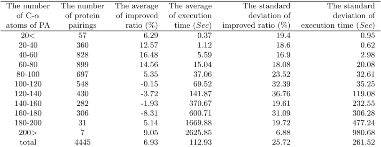
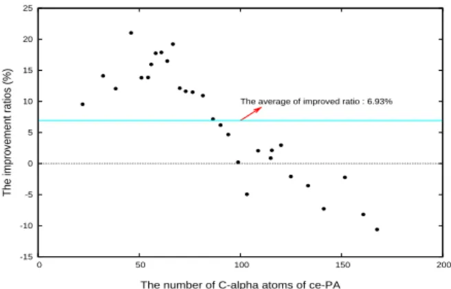
We execute the pretest algorithm for our exper-iment.First, we have to set the other parameters. The parameters for us to execute this experiment is T = 330, F = 8, α = 0.35, β = 0.1, γ = 0.18. We give the TOR for 1.23 and the K for 1 to run the 6,000 data. We also use the same ce-PA to run the program. Our program can find a alignment. We compared the value of RMSD between our align-ment and the CE alignalign-ment. In this comparison, our program is 6.93% more than the CE. The exe-cution time for the program is shoed in Figure 14. We have finished the 4,445 protein pairings, but the time we have to spend on the other 1,555 is for a long time. To date, we continue to run them. The distribution for the improvement ratio is showed in Figure 13. When the number of atom for ce-PA is less than 100, we almost find a better alignment than the CE. But the result is not good if the ce-PA is more than 100. This experiment can indicate that we can find a better value about TOR and K to have better alignment. The im-provement ratios opposite to the rmsd of the CE alignment. The improvement ratios are mostly greater than 0. The average is 6.93%. The execu-tion time for the program is shoed in Figure 14. The experimental result is showed in Figure 12.
6
Conclusion and Future Work
Bioinformatics has become an essential tool not only to basic research but also to serious research
in biotechnology and biomedical sciences. Cur-rently, the field is under enormous expansion and witnessed by the dramatic increase in the number of related bioinformatic literatures.
In this paper, we use the algorithms which we proposed previous to improve the rmsd value be-tween protein structure pairings by finding better alignment list. We use a set of experiments to test the parameters. We apply the tested param-eters to run the experiment results. Our method with better parameters can improves the align-ment computed by the CE package and the aver-age of improvement ratios is 11.03%. Therefore, the system demonstrates that the method with 3D Euclidean distance, minimum bipartite match-ing and perturbed parametric searchmatch-ing scheme indeed improves existed known system like the VAST and the CE. It is interesting to know what is the best parameter for our method. We can use another better one to find them.
We use the pretest algorithm to test the protein pairings without initial alignment. We can find the better alignments than the CE. We can have another better method to find the initial align-ment for the global alignalign-ments. The average which our result can have is 6.93% more than the result of CE. Our methods need the better parameters to have the better results. We can continue to test them. Besides, we can use our program to classify the protein and fine the similarity about all proteins.
Furthermore, since the structure compari-son problem, like many scientific computa-tion/simulation problem, is very time-consuming under cases of large structures and large num-ber of paired structures, it is desirable to imple-ment the system under massive parallel machines cluster, e.g., the grid-environment, to increase the throughput of the system.
The number The number The average The average The standard The standard
of C-α of protein of improved of execution deviation of deviation of
atoms of PA pairings ratio (%) time (Sec) improved ratio (%) execution time (Sec)
50< 682 12.23 0.10 10.41 0.09 50-100 2208 14.18 1.01 9.61 0.68 100-150 1150 9.50 5.50 7.13 2.98 150-200 768 8.55 20.79 7.22 9.51 200-250 489 8.16 50.19 6.77 13.99 250-300 450 7.62 96.73 7.31 39.29 300-350 160 7.40 220.59 7.74 61.52 350-400 31 4.55 349.58 4.46 54.06 400> 62 5.02 2772.87 3.58 1602.22 Total 6000 11.03 51.79 8.93 325.64
Figure 11: The result is to execute the previous algorithm with tested parameters and compare with the CE. The distribution of our experimental data containing the number of C-α atoms of ce-PA, the number of protein pairings, the average of improved ratio, the average of execution time,the standard deviation of improved ratio and the standard deviation of execution time.
The number The number The average The average The standard The standard
of C-α of protein of improved of execution deviation of deviation of
atoms of PA pairings ratio (%) time (Sec) improved ratio (%) execution time (Sec)
20< 57 6.29 0.37 19.4 0.95 20-40 360 12.57 1.12 18.6 0.62 40-60 828 16.48 5.59 16.9 2.98 60-80 899 14.56 15.04 18.08 20.08 80-100 697 5.35 37.06 23.52 32.61 100-120 548 -0.15 69.52 32.39 35.25 120-140 430 -3.72 141.87 36.76 119.08 140-160 282 -1.93 370.67 19.61 232.55 160-180 306 -8.31 600.71 31.09 306.28 180-200 31 5.14 1669.88 19.72 477.24 200> 7 9.05 2625.85 6.88 980.68 total 4445 6.93 112.93 25.72 261.52
Figure 12: The result is to execute the pretest algorithm and compare with the CE. The distribution of our experimental data containing the number of C-α atoms of ce-PA, the number of protein pairings, the average of improved ratio, the average of execution time,the standard deviation of improved ratio and the standard deviation of execution time.
-15 -10 -5 0 5 10 15 20 25 0 50 100 150 200
The improvement ratios (%)
The number of C-alpha atoms of ce-PA The average of improved ratio : 6.93%
Figure 13: Our pretest algorithm opposite to the
rmsd of the CE alignment. The improvement ratios
are mostly greater than 0. The average is 6.93%. Each point stands for 150 sample pairings.
0 100 200 300 400 500 600 700 20 40 60 80 100 120 140 160 180
The execution time (Sec)
The number of C-alpha atoms of ce-PA
Figure 14: The execution time of our pretest algo-rithm and structure alignment system needed for the samples to run. Each point stands for 150 sample pairings.
There is an important direction of research about the topic of protein structure alignment. The problem of local structure alignment is to find the functional (or active) part of a given query protein; these active parts imply a substructure similarity between two proteins. The problem of identification of the similar substructure of a pro-tein pair will indeed be a challenge.
References
[1] Francois Bourgeois and Jean-Claude Lassalle. Al-gorithm 415: AlAl-gorithm for the assignment prob-lem (rectangular matrices). In Communications of the ACM, volume 14, pages 805 – 806, New York, NY, 1971. USA.
[2] Francois Bourgeois and Jean-Claude Lassalle. An extension of the munkres algorithm for the assign-ment problem to rectangular matrices. In Com-munications of the ACM, volume 14, pages 802 – 804, New York, NY, 1971. USA.
[3] J. M. Bujnicki. Phylogeny of the restriction endonuclease-like superfamily inferred from com-parison of protein structures. J Mol Evol., 50:38– 44, 2000.
[4] C. Chothia and A. M. Lesk. The relation between the divergence of sequence and structure in pro-teins. EMBO J., 5:823–826, 1986.
[5] S. Dietmann and L. Holm. Identification of ho-mology in protein structure classification. Nature Struct. Biol., 8:953–957, 2001.
[6] N. Echols, D. Milburn, and M. Gerstein. Mol-movdb:analysis and visualization of conforma-tional change and structural flexibility. Nucleic Acids Res., 31:478V482, 2003.
[7] M. Gerstein, R. Jansen, T. Johnson, J. Tsai, and W. Krebs. Motions in a database framework: from structure to sequence. Rigidity Theory and Applications, pages 401–442 (ed. M F Thorpe and
P M Duxbury, Kluwer Academic/Plenum Pub-lishers), 1999.
[8] Andrew Gray. A treatise on gyrostatics and ro-tational motion. MacMillan,London, 1918. [9] L. Holm and C. Sander. Protein structure
com-parison by alignment of distance matrices. J Mol Biol, 233:123–138, 1993.
[10] L. Holm and C. Sander. Touring protein fold space with DALI/FSSP. Nucleic Acids Res., 26:316–319, 1998.
[11] Shih-Peng Huang, Hsiang-Sheng Shin, and Yaw-Ling Lin. Three dimensional protein structures alignments by minimum bipartite matching. In Proceedings of the 24rd Workshop on Combinato-rial Mathematics and Computation Theory, pages 172–181, Nantou, Taiwan, 2007.
[12] M. S. Johnson, M. J. Sutcliffe, and T. L. Blun-dell. Molecular anatomy: Phyletic relationships derived from three-dimensional structures of pro-teins. J Mol Evol., 30:43–59, 1990.
[13] Euler L. Formulae generales pro trandlatione quacunque corporum rigidorum. Novi Acad. Sci. Petrop., 20:189–207, 1775.
[14] Yaw-Ling Lin, Ying-Hung Lin, Po-Shun Yu, and Hsun-Chang Chang. Randomized algorithms for three dimensional protein structures alignment. In The 6th International Symposium on Compu-tational Biology and Genome Informatics., pages 122 – 125, Salt Lake City, Utah, 2005.
[15] T. Madej, J. F. Gibrat, and S. H. Bryant. Thread-ing a database of protein cores. Proteins, 23:356– 369, 1995.
[16] A.C.R. Martin. http://www.bioinf.org.uk/soft-ware/profit/.
[17] A.D. McLachlan. Rapid comparison of protein structures. Acta Cryst, A38:871–873, 1982. [18] James Munkres. Algorithms for the assignment
and transportation problems. Journal of the Soci-ety for Industrial and Applied Mathematics, 5:32– 38, 1957.
[19] R. A. Pilgrim. http://csclab.murraystate.edu/-bob.pilgrim/445/munkres.html.
[20] J. T. Schwartz and M. Sharir. Identification of partially obscured objects in two and three di-mensions by matching noisy characteristic curves. Int. J. Robotics Research, 6:29–44, 1987. [21] I. N. Shindyalov and P. E. Bourne. Protein
struc-ture alignment by incremental combinatorial ex-tension (CE) of the optimal path. Protein Eng., 11:739–747, 1998.