On: 27 April 2014, At: 22:06 Publisher: Taylor & Francis
Informa Ltd Registered in England and Wales Registered Number: 1072954 Registered office: Mortimer House, 37-41 Mortimer Street, London W1T 3JH, UK
IIE Transactions
Publication details, including instructions for authors and subscription information:
http://www.tandfonline.com/loi/uiie20
Cycle time estimation for wafer fab with engineering
lots
SHU-HSING CHUNG a & HUNG-WEN HUANG a a
Department of Industrial Engineering and Management , National Chiao Tung University , Hsin-Chu, Taiwan, ROC E-mail:
Published online: 17 Apr 2007.
To cite this article: SHU-HSING CHUNG & HUNG-WEN HUANG (2002) Cycle time estimation for wafer fab with engineering lots, IIE Transactions, 34:2, 105-118, DOI: 10.1080/07408170208928854
To link to this article: http://dx.doi.org/10.1080/07408170208928854
PLEASE SCROLL DOWN FOR ARTICLE
Taylor & Francis makes every effort to ensure the accuracy of all the information (the “Content”) contained in the publications on our platform. However, Taylor & Francis, our agents, and our licensors make no representations or warranties whatsoever as to the accuracy, completeness, or suitability for any purpose of the Content. Any opinions and views expressed in this publication are the opinions and views of the authors, and are not the views of or endorsed by Taylor & Francis. The accuracy of the Content should not be relied upon and should be independently verified with primary sources of information. Taylor and Francis shall not be liable for any losses, actions, claims, proceedings, demands, costs, expenses, damages, and other liabilities whatsoever or howsoever caused arising directly or indirectly in connection with, in relation to or arising out of the use of the Content. This article may be used for research, teaching, and private study purposes. Any substantial or systematic reproduction, redistribution, reselling, loan, sub-licensing, systematic supply, or distribution in any
form to anyone is expressly forbidden. Terms & Conditions of access and use can be found at http:// www.tandfonline.com/page/terms-and-conditions
II E Transactions (2002) 34, 105-118
Cycle time estimation for wafer fab with engineering lots
SHU-HSING CHUNG' and HUNG-WEN HUANGDepartment oj Industrial Engineering and Management, National Chiao Tung University, Hsin-Chu, Taiwan, ROC E-mail: t7533@cc.nctu.edu.tw
Received November 1999 and accepted June 2001
Due to the interaction between the process complexity and equipment diversity in a wafer fab, it is rather difficult to estimate the material flow time of wafer lots. Facing competition, it is common for a wafer fab to produce a certain quantity of engineering lots. However, introducing engineering lots into the factory will increase the complexity of the material flow control and the difficulty in cycle time estimation. The purpose of this paper is to develop cycle time estimation algorithms for a wafer fab by analyzing the material flow characteristics. Simulation results have shown that the algorithm is capable of generating satisfactory cycle time estimations with or without existing engineering lots.
1. Introduction
The cycle time has always played a very important role in production planning and control systems. For production schedule development, due date assignment and produc-tion capacity requirement planning, the cycle time of each product type is used as the planning basis.
The difficulty in estimating the cycle time is mainly caused by the uncertain queueing time. Queueing time is the time that a lot waits for an available machine and it is a result of heavy machine loading. However, the queueing time can also be a result of batch accumulation. In a wafer fab, both batch and serial machines are used. Batch ma-chines can process wafers in one or more lots (one lot, in general, is equal to 25 wafers), while serial machines only process wafers equal to or less than one lot at a time. Since the operation time for a batch machine is expected to be longer than that for a serial machine, a restriction for loading "at least the minimum batch size simultaneously" is usually imposed to effectively use the machines limited capacity. As a result, even if there is a batch machine idle, lots may be forced to wait if they do not meet the minimum batch size condition. This kind of queueing time depends on the batch size setting and not on the machine loading. There are around 300 to 400 process steps in each wafer's production process. Meanwhile, there are more than 80 different machine types and the maximal batch size for each machine can be in lots of one, two, four or six. The re-entry properties of the wafer fabrication process and the equipment diversity are the major factors that make the prediction of the queuing time difficult. In
'Corresponding author 0740-817X© 2002 "liE"
addition, it is very common for a wafer fab to process a certain quantity of engineering lots or technology devel-opment lots. Since these lots are for experimental pur-poses, their process recipes are usually different from that of normal lots. Hence, engineering and normal lots can-not be mixed together. The high operation priority of engineering lots has a great impact on production plan-ning and control, and processing an engineering lot par-ticularly results in the loss of machine capacity because batch machines are not necessarily fully loaded. Hence, the impact on cycle time for the normal lots because of introducing engineering lots into the system must be evaluated.
Whether the cycle time can be predicted accurately depends on the ability to effectively identify the material flow characteristics in a factory. The material flow speed for wafer lots depends on the interactions among the process and equipment properties, product mix and production control policies. Clearly, full recognition of the material flow characteristics in a wafer fab is the first step for cycle time estimation.
The main work of this paper is to develop a cycle time estimation mechanism to predict the cycle time of each product type with the existence of engineering lots. A quick response time and satisfactory estimation are the distinctive features of this mechanism. Since queueing theory is applied in the proposed cycle time estimation mechanism, the utilization rate of each workstation can be calculated.
The cycle time estimation algorithms developed here are based on the following assumptions:
• There are two different lot types, engineering and normal, in the system.
2. Literature review
where p denotes the machine utilization. Furthermore, Martin (1998) developed overall X-factor system estima-• The First-In-First-Out (FIFO) dispatching rule is applied separately to both engineering and normal lots.
• The minimum batch size restriction is not applicable to engineering lots.
• The engineering lots cannot be processed together with other normal lots.
• Each engineering lot cannot be processed in con-junction with another engineering lot (due to differ-ent experimdiffer-ental purposes).
• For each experimental study, only one engineering lot (25 pieces) is introduced.
• The engineering lot operations are non-preemptive.
Cycle time estimation algorithms can be classified into the following four categories:
I. Simulation. Discrete event simulations are used to
simulate the lot cycle time that occurs in a wafer fab. Because of the high complexity of wafer manufacturing, Atherton and Atherton (1995) believed that a simulator is the only tool to describe the dynamic behavior in wafer fab. Glassey and Resende (1988), Wein (1988), Cunn-ingham (1990), Matsuyama and Atherton (1990), Glassey and Weng (1991), Etheshami et al. (1992), Fowler et al.
(1992), Narahari and Khan (1997), Wood (1997) and Kim et al. (1998) have adopted the discrete event
simu-lator as a verification tool; however, their major interest is to usc the simulation to perform a comparison between varieties of scheduling policies.
2. Statistical analysis method. Regression analysis or
some other statistical analysis method is applied to de-termine the relationship between the cycle time and other related parameters. Raddon and Grigsby (1997) have built a regression model to estimate the lot cycle time. Based on this model, the lot cycle time deviation com-pared with the actual data is within ±2 days. Since his-torical conditions are used to forecast the future, the greater the changes in the system, the less accurate are these statistical analysis methods. Thus, Enns (1995) be-lieved that the models developed with such an approach do not have a unified applicability and are only useful for short-term estimations.
3. Analytical method. The analytical method is based
primarily on queueing theory or some other mathemati-cal model to derive the lot cycle time and its deviation.
Martin (1998) used basic queuing theory to develop the actual-to-theoretical cycle time ratio, the X-factor. The X-factor formula is expressed as:
(2)
}..E(p2) E(X)
=
E(P)+
2(1 _ p)'where E(X) is the expected product cycle time, E(P) is the expected actual process time, E(P2) is the square of the expected process time and }. is the arrival rate of the product.
Su (1998) modified Equation (2) by including the batch sizes of the batch machines into the model. The modified model is shown below (ABS denotes the average batch size of the batch machines):
tion (Xo A). The XOA is generated with the X-factors of
both the bottleneck and non-bottleneck machines, weighted according to their proportion in the total system process time. The planned cycle time will then be equal to
XOA multiplied by the total process time.
Conway et al. (1967) derived the cycle time estimation
formula for a single machine using the Laplace trans-formation formula, as shown below:
}..E(p2)
E(X)
=
E(P)+
2(1 _ p) xABS' (3)Usually current system conditions are reflected by the performance of the lots that have just been processed through the operations. Vig and Dooley (1991) thus ap-plied the dynamic feedback and updated methods to calculate the average cycle time for each process step based on the cycle time of the last three completed lots.
4. Hybrid method. The hybrid method combines
dif-ferent methods to produce a cycle time estimation. For example, by consideration of the lot characteristics and the actual load, Enns (1995) applied analytical methods and simulations to develop a dynamic cycle time esti-mation method. Moreover, Kaplan and Unal (1993) combined simulation and statistical analysis methods to estimate the cycle time.
Regarding the impact of hot (or engineering) lots in the production system, Atherton and Atherton (1995) be-lieved that the loss in production capacity caused by a hot lot is a result of the existence of a more complicated process, more process steps, a higher re-entry frequency and a longer processing time. Increasing the number of hot lots may cause the bottleneck to shift, which will make production planning and capacity assignments in-effective.
Etheshami et al. (1992) proposed another view of the
influence that introducing a hot lot into a fab has on other lots. When the proportion of hot lots in a fab increases, the average cycle time of the system will remain a constant but the standard deviation of the system cycle time will increase sharply. An increase in the hot lot ratio also makes the average cycle time and the standard deviation of normal lots increase significantly. Miller (1989) and Fronckowiak et al. (1996) have also obtained the same
conclusions as Etheshami et al. (1992) for a R&D fab. (I)
1- pj2 X-factor
=
---'-'--I-p ,
Cycle time estimation for wafer fab
In the above studies, simulation was usually used as a tool to point out that the system performance would deteriorate after the introduction of a hot lot. However, since simulation results themselves do not possess any general applicability, the cycle time under a specific sys-tem environment still cannot be estimated. Therefore, a cycle time estimation algorithm is developed in this paper in accordance with production systems that have engi-neering lots.
3. Block-based cycle time estimation algorithm with an engineering lot
3.1. The basic principle and structure of block-based cycle time estimation algorithm
Observing the material flow in a wafer fab, we found that the queueing time was determined primarily by the fol-lowing two factors: (i) the workstation load level; and (ii) the differences in batch size and throughput rate between upstream and downstream workstations. Tn this paper, we define the above factors as the load-factor and the
hatching-factorrespectively.
Batch rules and dispatch rules will control the flow speed of wafer lots. A batch rule has a higher priority than a dispatch rule. When a lot arrives at the batch workstation for a specific operation, the system counts the number of lots that belong to the same product type and priority class to check if the minimum batch size condition is met. If the condition is met, the lots will then be re-garded as a candidate lot-batch. Each candidate lot-batch is allowed to be processed in that workstation according to its arrival sequence. If the number oflots with the same product type and priority class does not meet that
con-107
dition, the batch forming behavior will be continued until the minimum batch size condition is satisfied. Further-more, if the number of lots is greater than the maximum batch size for that batch machine, the excess lots will be separated into a new lot-batch, which will again be verified as to whether the, minimum batch size condition is met.
The above phenomenon states that a queueing line in front of a batch workstation can be divided into a
batch-contra! queue areaand a priority-control queue area. Lots located in each area correspond to waiting for batch formation or for machine availability, respectively. Ob-viously, the queue time that a lot spends in the priority-control queue area has a direct connection to the machine load. Contrarily the queue time that a lot spends in the batch-control queue area is related to the minimum batch size setting and the respective throughput rate of the upstream and downstream workstations. The lower the minimum batch size, the shorter the time required for batch formation. The lower the throughput rate of the upstream workstation, the longer the time required for batch formation.
Based on distinction of batch-control queue area and priority-control queue area, a further analysis on the lot statuses in these queue areas and the respective type of queue time can be made. This concept is shown in Fig. I. I. B Type: The lot has a batch formation status or is a temporarily peak loading queue status. The lots in this status come from one of the following two conditions: (i) the machine is in an idle state when the lot arrives at the batch-control queue area; or (ii) a temporarily peak load occurs. Temporarily peak loading happens when the batch size adopted in the upstream workstation is larger than that of the downstream workstation. Thus, the load built on
Batch machine queueing
line
Queueing
area type Lot status
Batch formingor peak load queueing Batch forming and waiting for idle machine Waiting for idle machine Processing Batching -factor queueing time Loading-factor queueing time No queueing time Fig. I. The classification of lot statuses and queueing time type.
the downstream workstation will be greater than the throughput capability provided by all machines in that workstation. Since the queue times resulting from the foregoing two conditions are caused due to batch-factors, are classified into the batching-factor type of queue.
2. LB Type: The lot has a batch formation status and the machine is busy. Under this circumstance, the lot is not only waiting for an available machine but also it is queueing for batch formation. Since the queue time for an available machine is related to the load factor, it will be formulated using the loading-factor queue time model.
3. L Type: The lot has a priority-control queue status, and the machine is busy. Under this circumstance, the lot-batch has met the minimum batch size. Hence, this type of queue is caused purely by ma-chine load. Therefore, such a queue time is
formu-lated using the loading-factor queue time model. 4. R Type: The lot is in the priority-control queue area
and the machine is idle. If this lot is the only lot-batch in the queue line or if it is the highest priority lot-batch, this lot-batch will be immediately pro-cessed. Hence, its queueing time in the priority-control queue area is zero. If this lot-batch do not have the highest priority, then it is classified as L-type instead of R-L-type.
Next, we will show the impact that results from in-troducing an engineering lot into the system.
3.1.1. The queueing time characteristics of engineering lots
Since an engineering lot is not restricted by the batching rule, it docs not need to wait for batch formation. Moreover, since the process of every engineering lot on a batch machine is a single lot operation, no temporarily momentary peak load problem will be caused for
down-stream machines. Therefore, an engineering lot does not have a batching-factor queue time.
The queue time faced by an engineering lot is caused by the loading-factors. The major two circumstances are:
I. An engineering lot waits for the machine to change from a busy status to an idle status.
2. An engineering lot is forced to wait as another en-gineering lot books the machine with a higher pri-ority (the FIFO dispatching rule is applied to engineering lots).
Since the product mix ratio of engineering lots in a fab is rather low, the queueing time caused by the above two circumstances will be relatively low. A sketch map of these concepts is shown in Fig. 2.
3.1.2. The queueing lime characteristics of normal lots
The introduction of an engineering lot will cause an in-crease in both the batching-factor and loading-factor queue times for normal lots. An increase in the loading-factor queue time is caused by an increase in the proba-bility for a normal lot to wait for an available machine because the normal lot has a lower priority than an en-gineering lot. An increase in the batch formation time is caused by a decrease in the normal lot flow rate. Clearly, an engineering lot causes a capacity loss on a batch ma-chine because it is not a full load. The available capacity for normal lots is consequently decreased and the re-spective queue time is increased. A sketch map of the foregoing concepts is shown in Fig. 3.
Based on the above descriptions, the cycle time for a lot-batch to flow through the entire factory includes the following three factors:
I. Queue time resulting from the loading-factors: TQ.
The queue time increases as the workstation load increases.
At least one machine is idle I'
.--..
-
---
---Upstream workstation
All machines are busy
Queueing time for waiting until a machine becomes available Batch workstation Pure Process time Fig. 2. The formation of the queueing time for engineering lots.
Cycle time estimation for wafer fab
Batching control area Priority (dispatching) control area (Minimum batch size rule) (First-In-First-Out rule)
r---. r---~
I I t I
I • I I
: ' , [fmachlne is idle and
, noe~ll~n_e:!~nglot
~_---- I - - - ' ,
[fm~chine ,,---:....' Batch statm;is
id~l
~rkstation
~---fi'---_c-='--~~~
Upstream Engineering lot
workstation queueing area
--
- - - Qtie-tielng time for-I
- - - - -Q-ueuerrig time for Q-I..
. . ~-I"
-I
u~ueJngtime lor Pure batch formation available machine war mg unt t lI a process
machine becomes time avilable
I
Product A: identical r,roduct~pelotsare available in the!iiiori y'-contro areabut the maximumMax bate size limit has been reached
batch r-
rT
Min batch size
Product B: identical r,roduct~eJots are available in the~rioriy'-contro areaandthe maximum size Product bate size limithas nOI been reached
C:1'10identical product type lotsare available Inthe pnonty-contro! area
Fig. 3. The formation of the queueing time for normal lots.
109
2. Queue time resulting from the batching-factors: Til. The queue time is increased due to the difference in batch sizes and throughput rates between the up-stream and downup-stream workstations.
3. Theoretical process time: Tp . Theoretical process
time includes the pure processing time, and the loading and unloading times.
The non-preemptive priority queue model will be used to estimate To and the Batching-Factor Flow Time estimation algorithm (BFFT) developed by Chung and Huang (1999) will be used to estimate Til and Tp. For convenience, we let TB= Tp
+
Til. Then, the total cycletime for a batch of lots to flow through the entire factory,
TT, will be equal to the sum of related TO andTBvalues of
the whole process. The estimation procedure ofTOand TB will be described in the next two sections and are depicted in Fig. 4.
3.2. The estimation method for the loading-factor queue time
In wafer fabs, an engineering lot that has a higher opera-tion priority than usual is treated as a hot lot, but it does not pre-empt a lot than is currently being processed. This means that no lot that is currently being processed is forced to return to the queue line even if an engineering lot enters the workstation. This kind of queue discipline matches with what the non-preemptive priority queue
model (Hiller and Lieberman, 1990; Winston, 1991) de-fines. Hence, the non-preemptive priority queue model will be adopted to estimate the queue time for each lot in the system.
Before describing the model, all required notations are defined as below.
q the number of available machines for the kth workstation (q =
cz
+
cZ);cz
the average number of machines being used by engineering lots at the kth workstation;cz
the average number of machines available for use by normal lots at the kth workstation;q the operation efficiency of the kth workstation;
3{ the planned total wafer quantity that will be re-leased to the shop-floor (3{ = 3{e
+
3{");3{e the planned total engineering lot quantity;
3{" the planned total normal lot quantity;
T the length of the planning period;
wi;
the system time in a steady-state for lots with therth priority at the kth workstation (including the process time);
w~q the queue time in the steady-state for lots with the rth priority at the kth workstation;
Ak the average lot arrival rate at kth workstation;
A~ the average engineering lot arrival rate at kth workstation;
AZ
the average normal lot arrival rate at kth work-station;J1.k the average service rate at kth workstation;
Process related data
BBCT Methodology with engineering lots II
Product related data
Machine related data modei (pBC1")
Control rule parameters
--
-Loading-factor Batching-factor flowtime (queuein/l time+
queueing time process time)
MIMicQueueing Model
BFFT Algorithm (non-preemptive)
t
t
Lot cycle time Fig. 4. The BBeT methodology when engineering lots are present in the system.
1t:' the product mix ratio for the ith product type among all normal lots;
1tr the product mix ratio for the ith product type among all engineering lots;
/;k
the frequency for the process of product type i tlowing through the kth workstation;Yk the average rework probability at the kth work-station;
Ok the maximum output rate at the kth workstation;
Ok
the maximum engineering lot output rate at the kth workstation;Or
the maximum normal lot output rate at the kth workstation;~ the average processing time for engineering lots at the kth workstation;
P~ the average processing time for normal lots at the kth workstation.
The procedure for estimating loading-factor queue time is statcd briefly in the following sections.
equivalent number of machine breakdowns and mainte-nance. For a machinemthat belongs to workstationk,we assume that the mean time to Preventive Maintenance (PM) of machine m isMTTPMkm, the mean time between PM is MTBPMkm, the mean time between failure is
MTBFkm, the mean time to repair is M1TRkm.
nk ( I MTTR
km
Ck =
~
- MTBFkm+
M1TRkmMTTPMkm ) for each k. (8)
MTBPMkm
+
MTTPMkm '3.2.3. Estimating the machine units being used by engineering lots at workstation k , cZ
3.2.5. Estimating the average processing time for engi-neering lots and normal lots at each workstation
- LiEG'(e) L{lM(i,/)=k)
[~1tfJPil
( )
Pf
=
L
[~ ej/; , for each k, 11iEG'(e) 1ti ik
where pn denotes the processing time for the ith product
type at the Ith process step. M(i, I) is defined as the workstation type used for product type i at lth process step.
3.2.4. Estimating the average number of machines avail-able for use by normal lots at the kth workstation,
c;:
Since engineering lots have a higher priority for utilizing machine capacity, normal lots are only allowed to con-sume the remaining capacity.
(9)
( 10)
c~
=
Maxrc, - ct,
0). for each k,Ak=
AZ
+
A~, (7)where G(n) represents the set of all product types that are normal lots and G'(e) represents the set of all product types that are engineering lots.
~=~c+~n, (4)
A~ = ~" X
L
1t~/;k(1+
yd,
i EG(n), (5)i
3.2.1. Estimating the average lot arrival rare
Ak is equal to the sum of the engineering lot arrival rate and the normal lot arrival rate at the kth workstation. The formulas are shown as below:
AZ
= ~c x L/;'k(1 +Yk), i' E G'(e), (6)r
3.2.2. Estimating available machine units for each workstation
The number of available machines at the kth workstation,
cs, is equal to the total number of machines,ni ;minus the
3.2.6. Estimating the maximum output rate for an engi-neering lot and for a normal lot,
Ok
and O], at each workstationfor each k. (12)
Cycle time estimation for wafer fab
pn _ L:iEG(n) L:{lM(i,I)=kl[iRnrrr]Pil
k - L:iEG(n)
[iRnrrrJ.!ik
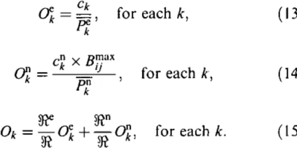
Ck0%
=
=,
for each k,Pk
cn x STrlax nIl _ k IJ f h k Uk - pn or eac, k ( 13) ( 14) III is an independent M1M
[c
queuing system. That is, the service time is exponentially distributed with mean I!Ilk,and the rth priority lots have interarrival times that are exponentially distributed with rate },~ at the kth work-station. According to the non-preemptive priority queue model (Hiller and Lieberman, 1990; Winston, 1991), the queue time for the engineering lots and normal lots can be formulated as shown in Table I.
The above discussions show the procedure to estimate the loading-factor queue time for normal and engineering lots. The batching-factor queue time for a normal lot will be estimated by modifying the BFFT algorithm so as to fit with the existence of engineering lots. The core concept of the BFFT algorithm and the block definition will be discussed in detail in the next section.
3.2.7. Estimating the average service ratefor each workstation
The average service rate at workstation k, Ilk> is equal to
the product of the weighted average output rate for processing engineering lots and normal lots at the kth workstation. The Ilk can be written as:
( 16)
3.2.8. Estimating the queue time in a steady-state for engineering lots and normal lots at each workstation
The queueing model is an appropriate method to estimate the queue time incurred by an average workload at a workstation. Because of numerous re-entries to critical machines and different time lengths for arrival and service in each re-entry loop, it is assumed that each workstation
TableI, Non-preemptive priority queueing model
3.3. The definition and basic concept of a block
A block is defined as those batch and serial-type process steps delimited by the two nearest batch-type worksta-tions according to the process sequence (Chung and Huang, 1999). Since a batch-type workstation is an im-portant source of interference in the material flow, sepa-rating the whole process into numerous blocks can help us to analyze and identify material flow characteristics.
Due to the wafer fabrication complexity, there are three additional special block types besides the general block types defined above, as shown in Fig. 5. The basic definitions and the range covered are described below.
General Block Type: BSB
Both start and end process steps of the general block type individually being processed on batch-type workstations
Parameters Engineering 101(r
=
e) Normal lot(r=
n)w~ and
wf
\V~q and
wZ
qAk
General type
e
aa
e
Batch-Serial-Botch (BSB)«
complete type)Block Dtrio Front-end
0/
process (SB:type W no upstream batch workstation)
Special type ~-~~e Batch to batch (BB;
(incompletetype) /10serial workstation)
a a
Back-end ofprocess (BS;no downstream batch workstation)
Fig. 5. The definition of a block.
(B) and the process steps between them correspond to serial-type workstations (S).
Special Block Type: BB. SB and BS
Each of the following block types is an incomplete gen-cral-block type.
• The BB type: batch workstation to batch worksta-tion. Both start and end process steps belong to butch-type process (B). There is no serial-type pro-cessin between.
• The SB type: serial workstation to batch work-station. The start process step of the block is a serial-type process (S), and the end process step is a batch-type process (B). The SB type only occurs at the beginning of the whole process and it is an ex-ception of the general block type case.
• The BS type: batch workstation to serial work-station. The start process step of the block is a batch-type process (B), and the end process step is serial-type process (S). The BS type only occurs at the end of the whole process plan and is also an exception of the general block type case.
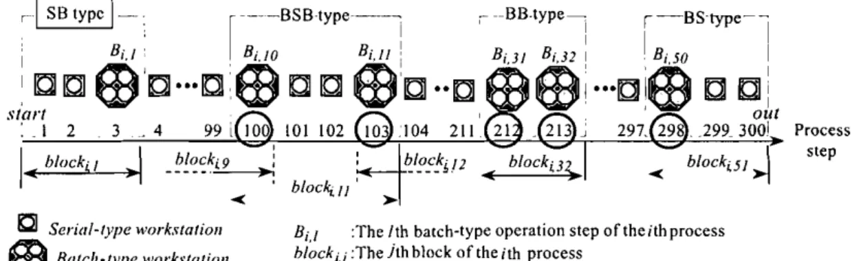
Figure 6 illustrates a wafer process in terms of blocks. It shows that the first block of the ith process is a SB type. It only appears once in the process and covers process steps I to 3. The II th block is classified as a BSB type, a general block type and covers process steps 100 to 103. The 32nd block is classified as a BB type and covers process step 212 to 213. The last block of the process is the 5\ st block, which is classified as a BS type; it appears only once in the process and covers process steps 298 to 300. Figure 6 shows that each complicated wafer fabri-cation process is made up of numerous blocks; each block can have different blocks and is categorized into one of BSB, BB, SB or BS types. To effectively estimate the cycle time for a lot flowing through the process, the material now characteristics for each block type must be clearly confirmed.
To confirm the material flow characteristics in a block, we must analyze the major factors that determine the lot
flow rate. Regardless how many process steps are included in each block, the lot flow rate in a block will be con-strained by the workstation with the lowest output rate. We define the workstation with the lowest output rate as the "critical workstation". Obviously, the critical work-station is the most important point at which to observe the material flow characteristics in the block and its output rate is the key value. Notice that the critical workstation may be a batch-type or a serial-type. After a lot completes the critical operation step, it will go through downstream process steps in the block at an output rate that is rela-tively faster than that in the critical workstation.
In addition to the critical workstation, the batch characteristics of the two batch workstations also affects the material flow. For each block, the material flow may be interrupted before the second batch workstation be-cause the minimum batch size condition has not been met. This characteristic of wafer lots waiting for batch formation has made the second batch workstation play the role of a material flow interrupter.
Furthermore, when multiple lots are released from the first batch machine of a block, a temporarily peak load may occur in the downstream workstation. This severely disturbs the smoothness of the material flow. Thus, the first batch workstation also plays the rather important role of material flow disturbance.
Combining the above discussions, the material flow for the block will be affected by: (i) the output rate and the batch size setting of the first and second batch worksta-tions; and (ii) the output rate of the workstation with the lowest output rate among all serial workstations in the block. These three important workstations are defined here as material flow observation points.
The product mix ratio and the throughput target of a planning period will affect the output rate of each workstation. The three observation points must be con-firmed whenever the throughput target or the product mix ratio is changed. Once the interactions among them are confirmed, we can effectively recognize the material flow in the entire block and then catch the cycle time characteristics.
BU :TheIth batch-type operation step oftheithprocess b10ckiJ:Thehh block of the ith process
r-BStype-~ I I I
n
I1J
j out 297. 298 .. 299. 3001 -e block,5!~
~ ~BBtype-s-, I -~-BSBtype ---~ h/ocki,9 ]----_.=---~I
C
Serial-type workstationm
Batch-type workstationFig. 6. Process nowin terms of blocks.
Cycle time estimation for wafer fab
BBCT methodology (Chung and Huang, 1999) applies the block concept and uses the output characteristics of the material flow observation points to estimate the batching-factor queue time (T~) and the theoretical pro-cess time(Tp ) .The BBCT methodology assumes that the lots in the wafer fab are all normal lots and the batch-factor queue time for each lot is estimated under the assumption that all the available capacity of each work-station can be used for producing normal lots. However, the available capacity for normal lots will decrease when an engineering lot is introduced into the fab. Therefore, it is necessary to revise the available capacity formulae for engineering lots and normal lots. The next section states how to revise the available capacity for normal lots.
3.4. Calculation of the hatching-factor queue time
An engineering lot does not have a batching-factor queue time; it only has a loading-factor queue time, which is estimated by using the non-preemptive priority queue model as stated before.
When estimating the Batching-Factor Flow Time (BFFT) for normal lots, the q values in each formula for block time calculation, developed by Chung and Huang (1999), is replaced by
cZ
in order to transform the cycle time estimation algorithms that do not consider engi-neering lots into algorithms that do consider engiengi-neering lots. The BBCT model with a consideration of engineer-ing lots is thus symbolized as BBCTe.4. Experimental design and results
In order to evaluate the performance accuracy of BBCTe on cycle time estimation, a wafer fab simulation model is constructed. The cycle time estimation by BBCTe is compared with a simulation result in order to understand the performance accuracy. The simulation model applies the actual production data obtained from a real wafer fab. These input data include three major factors, prod-ucts, equipment and processes, as described below:
113 I. Product related data: There are five products, Products A, B, C, D and E in the model with a product mix of 5: 7: 3: 4: I in sequence, (i.e. 25, 35, 15,20 and 5% respectively) and a weekly wafer re-lease quantity of 4000 wafers. Product E is assumed to be an engineering lot. The release policy is ap-plied with the fixed-WIP method. Each release quantity for Products A to 0 is 150 wafer pieces (or six lots) and each release quantity for Product E is 25 wafer pieces (or one lot).
2. Process related data: Products A to E corresponds to processes A to E, where the first two products are logic products and the others are memory products. The number of process steps is between 276 and 345. 3. Equipment related data: In the fab, 236 machines are separated into 83 different types of workstations, of which 37 are batch workstations. The maximum batch size for a batch workstation can be classified into six, four and two lots, each with 15, three and 19 machine types. Every workstation applies the FIFO dispatch rule, and every batch workstation applies the full-load batch rule, except for engi-neering lots.
The total simulation time is 240 days, of which the first 60 days is the system warm-up stage. To explain that both the BBCTO and BBCT have a satisfactory accurate performance for cycle time estimation in a system envi-ronment with existing and non-existing engineering lots, respectively, a simulation will be carried out to show the results under these two different conditions. In addition to the experimental design, the Appendix will show a simple example to describe how to calculate the lot cycle time.
4.1. Experiment I: no engineering lots
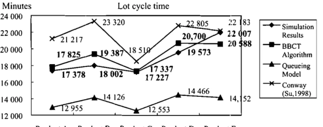
Figure 7shows a comparison of the average lot cycle time for each product type estimated by using simulation, BBCT methodology (including hand TB) , M / M /c
queueing model (Hiller and Lieberman, 1990; Winston,
Minutes Lot cycle time
24000 22 83 22000 2.2 07 20 88 20000 18000 16000 14000 14, 52 12000
ProductA ProductB ProductC ProductD ProductE
-+-Simulation Results ---BBCT Algorithm
-+-
Queueing Model ~Conway (Su,1998)Fig. 7. The lot cycle time for each product type (after Chung and Huang (1999».
35.7 --+--BBCT Algorithm - - - QueueingModel -+-Conway S 1998
-+.___-=-"...-..
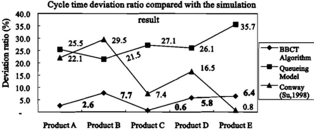
6.4 I'---'=:'::":"::L-I 0.8 Cycle time deviation ratio comparedwith the simulationresult 40.0
--~ 35.0'f
30.0g
25.0 ~ 20.0!
15.0 10.0 5.0ProductA Product B Product C Product D Product E
Fig. II. A comparison of the estimation accuracy among cycle time estimation methods (after Chung and Huang (1999)).
1991) and Su's estimation formula (Su, 1998). The ratios for deviation from simulation results are shown in Fig. 8. The absolute values for the minimum deviation ratio, the maximumdeviation ratio and the average deviation ratio can be read as (0.06, 7.7, 4.9%), (21.5, 35.7, 25.0%) and (0.8,29.5,20.3°;'.) by using the BBCT algorithm, general
M 1M
[c
queue model and Su's estimation formula re-spcctivcly. The above average deviation ratio is weighted based on the product mix ratio. Apparently, the cycle timc estimation performance resulting from the BBCT algorithm including the minimum deviation ratio, maxi-mumdeviation ratio and the average deviation ratio is a significant improvement over the other methods.4.2. Experiment 2: where product E isall engineering lot Here, Product E is in accordance with the dispatching principles for engineering lots. Figure 9 shows the changes in each product cycle time before and after
en-gineering lots arc placed into the system. As far as Product Eis concerned, the average lot cycle time drop-pcd from the original 22 007 minutes to 14 193 minutes, or by approximately 57.4% in cycle time length, after the lot attribute was changed to an engineering lot. On the other hand, thc average lot cycle time for Products A to D increased by 4.8% to 12.5%. As the above results show, thc engineering lot's eycle time will sharply
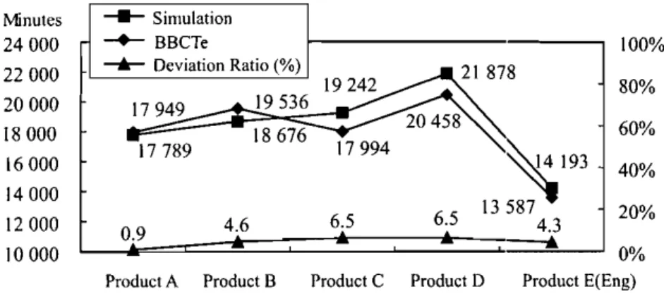
de-crease and the normal lot's cycle time will inde-crease after engineering lots are placed into the system. Figure 10 shows a comparison of the cycle time estimation using BBCT" and simulation results. Since the estimated cycle time for Product E is 13587 minutes and its simulation result is 14193 minutes, there is a 4.3% deviation ratio. Also, the deviation ratios between the estimated cycle time and simulation results for normal Products A to D is between 0.9 and 6.5%. Hence, BBCT" has a very good estimation performance when engineering lots exist in the system.
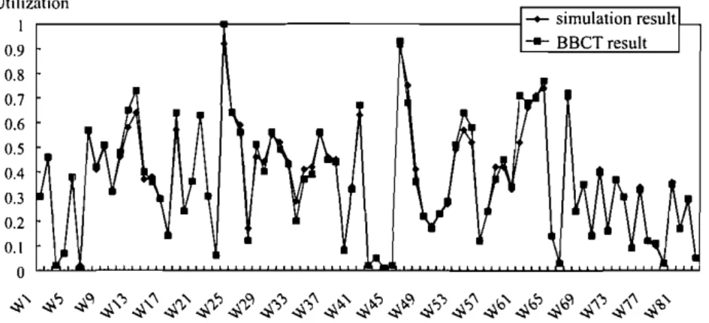
It is known that there is a direct connection between the length of the loading-factor queue time and the workstation utilization. In order to ensure that the loading-factor queue time estimation is reasonable, this experiment has further demonstrated the estimation ac-curacy of BBCT" in estimating each workstation's utili-zation rate. The results show that there are approximately 66.2,89.2 and 98.9% of the total number of workstations whose difference in machine utilization rate between the BBCT" estimated value and the simulation result is less than 0.01, 0.05 and O.I respectively. There is only one workstation, or approximately 1.2% of the total number of workstations, that has more than 0.1 as the difference between its BBCT estimate and its simulation result. The mean and standard deviation for the absolute differences in estimating machine utilization is 2 and 2.97%
respec-120% 0% -40% 40% 80%
-+-
No Eng lots-+-
With Eng lots-+-
Cycle time change ratio(%-80% Product A Product B Product C Product D Product E(Eng) 25000
20000 15000 10000 5000
Fig. 9. Thc average cycle time changes before and after an engineering lot is introduced.
Cycle time estimation for wafer Jab
115 ... Simulation-+-
BBCTe ... Deviation Ratio(%) 80% 60% 20% 40% 100% 0% Product E(Eng)~193
6 5. 135874.3--...
Product D 6.5 Product C 4.6 Product B 17949 17789 0.9 Product A Minutes 24000 22000 20000 18000 16000 14000 12000 10 000Fig.
to.
The cycle time deviation between the BBCT' and simulation results. tively. Therefore, BBCl" also has an outstandingper-formance in estimating the workstation utilization, and consequently the accuracy in estimating the loading-fac-tor queue time is effectively confirmed. The comparison between the estimated utilization by BBCl" and the re-spective simulation result is listed in Table 2and depicted in Fig. 11.
5. Conclusions and future research
When a wafer lot is processed in a wafer fab, not only the machine load factors but also the machine batch size attributes may affect queue time formation. Inthis paper,
the queue time formation for a wafer lot is divided into two categories: the loading-factor, resulting from the
machine load, and the hatching-factor, resulting from the
batch size setting for the batch machine. The queue time accrued from the loading-factor is estimated by applying the non-preemptive priorityM 1M
Ie
queue model (Hiller and Lieberman, 1990; Winston, 1991), while the queue time accrued from the batching-Iactor is estimated by applying the BFFT algorithm when engineering lots exist in the system. The cycle time estimation methodology developed in this paper is symbolized as BBC'fC. The distinctive feature of the of the BBCl" model is that all the calculations are in arithmetic form, and hence the computation time is really short.Table2. A comparison of the machine utilization rates
Work- Simulation BBCT' Work- Simulation BBCT' Work- Simulation BBCT' Work- Simulation BBCT'
station result station result station result station result
WI 0.30 0.30 W22 0.30 0.30 W43 0.05 0.05 W64 0.74 0.77 W2 0.45 0.46 W23 0.06 0.06 W44 0.01 0.01 W65 0.14 0.14 W3 0.02 0.02 W24 0.92 1.00 W45 0.02 0.02 W66 0.03 0.03 W4 0.07 0.07 W25 0.64 0.64 W46 0.91 0.93 W67 0.70 0.72 W5 0.37 0.38 W26 0.59 0.56 W47 0.75 0.68 W68 0.25 0.24 W6 0.02 0.01 W27 0.17 0.12 W48 0.41 0.36 W69 0.35 0.35 W7 0.56 0.57 W28 0.46 0.51 W49 0.22 0.22 W70 0.15 0.14 W8 0.41 0.42 W29 0.44 0.40 W50 0.18 0.17 W7I 0.41 0.40 W9 0.50 0.51 W30 0.55 0.56 W51 0.23 0.23 W72 0.17 0.16 WIO 0.32 0.32 W31 0.52 0.49 W52 0.27 0.28 W73 0.37 0.37 WII 0.46 0.48 W32 0.44 0.43 W53 0.49 0.51 W74 0.30 0.30 WI2 0.58 0.65 W33 0.28 0.20 W54 0.57 0.64 W75 0.10 0.09 WI3 0.64 0.73 W34 0.41 0.37 W55 0.52 0.58 W76 0.34 0.33 WI4 0.37 0.40 W35 0.42 0.39 W56 0.12 0.12 W77 0.12 0.12 WI5 0.38 0.36 W36 0.56 0.56 W57 0.24 0.24 W78 0.10 0.11 WI6 0.29 0.29 W37 0.46 0.45 W58 0.42 0.37 W79 0.03 0.03 WI7 0.15 0.14 W38 0.45 0.44 W59 0.42 0.45 W80 0.36 0.35 WI8 0.57 0.64 W39 0.09 0.08 W60 0.33 0.34 W81 0.17 0.17 WI9 0.24 0.24 W40 0.34 0.33 W61 0.52 0.71 W82 0.28 0.29 W20 0.36 0.36 W41 0.63 0.67 W62 0.66 0.68 W83 0.05 0.05 W21 0.63 0.63 W42 0.02 0.02 W63 0.71 0.70
Utilization .... BBCT result . - - - -...- - - l - + - simulation result I 0.9 0.8 0.7 0.6 0.5 0.4 0.3 0.2 0.1 o
~~~~~~~~~~~~~~fi~~~~~~
Fig. IJ. A comparison between the utilization estimate for each workstation by the BBCT' algorithm and the simulation results.
A simulation model was built based on the production data from a real wafer fab in Taiwan. In the "no engi-neering lots" scenario, the lot eyele time estimated by BBCT was very close to the simulation results. The av-erage deviation ratio was merely 4.9%, which shows that the BBCT methodology clearly performs better than the other methods in cycle time estimation. Under the "en-gineering lots present" scenario, the BBCTc model
showed a satisfactory performance estimation with the average deviation ratio to approximately 4.6%. The re-luted experiment also shows that BBCTc can effectively estimate the workstation utilization.
In this paper, the BBCTc is used to estimate the cycle time of two-priority class lots, that is, engineering lots and normal lots. In our future research, the
multiple-priority class will be considered into the model.
Acknowledgements
This paper was supported in part by the National Science Council, Taiwan, ROC, under Contract No
NSC88-2213-E009-027.
References
Atherton. L.F. andAtherton, R.W. (1995) W(ifer Fabrication: Factory
Perfonnnnce and Analysis, Kluwer, Massachusetts.
Chung. S.H. and Huang, H.W. (1999) The block-based cycle time es-tinuuion algorithm for wafer fabrication factories. International
Journal (If Industrial Engineering, 6(4), 307-316.
Conway, R., Maxwcll, W. and Miller, L.W. (1967) Theory (If Sched-uling, Addison-Wesley, Massachusetts.
Cunningham. J.A. (1990) The usc and evaluation of yield model in integrated circuit manufacturing. IEEE Transactions on Semi-conductor Manufacturing, 3(2), 60-72.
Enns S.T. (1995) A dynamic forecasting model for job shop flowing prediction and tardiness control. International Journal of Pro-duction Research. 33(5), 1295-1312.
Etheshami. B., Petrakian, R.G. and Shabe, P.M. (1992) Trade-offs in cycle time management: hot lots. IEEE Transactions on
Semi-conductor Manufacturing, 5(2), 10I-I05.
Fowler, J.W., Philips, D.T. and Hogg, G.L. (1992) Realtime control of multiproduct bulk-service semiconductor manufacturing process-es. IEEE Transactions on Semiconductor Manufacturing, 5(2),
158-163.
Fronckowiak, D., Peilert, A. and Nishinohara, K. (1996) Using dis-crete event simulation to analyze the impact of job priorities on cycle time in semiconductor manufacturing, in Proceedings of the 1996 IEEE/SEMI Advanced Semiconductor Munufacturing Conference, New York, pp. 151-I55.
Glassey, CR. and Resende, M.G.C (1988) Closed-loop job release control for VLSI circuit manufacturing. IEEE Transactions on Semiconductor Manufacturing, 1(1), 36-46.
Glassey, CR. and Weng, W.W. (1991) Dynamic hatching heuristics for simultaneous processing. IEEE Transactions 011 Semiconductor
Manufacturing, 4(2), 77-82.
Hiller, F.S. and Lieberman, G.J. (1990) Introduction to Operations Research, 51h edn. McGraw-Hili, New York.
Kaplan, A.C and Unal, A.T. (1993) A probabilistic cost-based due date assignment model for job shops. International Journal
01
Production Research, 31(12), 2817-2834.Kim, Y.D., Kim, J.-U., Lim, S.-K. and Jun. H.-B. (1998) Due-date based scheduling and control policies in a multiproduct semi-conductor wafer fabrication facility. IEEE Transactions on
Semiconductor Manufacturing, II (I), 155-164.
Martin, D.P. (1998) How the law of unanticipated consequences can nullify the theory of constraint: the case for balanced capacity in a semiconductor manufacturing line, Semiconductor Fabtech, 7th
edn, ICG Publishing Ltd, pp. 29-34.
Matsuyama, A. and Atherton, R.W. (1990) Experience in simulation wafer fabs in the USA and Japan, in Proceedings of tile 1990 International Semiconductor Manufacturing Science Symposium,
Burlingame, USA, pp. 113-118.
Miller, D.J. (1989) Implementing the results of a simulation in a semiconductor line, in Proceedings
01
the 1989 Winter Simulation Conference, New York, pp. 922-929.Narahari, Y. and Khan, L.M. (1997) Modeling the effect of hot lots in semiconductor manufacturing systems. IEEE Transactions on Semiconductor Manufacturing, 10(1), 185-188.
Raddon, A. and Grigsby, B. (1997) Throughput time forecasting model, in Proceedings of tile 1997 IEEE/SEMI Advanced Semi-conductor Manufacturing Conference, pp. 430-433.
Su, Y.C (1988) The construction of production planning and sched-uling system for an IC foundry in ramp-up., Masters thesis,
Cycle time estimation for wafer fab
dustrial Engineering and Management Department, National Chiao Tung University, Hsin-Chu, Taiwan.
Vig, M.M. and Dooley, KJ. (1991) Dynamic rules for due-date as-signment. lnternational Journal of Production Research, 29(7),
1361-1377.
Wein, L.M. (1988) Scheduling semiconductor wafer fabrication. 1£££ TransactionsonSemiconductor Manufacturing, 1(3), 115-130. Winston, W.L. (1991)Operations Research: Applications and
Algo-rithms, PWS-Kent, Boston, MA.
Wood, S.c. (1997) Cost and cycle time performance of fabs based on intergrated single-wafer processing.1£££ Transactions on
Semi-conductorManufacturing, 10(1),98-111.
Appendix
A simple model
A simple model is built in order to explain that of BBCTe, procedure. Assume that a system has only two
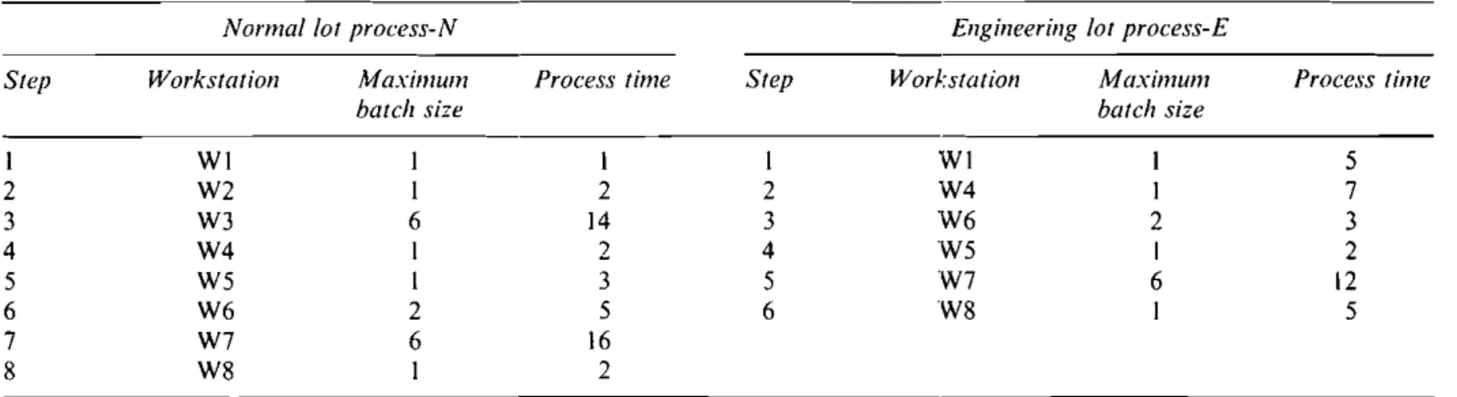
prod uct types, normal lots and engineering lots, corre-sponding to process Nand E. The product mix of Nand E is 30:I. The process related information including process steps, workstation, and process time is shown in Table AI.
Table A2 shows the workstation related information. There are eight workstations in this system. Each
work-117 station has a only one machine that has a 100 time unit capacity (I time unit = 14.4 minutes) per day. Machines never break down or need maintenance. Based on the above information,
ci
andcr
can be estimated by using Equations (4)-(10).According to the definition of the block, the normal lot process is segmented into four blocks that are classified as SB, BSB, BB and BS in sequence. Based on the block style, the batching-factor flow time of each block can be effectively estimated by using the BFFT algorithm and replacing the Ck defined in Chung and Huang (1999)
by
cr.
Moreover, the batching-factor flow time of the entire process cart also be estimated by using the formula for the multiple-block cycle time developed in Chung and Huang (1999).The result is shown in Table A3. Note that in Table A3 the flow time of the normal lot was calculated as:
Flow time of normal lot
=
27+
42+
52+
46 - 14x
r6~
cl- 5X
r2X~.97l
- 16x
r
6x~.88l
= 101.TableAI. Process-related information
Normal lot process-N Engineering lot process-E
Step Workstation Maximum Process time Step Workstation Maximum Process Iime
batch size balch size
I WI I I I WI I 5 2 W2 I 2 2 W4 1 7 3 W3 6 14 3 W6 2 3 4 W4 I 2 4 W5 I 2 5 W5 I 3 5 W7 6 12 6 W6 2 5 6 W8 I 5 7 W7 6 16 8 W8 I 2
TableA2. Workstation-related information Workstation WI W2 W3 W4 W5 W6 W7 W8 Workstation type
s
S B S S B B S Maximum batch size I I 6 I I 2 6 I Available EQ num (Ck) Occupied by engineering lots (c,) 0.05 0.00 0.00 0.07 0.02 0.03 0.12 0.05Reserved for normal lois (c'k) 0.95 1.00 1.00 0.93 0.98 0.97 0.88 0.95
Lor rype
Normal lot Engincering lot
Barch factor Loading [actor Lor cycle rime Simulation Deviation ratio (%)
flow lime queueing time estimated by BBCT' cycle rime ((C)-(D))/(D)
(A) ( B) (C)=( A)+(B) (D)
101.0 105.1 206.1 192.9 6.8
34.0 14.5 48.5 48.0 1.0
Thc calculation is based on Equation (28)in Chung and Huang (1999). Similarly, the batching-factor flow time for thc engineering lot can also be estimated according to thc procedure mentioned above. The result is shown in Table A4. Finally, the loading-factor queue time is esti-mated by using the non-preemptive priority queue model mentioned in Section 3.2.
Notc that thc flow time of the engineering lot was calculated as:
Flow time of engineering lot = 15
+
17+
17 - 3xr2~ll-12
x
r
6XT
Il
=
34. Thc calculation is based on Equation (28)in Chung and Huang (1990).To evaluate the accuracy performance of the cycle timc estimation, a simulation model is constructed. Table A5 shows a comparison between the lot cycle time estimated by the BBCTc methodology and its respective
simulation result. The average lot cycle time deviation ratios of the normal and engineering lots are only 6.8 and 1.0%, respectively. This demonstrates that the BBCT" algorithm can produce a satisfactory cycle time estimation.
Biographies
Dr. S.H. Chung is a Professor in the Department of Industrial Engi-neering and Management, National Chiao-Tung University, Taiwan, ROC. She received a Ph.D. degree in Industrial Engineering from Texas A&M University, College Station, TX, USA. Her research in-terests include production planning, scheduling, system simulation, and production planning of IC manufacturing. She has published and presented research papers in the areas of production planning, sched-uling, cost analysis and IC manufacturing management.
Hung-Wen Huang is a Ph.D. candidate at the Department of Indus-trial Engineering and Management, National Chiao-Tung University, Taiwan, ROC. He received his M.S. degree in Industrial Engineering and Management from National Chiao-Tung University. He is also a Manager in the Department of Operation Analysis, Winbond Elec-tronic Corp., Taiwan, ROC. His research interests include operation and performance analysis in the semiconductor industry.