Applying Particle Swarm Optimization to Parameter Estimation of the Nonlinear Muskingum Model

Applying Particle Swarm Optimization to Parameter

Estimation of the Nonlinear Muskingum Model

Hone-Jay Chu

1

and Liang-Cheng Chang

2

Abstract: The Muskingum model is the most widely used method for flood routing in hydrologic engineering. However, the application of the model still suffers from a lack of an efficient method for parameter estimation. Particle swarm optimization共PSO兲 is applied to the parameter estimation for the nonlinear Muskingum model. PSO does not need any initial guess of each parameter and thus avoids the subjective estimation usually found in traditional estimation methods and reduces the likelihood of finding a local optimum of the parameter values. Simulation results indicate that the proposed scheme can improve the accuracy of the Muskingum model for flood routing. A case study is presented to demonstrate that the proposed scheme is an alternative way to estimate the parameters of the Muskingum model.

DOI: 10.1061/共ASCE兲HE.1943-5584.0000070

CE Database subject headings: Flood routing; Optimization; Parameters; Estimation; Hydrologic models; Particles.

Introduction

Among the many models used for flood routing, the Muskingum method is the most widely used owing to its simplicity. The Muskingum flood routing model was developed by the U.S. Army Corps of Engineers for the Muskingum Conservancy District Flood-Control Project over six decades ago. The following conti-nuity and nonlinear storage equations are commonly used in the Muskingum model共Gill 1978; Tung 1985; Yoon and Padmanab-han 1993; MoPadmanab-han 1997; Kim et al. 2001; Geem 2006; Al-Humoud and Esen 2006兲

dSt

dt = It− Ot 共1兲

St= K关XIt+共1 − X兲Ot兴m 共2兲 where S_t, I_t, and O_tdenote the instantaneous amounts of storage, inflow, and outflow, respectively, at time t; K = storage-time con-stant for the river reach, which has a value reasonably close to the flow travel time through the river reach; X = a weighting factor usually varying between 0 and 0.5 for reservoir storage, and be-tween 0 and 0.3 for stream channels; and m = an exponent for considering the effects of nonlinearity. However, the calibration for finding the optimal value of the three parameters K, X, and m can be complicated.

Over the last two decades, many optimization techniques, in-cluding Broyden-Fletcher-Goldfarb-Shanno method, genetic

algo-rithm共GA兲, and harmony search 共HS兲, etc., have been applied to identify the three parameters 共Gill 1978; Tung 1985; Yoon and Padmanabhan 1993; Mohan 1997; Kim et al. 2001; Geem 2006兲. Gill共1978兲 used a least-squares method 共LSM兲 to find the values of the three parameters in the nonlinear Muskingum model. Tung 共1985兲 proposed parameter estimation using the Hook-Jeeves 共HJ兲 pattern search in conjunction with linear regression 共LR兲, the conjugate gradient 共CG兲, and Davidon-Fletcher-Powell 共DFP兲 techniques. The performance of the methods was compared with Gill’s procedure and 共HJ+CG兲 and 共HJ+DFP兲 were found to yield better solutions. Yoon and Padmanabhan 共1993兲 discussed several methods for estimating the parameters. The linear model may be inappropriate when the nonlinear relationship between the storage and discharge exists in most actual river systems. The suggested method for the nonlinear routing model is an iterative procedure and involves the nonlinear least-squares regression 共NONLR兲. Mohan 共1997兲 pointed out all of the foregoing meth-ods do not guarantee the global optimal, and they may be trapped at a local optimum. He used GA to estimate the parameters in the model. The results showed that the estimation by GA was better than by the previous methods and did not require the initial guess to be close to the optimum. Kim et al.共2001兲 applied the HS to the same problem. Their results showed HS estimation was better than GA and also did not require that the initial guess were close to the optimum.

In this study, the parameter estimation for the nonlinear Musk-ingum model is performed using the particle swarm optimization 共PSO兲 technique. The results are then compared to those obtained using the previous described techniques.

Routing Procedure of the Nonlinear Muskingum Model

By rearranging Eq.共2兲, the rate of the outflow can be expressed as Ot=

冉

1 1 − X

冊冉

St K

冊

1/m −

冉

X 1 − X

冊

It 共3兲

Combining Eq. 共3兲 and the continuity Eq. 共1兲, the state equation can be obtained as

1

Postdoctoral Fellow, Dept. of Bioenvironmental Systems Engineer-ing, National Taiwan Univ., Taipei, Taiwan 10617, Republic of China 共corresponding author兲. E-mail: honjaychu@gmail.com

2

Professor, Dept. of Civil Engineering, National Chiao Tung Univ., 1001 Ta Hsueh Road, Hsinchu, Taiwan 30050, Republic of China.

Note. This manuscript was submitted on March 13, 2008; approved on January 13, 2009; published online on February 18, 2009. Discussion period open until February 1, 2010; separate discussions must be submit-ted for individual papers. This technical note is part of the Journal of

Hydrologic Engineering, Vol. 14, No. 9, September 1, 2009. ©ASCE,

ISSN 1084-0699/2009/9-1024–1027/$25.00.

1024 / JOURNAL OF HYDROLOGIC ENGINEERING © ASCE / SEPTEMBER 2009

J. Hydrol. Eng. 2009.14:1024-1027.

⌬St ⌬t = −

冉

1 1 − X

冊冉

St K

冊

1/m +

冉

1 1 − X

冊

It 共4兲 St+1= St+⌬St 共5兲 Ot+1=

冉

1 1 − X

冊冉

St+1 K

冊

1/m −

冉

X 1 − X

冊

I ¯ t+1, where I¯t+1=共It+1+ It兲/2 共6兲 The routing procedure involves the following steps共Geem 2006兲: Step 1. Assume values for the three parameters, K, X, and m.

Step 2. Calculate storage共St兲 using Eq. 共2兲, where initial

out-flow is same as initial inout-flow.

Step 3. Calculate the time rate of change of storage volume using Eq.共4兲.

Step 4. Estimate the next accumulated storage using Eq.共5兲.

Step 5. Calculate the next outflow using Eq. 共6兲. I¯t+1 is

ex-pressed as average inflow共It+1+ It兲/2. Itreplaces共It+1+ It兲/2 when the ratio of storage t and t + 1 is over 2.

Step 6. Repeat Steps 2–5.

PSO

PSO is a stochastic optimization technique developed by Kennedy and Eberhart共1995兲, inspired by social behavior of bird flocking or fish schooling共Clerc and Kennedy 2002兲. PSO pro-vides a population-based search procedure in which individuals called particles change their position with time. In the past several years, PSO has been successfully applied including hydrological modeling. For example, Chau共2004兲 used a PSO model adopted to train perceptrons. The perceptron is a type of artificial neural network which the inputs are fed directly to the outputs via the weighted connections. The optimal weightings are determined by PSO in training process. The approach is demonstrated to be fea-sible and effective by predicting real-time water levels in the Shing Mun River of Hong Kong with different lead times on the basis of the upstream gauging stations or stage/time history at the specific station. Chau共2005兲 also presented the application of a split-step PSO model for training perceptrons to forecast real-time algal bloom dynamics in Tolo Harbour of Hong Kong. In this study, parameter estimation for the nonlinear Muskingum model using the PSO is developed.

In a PSO system, particles fly around in a multidimensional search space. During flight, each particle adjusts its position ac-cording to its own experience, and acac-cording to the experience of a neighboring particle, making use of the best position encoun-tered by itself and its neighbor. PSO shares many similarities with evolutionary computation techniques such as GA 共Clerc and Kennedy 2002; Boeringer and Werner 2004; Robinson and Rahmat-Samii 2004兲. The system is initialized with a population of random solutions and searches for optima by updating genera-tions. However, unlike GA, PSO has no evolution operators such as crossover and mutation. The PSO algorithm can be expressed as follows: At kth iteration, a current ith particle position in the multidimensional search space which represents 共Yik_{兲. A current}

velocity 共V_ik兲 controls its fly speed and direction. The velocity each particle updates along each dimension toward local and glo-bal best positions in Eq. 共7兲, and the position update in Eq. 共8兲 that are given by

V_ik+1= V_ik+ c1r1共Pik− Yi k_{兲 + c}

2r2共Pgk− Yi

k_{兲 共7兲}

Y_ik+1= Y_ik+ V_ik+1 共8兲

where Pi= best previous position of particle共also known as pbest兲; Pg= global best position among all the particles 共also known as gbest兲; c1 and c2= constants known as acceleration coefficients which control how far a particle will move in a single iteration; and r1and r2= elements from two uniform random numbers in the range共0, 1兲.

Eqs.共9兲 and 共10兲 update the local bests 共Pi兲 and the global best 共Pg兲 Pi=

再

Pi:f共Yi兲 ⱖ f共Pi兲 Yi:f共Yi兲 ⬍ f共Pi兲

冎

共9兲 Pg= min关f共Pi兲兴, i = 1,2, ... ,M 共10兲 where f = the objective function and M = the total number of par-ticles.

Application

Outflow hydrographs along with routed flows can be obtained using the proposed nonlinear Muskingum model. To investigate the performance of PSO, a typical problem is used as an example. PSO for the estimating of the parameters in the nonlinear Musk-ingum model was applied to an example which was first proposed by Wilson共1974兲. The ranges of three parameters in the nonlinear Muskingum model are K = 0.01– 0.20, X = 0.2– 0.3, and m = 1.5– 2.5. The objective function of PSO is to minimize the sum of the squared deviations共SSQs兲 between the computed and ob-served outflows

Minimize SSQ =

兺

t=1 n

共Ot− Oˆt兲2 共11兲 where Oˆt denotes the computed outflow at time t. In this PSO algorithm, a population of 100 individuals is used. The maximum number of iterations in the program is 100. The values of the acceleration constants共c₁and c₂兲 are both set to 1.0.

Fig. 1 shows a comparison of the performances of the different parameter estimation procedures. Columns 1–3 of Table 1 are the actual data 共Wilson 1974兲; columns 4–9 show the routed flow data obtained by using the Muskingum model. Column 4 uses the LSM共Gill 1978兲; Column 5 uses the HJ+DFP 共Tung 1985兲; Col-umn 6 uses NONLR 共Yoon and Padmanabhan 1993兲; Column 7 uses GA共Mohan 1997兲; Column 8 uses HS 共Kim et al. 2001兲; Column 9 uses PSO programs to estimate the parameters which are then used to determine the routed flows.

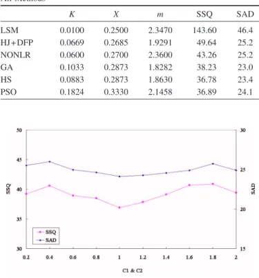
Finally, the new method 共PSO兲 and the five conventional methods are compared using the SSQ and sum of absolute devia-tions共SADs兲 between the computed and observed outflows pre-sented in Table 2. The results show that the SSQ is attained using PSO. It has been demonstrated that PSO gets better results than other methods except HS. Fig. 2 shows the sensitivity of SSQ and SAD to the PSO parameters 共c1and c2兲.These parameters range from 0.2 to 2. The finding implies clearly that the value of SSQ is JOURNAL OF HYDROLOGIC ENGINEERING © ASCE / SEPTEMBER 2009 / 1025

J. Hydrol. Eng. 2009.14:1024-1027.

the minimum for the example studied when c1= 1 and c2= 1. Thus, the PSO yielded good SSQ and SAD over a wide range of c1and c2values.

Conclusions

The newly developed heuristic algorithm, PSO, is applied to the parameter estimation problem of the nonlinear Muskingum model. While possessing similar capabilities to the GA, the par-ticle swarm model is much simpler to implement. The proposed

approach is compared with the other optimization methods for an example case from the literature. PSO has the advantage that it does not require assumption of the initial values of the model parameters. The results demonstrate that PSO can achieve a high degree of accuracy to estimate the three parameters and this re-sults in accurate predictions of outflow. Consequently, the model also shows robustness in forecasting outflow. With the PSO method, no derivative is required, and the semibiological evolu-tion will approach the nearly global optimum soluevolu-tion. PSO ap-pears to offer good applicability in the hydrology field and further applications should be explored.

Acknowledgments

The writers thank the editors, anonymous reviewers, and helpers.

References

Al-Humoud, J. M., and Esen, I. I.共2006兲. “Approximate methods for the estimation of muskingum flood routing parameters.” Water Resour. Manage., 20, 979–990.

Boeringer, D. W., and Werner, D. H.共2004兲. “Particle swarm optimiza-tion versus genetic algorithms for phased array synthesis.” IEEE Trans. Antennas Propag., 52共3兲, 771–779.

Chau, K.共2004兲. “River stage forecasting with particle swarm optimiza-tion.” Lect. Notes Comput. Sci., 3029, 1166–1173.

Chau, K. W.共2005兲. “A split-step PSO algorithm in prediction of water quality pollution.” Advances in Neural Networks—ISNN 2005, PT 3, Proc., 3498, 1034–1039.

Clerc, M., and Kennedy, J.共2002兲. “The particle swarm—Explosion, sta-bility, and convergence in a multidimensional complex space.” IEEE Trans. Evol. Comput., 6共1兲, 58–73.

Geem, Z. W.共2006兲. “Parameter estimation for the nonlinear Muskingum

Table 1. Inflow and Outflow Hydrographs for the Example and the

Results of Various Parameter Estimation Methods

Time 共h兲 Inflow共cms.兲 Observed outflow 共cms.兲 Computed outflow 共cms.兲 LSM HJ+ DFP NONLR GA HS PSO 0 22 22 22.0 22.0 22.0 22.0 22.0 22.0 6 23 21 22.0 22.0 22.6 22.0 22.0 22.0 12 35 21 22.8 22.4 23.0 22.4 22.4 22.6 18 71 26 29.6 26.7 24.2 26.3 26.6 28.1 24 103 34 39.1 34.8 33.2 34.2 34.4 32.2 30 111 44 47.6 44.7 47.1 44.2 44.1 45.0 36 109 55 58.0 56.9 56.8 56.9 56.8 57.0 42 100 66 67.1 67.7 66.2 68.2 68.1 67.5 48 86 75 74.8 76.3 75.0 77.1 77.1 75.9 54 71 82 80.4 82.2 80.7 83.2 83.3 81.2 60 59 85 83.2 84.7 83.5 85.7 85.9 85.6 66 47 84 82.8 83.5 84.3 84.2 84.5 84.2 72 39 80 80.1 79.8 79.9 80.2 80.6 79.6 78 32 73 74.5 73.3 74.3 73.3 73.7 73.3 84 28 64 67.2 65.5 65.3 65.0 65.4 65.0 90 24 54 58.1 56.5 55.9 55.8 56.0 56.2 96 22 44 48.1 47.5 45.1 46.7 46.7 46.5 102 21 36 37.6 38.7 35.4 38.0 37.8 37.3 108 20 30 28.2 31.4 28.7 30.9 30.9 29.7 114 19 25 21.9 25.9 24.3 25.7 25.3 24.3 120 19 22 19.1 22.1 20.9 22.1 21.8 20.6 126 18 19 19.0 20.2 20.4 20.2 20.0 19.6

Table 2. Estimated Parameters and Fit Quality Indicators Obtained by

All Methods K X m SSQ SAD LSM 0.0100 0.2500 2.3470 143.60 46.4 HJ+ DFP 0.0669 0.2685 1.9291 49.64 25.2 NONLR 0.0600 0.2700 2.3600 43.26 25.2 GA 0.1033 0.2873 1.8282 38.23 23.0 HS 0.0883 0.2873 1.8630 36.78 23.4 PSO 0.1824 0.3330 2.1458 36.89 24.1

Fig. 1. Inflow and outflow hydrographs for the example problem

computed with parameters obtained from selected estimation meth-ods

Fig. 2. Sensitivity of SSQ and SAD to selected values of c1and c2

1026 / JOURNAL OF HYDROLOGIC ENGINEERING © ASCE / SEPTEMBER 2009

J. Hydrol. Eng. 2009.14:1024-1027.

model using the BFGS technique.” J. Irrig. Drain. Eng., 132共5兲, 474– 478.

Gill, M. A.共1978兲. “Flood routing by Muskingum method.” J. Hydrol., 36共3–4兲, 353–363.

Kennedy, J., and Eberthart, R. C.共1995兲. “Particle swarm optimization.” Proc., IEEE Int. Conf. on Neural Networks, Piscataway, 1942–1948 Kim, J. H., Geem, Z. W., and Kim, E. S.共2001兲. “Parameter estimation of

the nonlinear Muskingum model using harmony search.” J. Am. Water Resour. Assoc., 37共5兲, 1131–1138.

Mohan, S.共1997兲. “Parameter estimation of nonlinear Muskingum mod-els using genetic algorithm.” J. Hydraul. Eng., 123共2兲, 137–142.

Robinson, J., and Rahmat-Samii, Y.共2004兲. “Particle swarm optimization in electromagnetics.” IEEE Trans. Antennas Propag., 52共2兲, 397– 407.

Tung, Y. K. 共1985兲. “River flood routing by nonlinear Muskingum

method.” J. Hydraul. Eng., 111共12兲, 1447–1460.

Wilson, E. M. 共1974兲. Engineering hydrology, MacMillan, Hampshire, U.K.

Yoon, J. W., and Padmanabhan, G.共1993兲. “Parameter-estimation of lin-ear and nonlinlin-ear Muskingum models.” J. Water Resour. Plann. Man-age., 119共5兲, 600–610.

JOURNAL OF HYDROLOGIC ENGINEERING © ASCE / SEPTEMBER 2009 / 1027

J. Hydrol. Eng. 2009.14:1024-1027.