線性矩陣不等式的強健適應滑差控制應用於T-S模糊系統

(1)

國立交通大學

電控工程研究所

博士論文

線性矩陣不等式的強健適應滑差控制應用

於 T-S 模糊系統

Linear Matrix Inequality Based Adaptive Sliding

Control for Takagi-Sugeno Fuzzy Systems

研究生：劉松傑

指導教授：林昇甫博士

(2)

線性矩陣不等式的強健適應滑差控制應用於 T-S 模糊系統

Linear Matrix Inequality Based Adaptive Sliding Control for

Takagi-Sugeno Fuzzy Systems

研究生：劉松傑

Student: Sung-Chieh Liu

指導教授：林昇甫博士

Advisor: Dr. Sheng-Fuu Lin

國立交通大學

電控工程研究所

博士論文

A Dissertation

Submitted to Institute of Electrical Control Engineering College of Electrical Engineering

National Chiao Tung University in Partial Fulfillment of the Requirements

for the Degree of Doctor of Philosophy

in

Electrical Control Engineering November 2012

Hsinchu, Taiwan, R.O.C 中華民國一Ο一年壹拾壹月

(3)

線性矩陣不等式的強健適應滑差控制應用

於 T-S 模糊系統

學生：劉松傑指導教授：林昇甫博士

國立交通大學電控工程研究所

摘要

物理系統自然形成非線性，因此，所有的控制系統都是具有某些程度的非線性。過去超過二十年時間，模糊技術已經廣泛地成功被利用在非線性系統模型建立與控制器設計。近十年來，T-S 模糊模型在處理複雜的非線性系統是一個廣為流傳且使用方便的工具。同樣地，對於非線性系統的模糊迴授控制設計問題已經廣泛地被研究藉由使用 T-S 模型，其中用簡單的局部線性模型被組合去描述非線性系統的全域行為。實際上，不可避免的不確定性也許會以一種非常複雜的方式進入到一個非線性系統模型。此不確定性也許包含模型誤差、參數變化、外部干擾和模糊近似誤差。在如此的一個情況下，模糊迴授控制設計方法也許不再運作良好。在本論文中，我們首先提出強健適應滑差控制（包含滑差控制和適應控制）應用於具有範數界限外部干擾的 T-S 模糊模式，同時放寬每一個正規的局部系統模式擁有相同輸入通道的限制假設，這個限制假設是傳統可變結構模糊控制設計方法所需要的。然後，提出具有非相配參數變動和外部擾動的 T-S 模糊模式之強健適應滑差控制。此外，針對具有非相配參數變動和外部擾動的 T-S 模糊時間延遲模式，其強健適應滑差控制亦被提出。最後，利用一些例子來驗證本論文所提出方法的有效性和可行性。關鍵字：T-S 模糊模式，範數界限變動，參數變動，外部擾動，滑差控制，適應控制。

(4)

ii

Linear Matrix Inequality Based Adaptive Sliding

Control for Takagi-Sugeno Fuzzy Systems

Student: Sung-Chieh Liu Advisor: Dr. Sheng-Fuu Lin

Institute of Electrical Control Engineering

National Chiao Tung University

ABSTRACT

Physical systems are inherently nonlinear. Thus, all control systems are nonlinear to a certain extent. Over the past two decades, fuzzy techniques have been widely and successfully exploited in nonlinear system modeling and control. In last ten years, the Takagi-Sugeno (T-S) fuzzy model is a popular and convenient tool for handling complex nonlinear systems. Correspondingly, the fuzzy feedback control design problem for a nonlinear system has been studied extensively by using the T-S model where simple local linear models are combined to describe the global behavior of the nonlinear system. In practice, the inevitable uncertainties may enter a nonlinear system model in a very complicated way. The uncertainty may include modeling errors, parameter variations, external disturbances, and fuzzy approximation errors. In such a situation, the fuzzy feedback control design methods may not work well anymore.

In this dissertation, firstly, we propose two kinds of LMI-based robust adaptive sliding control, including a robust sliding control method and a robust adaptive control method, for uncertain Takagi-Sugeno fuzzy models with norm-bounded uncertainties, and meantime relax the restrictive assumption that each nominal local system model shares the same input channel, which is required in the traditional VSS-based fuzzy control design methods. Then, two kinds of LMI-based robust adaptive sliding control are developed for uncertain T-S fuzzy models which include mismatched parameter uncertainties and external disturbances. Moreover, two kinds of LMI-based robust adaptive sliding control are proposed for the uncertain T-S fuzzy time-delay model which includes mismatched parameter uncertainties in the state matrix and norm-bounded external disturbances. Finally, some examples are used to illustrate the effectiveness and usefulness of the proposed methods in this dissertation.

Keywords: T-S fuzzy models, norm-bounded uncertainties, parameter uncertainties,

(5)

誌謝

這一路走來，終於等到榮耀的這一刻，感覺收獲良多，辛苦耕耘，含淚收割的果食真是甜美。回首這六年來的酸甜苦辣，有太多我需要感謝的人! 尤其是我的論文指導教授林昇甫老師。在此我要由衷地向您和師母表示十二萬分的謝意和敬意。由於您的鼎力相助、指導研究，並給予不斷的鼓勵，才能在遭受困挫時，使我越挫越勇而能更為精進。博士論文的完整性需要口試委員的指導，感謝我的口試委員—潘晴財教授、練光祐教授、張志永教授、董蘭榮教授和林錫寬教授，感謝您們在百忙中撥冗為我口試，因為有了您們的指導，學生的博士論文才能更臻完備。感謝電控系所和交大其它系所與單位，直接或間接指導、幫助過我的師長、先生和小姐們。同時，也要感謝實驗室內歷屆學長和學弟妹的協助和家人的支持。最後，恭謹地向所有關心、支持及協助我的人，表達我最誠摯的謝意。

(6)

ii

List of Figures

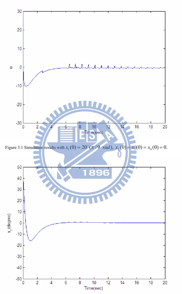
Figure 3.1 Simulation results withx₁(0)=20o(π/9 rad), x₂(0)=x₃(0)=x₄(0)=0.30

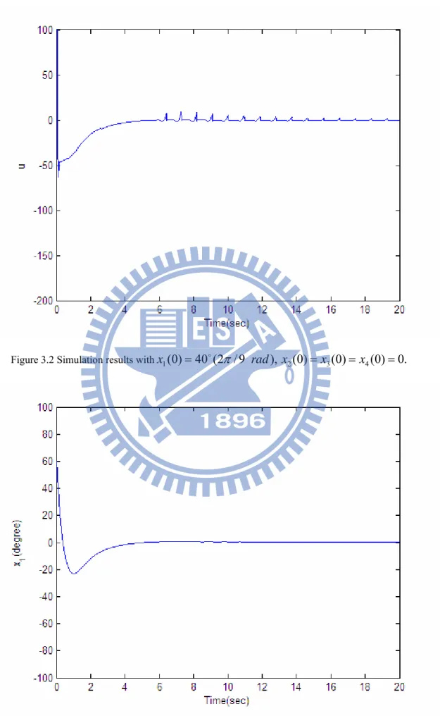
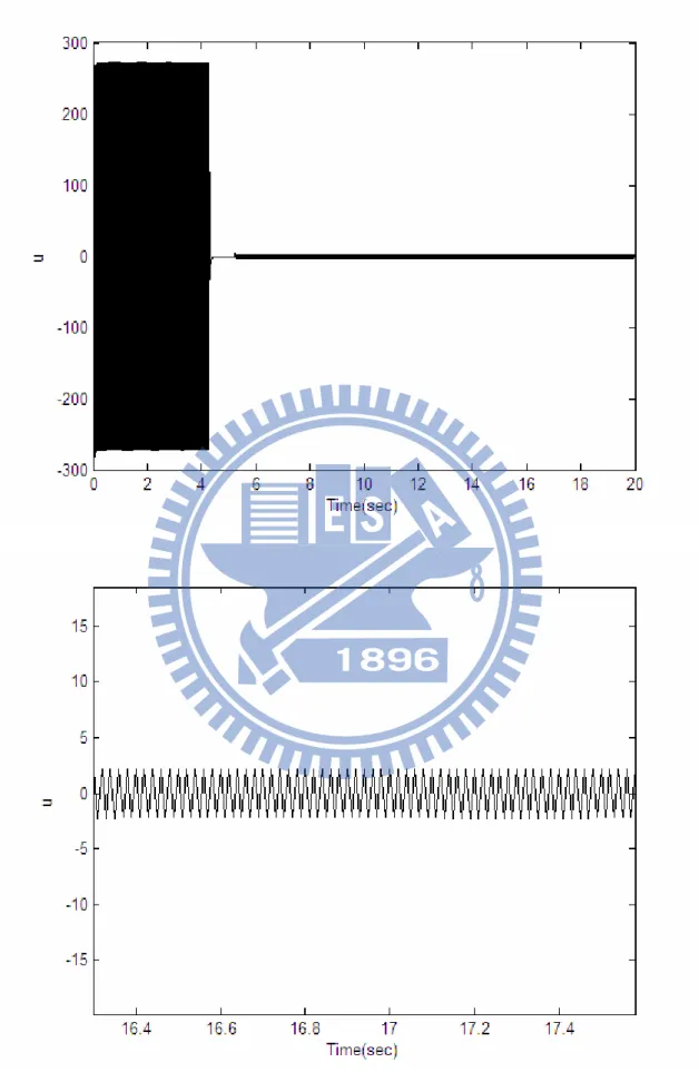
Figure 3.2 Simulation results withx₁(0)=40o(2π/9 rad), x₂(0)=x₃(0)=x₄(0)=0.33

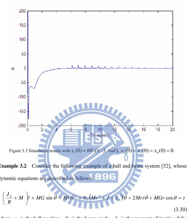
Figure 3.3 Simulation results withx₁(0)=60o(π/3 rad),x₂(0)=x₃(0)=x₄(0)=0. 36

Figure 3.4 Simulation results withx₁(0)=0.5,x₂(0)=x₃(0)=x₄(0)=0, including

amplifying the inputuscale...42

Figure 3.5 Simulation results with x₁(0)=1,x₂(0)=x₃(0)=x₄(0)=0, including amplifying the inputuscale...45

Figure 3.6 Simulation results withx₁(0)=x₂(0)=x₄(0)=0, x₃(0)=10...58

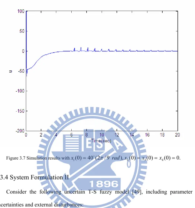
Figure 3.7 Simulation results withx₁(0)=40o(2π/9 rad),x₂(0)=x₃(0)= x₄(0)=0.64 Figure 3.8 Simulation results withx₁(0)= x₂(0)= x₄(0)=0, x₃(0)=10...79

Figure 3.9 Simulation results withx₁(0)=60o(π/3 rad),x₂(0)=x₃(0)=x₄(0)=0..84 Figure 3.10 Control results for the system (3.108) ...94

Figure 3.11 Simulation results with the proposed method on the two-rule T-S fuzzy model (3.110). ...100

Figure 3.12 Simulation results with the proposed method on the nonlinear truth model (3.109)...103

Figure 4.1 Simulation results withx₁(0)=20o(π/9 rad),x₂(0)=x₃(0)=x₄(0)=0..120 Figure 4.2 Simulation results withx₁(0)=40o(2π/9 rad),x₂(0)=x₃(0)=x₄(0)=0..124 Figure 4.3 Simulation results withx₁(0)=60o(π/3 rad),x₂(0)=x₃(0)=x₄(0)=0..128 Figure 4.4 Simulation results with x₁(0)=0.5,x₂(0)=x₃(0)=x₄(0)=0, including amplifying the inputuscale...135

Figure 4.5 Simulation results with x₁(0)=1,x₂(0)=x₃(0)=x₄(0)=0 , including amplifying the inputuscale...140

Figure 4.7 Simulation results withx1(0)=40o(2π/9rad),x2(0)=x3(0)=x4(0)=0...162

Figure 4.9 Simulation results withx₁(0)=60o(2π/9 rad), x₂(0)=x₃(0)=x₄(0)=0.185 Figure 4.10 Control results for the system (4.117). ...195

(10)

vi

Symbol List

) ( ), ( ), (t x t u t

ψ initial condition, state, and control input

i i i A B

A, _τ , state matrices, delayed state matrices, and input

matrices ) ( , , , ,µ β θ

θ_j _ij s r _i premise variables, fuzzy sets, number of premise

variables, number of IF-THEN rules, and membership function k k x t h x t

h( , ), ˆ( , ),ρ ,ρˆ unknown function, estimate ofh( xt, ), constants,

and estimate ofρ_k

g

E

S,σ, linear sliding surface parameter matrix, linear

sliding surface, and Lyapunov function

i

A

α

κ,Λ, κ =λ_min(BTB), any full rank matrix such that TΛ=0

B andΛTΛ=I , and known constant η δ, , , , ,c₀ c₁ c₂ Y decision variables ) ( , t

T_i Π_i constant matrix and time-varying matrix

m

d t

d_τ( ),τ, time-delay unknown function and known

constants. ) , , , ( ), ( , ), (t A A t h t x x u

x_d ∆ _i ∆ _τ_i _i _d delayed state, parameter uncertainties inA , _i

parameter uncertainties inA_τ_i, and external

disturbances

i i t φ

ξ ( ), known function and known constant

i m ε φ , known constants i i Z X K, , decision variables sampling dk dk dk dk,δ ,ρˆ ,δˆ ,t

ρ constants, estimate ofρ_dk,δ_dk, and sampling time

(11)

Chapter 1 Introduction

Up to now, fuzzy systems have been applied with great success to numerous real world applications, such as Penicillin-G conversion [1], prediction of river water flow [2], and many other examples in ecological systems and biomedical field [1], [3]. In the meantime, numerous publications have been reported in providing theoretical support. Various methodologies have been proposed for analysis, modeling, design, control and monitor of fuzzy systems. Fuzzy ideas are useful for modeling complex nonlinear systems in which, due to the complexity or the uncertainty, classical tools are unsuccessful. The truth model is too complicated for use in the controller design. Thus, we need to develop a simplified model that can be used to design a controller. Such a simplified model is labeled by Friedland [4] as the design model. The design model should capture the essential features of the process. In practice, the inevitable uncertainties may enter a nonlinear system model in a very complicated way. The uncertainty may include modeling errors, parameter variations, external disturbances, and fuzzy approximation errors. In such a situation, some fuzzy feedback control design methods may not work well anymore. To deal with the problem, this dissertation provides two kinds of LMI-based robust adaptive sliding control, including a sliding control method and an adaptive control method.

The introduction of this dissertation is introduced in this chapter. The motivation of this dissertation is discussed in Section 1.1. In Section 1.2, related works are introduced. The approach of this dissertation is described in Section 1.3. In Section 1.4, the organization of the dissertation is introduced.

(12)

2

1.1 Motivation

The first step in the controller design procedure is the construction of a “truth model” of the dynamics of the process to be controlled. The truth model is a simulation model that includes all the relevant characteristics of the process. The truth model is too complicated for use in the controller design. Thus, we need to develop a simplified model that can be used to design a controller. Such a simplified model is labeled by Friedland [4] as the design model. The design model should capture the essential features of the process. In many situations, there may be human experts who can provide a linguistic description of the process in terms of IF-THEN rules. Combining the available mathematical description of the process with its linguistic description results in a fuzzy system model. Such an approach to modeling was proposed by Takagi and Sugeno [5] and further developed by Sugeno and Kang [6]. This type of model is called the Takagi-Sugeno (T-S) or Takagi-Sugeno-Kang (TSK) fuzzy model.

T-S fuzzy models are popular and well used tools in recent years. A general T-S fuzzy model employs an affine fuzzy model with a constant in the consequence [5]. It is known that smooth nonlinear dynamic systems can be approximated by affine T-S fuzzy models [7,8]. Most recent developments are based on T-S models with linear rule consequences (here and after, such models are generally called T-S fuzzy models). The main feature of T-S fuzzy models is to represent the nonlinear dynamics by simple (usually linear) models according to the so-called fuzzy rules and then to blend all the simple models into an overall single model through nonlinear fuzzy membership functions. Each simple model is called a local model or a sub-model. The output of the overall fuzzy model is calculated as a gradual activation of the local models by using proper defuzzification schemes [5], [9,10]. It has been proved that T-S fuzzy models can approximate any smooth nonlinear dynamic systems [11,12]. Based on the sector

(13)

nonlinearity concept [12], the uncertain nonlinear system can be systematically constructed by T–S fuzzy models.

In practice, the inevitable uncertainties may enter a nonlinear system model in a very complicated way. The uncertainty may include modeling errors, parameter variations, external disturbances, and fuzzy approximation errors. In such a situation, some fuzzy feedback control design methods may not work well anymore.

On the other hand, time-delay is often encountered in various industrial systems, such as the turbojet engine, electrical networks, nuclear reactor, rolling mill, and chemical process, etc. Recently, the feedback stabilization problem for uncertain time-delay systems is also a problem of interest because the existence of a delay is frequently a source of poor system performance or instability. However, they are sensitive to the uncertainty, which directly affects the control systems.

1.2 Related Works

The history of the so-called parallel distributed compensation (PDC) began with a model-based design procedure proposed by [13]. However, the stability of the control systems was not addressed in the design procedure. The design procedure was improved and the stability of the control systems was analyzed in [14]. The design procedure is named “parallel distributed compensation” in [15]. The PDC [14-16] offers a procedure to design a fuzzy controller from a given T-S fuzzy model. It should be noted that many real systems, for example, mechanical systems and chaotic systems, can be and have been represented by T-S fuzzy models.

It is well-known that time-delay is a common and complex phenomenon in many industrial and engineering systems, such as communication systems, rolling mill systems and transportation systems. Since 2000, the T-S fuzzy model has been extended

(14)

4

recently, great progress has been made in the analysis and synthesis of T-S fuzzy systems with time-delay, such as stability and stabilization based on the parallel distributed compensation (PDC) method [17-19].

On H_∞control, the problem of static output feedback control was developed in

[20,21]. Robust stability and guaranteed cost control were treated in [22]. Chen and Liu [21] proposed a robustH_∞control by using the Lyapunov-Krasovskii function (LKF)

∫

∫ ∫

− + − + + = t t t t t T T T dsd s x R s x ds s x Q s x t Px t x t x V ) ( 0 ) ( ) ( ) ( ) ( ) ( ) ( )) ( ( τ τ η & & η

and model transformation technique which introduced conservatism.

1.3 Approach

Over the past two decades, fuzzy techniques have been widely and successfully exploited in nonlinear system modeling and control. The Takagi-Sugeno (T-S) model [5] is a popular and convenient tool for handling complex nonlinear systems. Correspondingly, the fuzzy feedback control design problem for a nonlinear system has been studied extensively by using T-S model where simple local linear models are combined to describe the global behavior of the nonlinear system [23-29]. In practice, the inevitable uncertainties may enter a nonlinear system model in a very complicated way. The uncertainty may include modeling errors, parameter variations, external disturbances, and fuzzy approximation errors. In such a situation, the fuzzy feedback control design methods of [23-29] may not work well anymore. To deal with the problem, some authors [30,31] have exploited the variable structure system (VSS) theory which has provided an effective means to design robust controllers for uncertain nonlinear systems where the uncertainties are bounded by known scalar valued functions.

(15)

viable high-speed switching feedback control to obtain a desired system response, from which the VSS arises in finite time. The VSS drives the trajectory of the system onto a specified and user-design surface, which is called the sliding surface or the switching surface, and maintains the trajectory on this sliding surface for all subsequent time. The closed-loop response obtained from using a VSS control law comprises two distinct modes. The first is the reaching mode, also called nonsliding mode, in which the trajectory starting from anywhere on the state space is being driven towards the switching surface. The second is the sliding mode in which the trajectory asymptotically tends to the origin. The central feature of the VSS is the sliding mode on the sliding surface on which the system remains insensitive to internal parameter variations and external disturbance. In sliding mode, the order of the system dynamics is reduced. This enables simplification and decoupling design procedure [32-35]. However, all the VSS-based fuzzy control system design methods are based on the assumption that each nominal local system model shares the same input channel. This assumption is very restrictive and inadequate to modeling uncertainty/nonlinearity in various mechanical systems such as an inverted pendulum on a cart.

Some authors [36-40] have relaxed the assumption and they have proposed adaptive laws to estimate the upper norm bounds. However, the previous VSC-based fuzzy control methods have considered the problem of adaptive control design and stability analysis for uncertain T-S fuzzy models where the input matrices of the local system models satisfy the assumption that each nominal local system shares the same input channel. It is practically difficult to satisfy this assumption.

On the other hand, time-delay is often encountered in various industrial systems, such as the turbojet engine, electrical networks, nuclear reactor, rolling mill, and chemical process, etc. Recently, the feedback stabilization problem for uncertain

(16)

6

time-delay systems is also a problem of interest because the existence of a delay is frequently a source of poor system performance or instability [41-43]. However, they are sensitive to the uncertainty, which directly affects the control systems.These years, other authors [44-46] have exploited the SMC approach theory which has provided an effective means to design robust controllers for uncertain fuzzy time-delay systems where external disturbances are bounded by known upper norm bounds.

In this dissertation, we propose two kinds of LMI-based robust adaptive sliding control, including a robust sliding control method and a robust adaptive control method, for uncertain Takagi-Sugeno fuzzy models with norm-bounded uncertainties, and meantime relax the restrictive assumption that each nominal local system model shares the same input channel, which is required in the traditional VSS-based fuzzy control design methods. Then, two kinds of LMI-based robust adaptive sliding control are developed for uncertain T-S fuzzy models which include mismatched parameter uncertainties and external disturbances. Moreover, two kinds of LMI-based robust adaptive sliding control are proposed for the uncertain T-S fuzzy time-delay model which includes mismatched parameter uncertainties in the state matrix and norm-bounded external disturbances. Finally, some examples are used to illustrate the effectiveness and usefulness of the proposed methods for distinct uncertain T-S fuzzy models and to compare with the existing methods in each final subsection.

1.4 Organization of this Dissertation

This dissertation comprises five chapters. In Chapter 1, the introduction comprises motivation, related works, approach, and organization of this dissertation. In Chapter 2, foundations are described by providing concepts of Lyapunov stability and linear matrix inequality. In Chapter 3, LMI-based robust sliding control design methods are developed for different uncertain Takagi-Sugeno fuzzy models with

(17)

matched/mismatched parameter uncertainties and external disturbances which are bounded by known scalar valued functions and meantime we relaxed the restrictive assumption that each nominal local system model shares the same input channel, which is required in the traditional VSS-based fuzzy control design methods. Besides, a robust sliding control design method is also presented for the uncertain T-S time-delay model with mismatched parameter uncertainties and external disturbances. Finally, some examples are used to illustrate the effectiveness of the proposed methods for distinct uncertain T-S fuzzy models and to compare with the existing methods in each final subsection. In Chapter 4, LMI-based robust adaptive control design methods are proposed for distinct uncertain T-S fuzzy models which include matched/mismatched parameter uncertainties and unknown norm-bounded external disturbances. Moreover, a robust adaptive control design method is also proposed for the uncertain T-S time-delay model with mismatched parameter uncertainties and external disturbances. Finally, some examples are used to illustrate the effectiveness of the proposed methods for distinct uncertain T-S fuzzy models and to compare with the existing methods in each final subsection. In Chapter 5, the contributions are discussed and suggestions for future work are proposed.

(18)

8

Chapter 2 Foundations

In this chapter, the basic concepts that relate to the proposed control methods are introduced. The Lyapunov stability is discussed in the first section. Section 2.2 introduces the concept of linear matrix inequality (LMI).

2.1 Lyapunov Stability

Consider a general nonlinear system [47]

x&=A(x) (2.1)

where n

R

x∈ are the state variables and A:Rn →Rnis a nonlinear function. We assume

that A is such that system (2.1) has a unique solution x(t) over [0,∞ for all initial ) conditions x(0) and that the solution depends continuously on x(0) . A vector

n

R

x₀∈ is an equilibrium point of the system (2.1) ifA(x₀)=0.

Without loss of generality, we can assume that x₀ =0 is an equilibrium point of the system (2.1); that is, A(0)=0. Otherwise, we can perform a simple state transformation z= x−x₀ to obtain a new state equation z&= A~(z)= A(z+x₀) where

0 0 =

z is an equilibrium point, that is, A~(0)=A(x₀)=0.Clearly, the solution of the

differential equation (2.1) shows that if x(0)=0, then x(t)=0, for all t>0 .

However, this solution may or may not be stable.

Definition 2.1.1:

Stability: The equilibrium point x₀ =0 of the system (2.1) is stable if for all ε >0, there exists a δ(ε) > 0 such that x(0) < δ(ε)⇒ x(t) < ε , ∀t≥0.

(19)

In other words, the equilibrium point x₀ =0 is stable if arbitrarily small perturbations of the initial state x(0)=0 from the equilibrium point result in arbitrarily small perturbation of the corresponding state trajectoryx(t).

Definition 2.1.2:

Asymptotic Stability: The equilibrium point x₀ =0 of the system (2.1) is asymptotically stable if it is stable and there exists some γ >0 such that if x(0) <γ ,

thenx(t)→0 as t→∞.

In other words, the equilibrium point x₀ =0 is asymptotically stable if there exists a neighborhood of x₀ =0 such that if the system starts in the neighborhood, then its trajectory converges to the equilibrium point x₀ =0 as t→∞.

The equilibrium point x₀ =0 of the system (2.1) is globally asymptotically stable if γ >0 can be arbitrarily large; that is, all trajectories converges to the equilibrium point 0x₀ = .

Determining stability of a system may not be an easy task if the system is nonlinear. One approach often used to determine stability is that of Lyapunov. Intuitively, the Lyapunov stability theorem can be explained as follows. Given a system with an equilibrium point x₀ =0, let us define some suitable “energy” function of the system. The function must have the property that is zero at an equilibrium point x₀ =0 and positive elsewhere. Assume further that the dynamic system is such that the energy of the system is monotonically decreasing with time and hence eventually reduces to zero. Then, the trajectories of the system have no other places to go but the origin. Therefore, the system is asymptotically stable. This generalized energy function is called a Lyapunov function. If there exists a Lyapunov function, then we can prove the

(20)

10

asymptotic stability using the following Lyapunov stability theorem.

Theorem 2.1.1

The equilibrium point x₀ =0 of the system (2.1) is asymptotically stable if there exists a Lyapunov function V :Rn →R such that V(x)>0 , x≠0 , V(x)=0 ,

0 =

x ,V&(x)<0, and x≠0, 0V&(x)= ,x=0 is true in a neighborhood of x₀ =0,

{

<γ

}

= x x

N : for some γ >0.

Proof:

We provide the following intuitive proof by contradiction. If the equilibrium point 0

0 =

x of the system (2.1) is not asymptotically stable; that is, x(t)→0 as t→∞ is

not true even if x(0) <γ for some γ >0, then V&(x)<−α for some α >0. Since

∫

= +

∫

− = − + =V x tV x d V x t d V x t t x V 0 ( ) ( (0)) 0 ( (0)) )) 0 ( ( )) ( ( & τ α τ α .

For a sufficiently large t , 0V(x(t))< . This contradicts the assumption V(x(t))≥0.

The key to proving stability of a system using the Lyapunov stability theorem is to construct a Lyapunov function. This construction must be done in a case-by-case basis. There is no general method for the construction. The following example illustrates the application of the Lyapunov stability theorem.

Example 2.1.1

Let us consider the following system:

1 2

1 x 3x

x& = − , x&₂ =−x₂3−2x₁.

To prove it is asymptotically stable, let us consider the following Lyapunov function: 2 2 2 1 2 ) (x x x V = + . Clearly,V(x)>0, x≠0, V(x)=0, x=0.

(21)

On the other hand, 2 2 1 1 2 4 ) (x x x x x

V& = & + & =4x₁(x₂−3x₁)+2x₂(−x₂3−2x₁)

2 1 4 2 2 1 2 1 12 2 4 4xx − x − x − xx = 4 2 2 1 2 12x − x − = .

Therefore,V&(x)<0, x≠0,V&(x)=0, x=0.

Finally, we can conclude that the system is asymptotically stable.

2.2 Linear Matrix Inequality

A linear matrix inequality (LMI) has the form [48]

0 ) ( 1 0+ > ≡

∑

= m i i iF x F x F (2.2) where m R

x∈ is the variable and the symmetric matrices F_i =F_iT ∈Rn×n, i=0,...,m,

are given. The inequality symbol in (2.2) means that F(x) is positive-definite, i.e., 0

) (x u >

F

uT for all nonzero u∈Rn. Thus, the LMI (2.2) is equivalent to a set of n

polynomial inequalities inx, i.e., the leading principal minors of F(x) must be

positive. We will also encounter nonstrict LMIs, which have the form 0

) (x ≥

F . (2.3)

The strict LMI (2.2) and the nonstrict LMI (2.3) are closely related.

The LMI (2.2) is a convex constraint onx, i.e., the set {x|F(x)>0}is convex.

Though the LMI (2.2) may seem to have a specialized form, it can represent a wide variety of convex constraints on x . In particular, linear inequalities, quadratic

inequalities, matrix norm inequalities, and constraints that arise in control theory, such as Lyapunov and convex quadratic matrix inequalities, can all be cast in the form of an LMI.

Multiple LMIs (1)( )_>0

x

(22)

12 0 )) ( , ), ( ( (1) _⋅_⋅_⋅ ( ) _> x F x F

diag p . Therefore we will make no distinction between a set of

LMIs and single LMI, i.e., “the LMI (1)( )_>0

x

F ,⋅ ⋅⋅, F(p)(x)>0” will mean “the LMI

0 )) ( , ), ( ( (1) _⋅_⋅_⋅ ( ) _> x F x F diag p ”.

When the matricesF are diagonal, the LMI i F(x)>0 is just a set of linear

inequalities. Nonlinear (convex) inequalities are converted to LMI form using Schur complements. The basic idea is as follows: the LMI

0 ) ( ) ( ) ( ) ( >       x R x s x S x Q T (2.4) where T x Q x

Q( )= ( ) , R(x)=R(x)T, and S(x)depend affinely on x, is equivalent to

0 ) (x >

R , 0Q(x)−S(x)R(x)−1S(x)T > . (2.5)

In other words, the set of nonlinear inequalities (2.5) can be represented as the LMI (2.4).

As an example, the matrix norm constraint Z(x) <1, where Z(x)∈Rp×qand

depends affinely on x, is represented as the LMI

0 ) ( ) ( >       I x Z x Z I T Since Z <1 is equivalent to I −ZZT >0.

We will often encounter problems in which the variables are matrices, e.g., the Lyapunov inequality 0 < + PA P AT _(2.6) where n n R

A∈ × is given and P=PTis the variable. In this case we will not write out the

LMI explicitly in the formF(x)>0, but instead make clear which matrices are the variables. The phrase “the LMIATP+ PA<0in P ” means that the matrix P is a variable. Of course, the Lyapunov inequality (2.6) is readily put in the form (2.2), as

(23)

follows. LetP₁,⋅ ⋅⋅, P be a basis for symmetric m n×n matrices. Then take F0 =0 and A P P A F i i T

i =− − . Leaving LMIs in a condensed form such as (2.6), in addition to

saving notation, may lead to more efficient computation.

As another related example, consider the quadratic matrix inequality 0 1 ₊ _< + + − Q P B PBR PA P AT T (2.7) where A , B , T Q

Q= , R=RT >0 are given matrices of appropriate sizes,

and T

P

P= is the variable. Note that this is a quadratic matrix inequality in the

variable P . It can be expressed as the linear matrix inequality

0 >      − − − R P B PB Q PA P A T T .

This representation also clearly shows that the quadratic matrix inequality (2.7) is convex in P , which is not obvious.

Finally, given an LMI F(x)>0, the corresponding LMI Problem (LMIP) is to find feas

x such that F(xfeas)>0 or determine that the LMI is infeasible. Of course,

this is a convex feasibility problem. We will say “solving the LMIF(x)>0” to mean solving the corresponding LMIP.

As an example of an LMIP, consider the “simultaneous Lyapunov stability problem”: We are given n n

i R

A ∈ × , i=1,⋅ ⋅⋅,L,and need to find P satisfying the LMI

0 >

P , A_iTP+ PA_i <0, i=1,⋅ ⋅⋅,L

(24)

14

Chapter 3 LMI-Based Robust Sliding Control

In this chapter, LMI-based robust sliding control methods are developed for different uncertain Takagi-Sugeno fuzzy models/time-delay models. The introduction of this chapter is introduced in Section 3.1. In Section 3.2, a robust sliding control method is proposed for T-S fuzzy systems. Section 3.3 presents two kinds of robust sliding control methods for mismatched T-S fuzzy systems. A robust sliding control method is presented for mismatched T-S fuzzy time-delay systems in Section 3.4.

3.1 Introduction

Over the past two decades, fuzzy techniques have been widely and successfully exploited in nonlinear system modeling and control. The Takagi-Sugeno (T-S) model [5] is a popular and convenient tool for handling complex nonlinear systems. Correspondingly, the fuzzy feedback control design problem for a nonlinear system has been studied extensively by using T-S model where simple local linear models are combined to describe the global behavior of the nonlinear system [23-29]. In practice, the inevitable uncertainties may enter a nonlinear system model in a very complicated way. The uncertainty may include modeling errors, parameter variations, external disturbances, and fuzzy approximation errors. In such a situation, the fuzzy feedback control design methods of [23-29] may not work well anymore. To deal with the problem, some authors [30,31] have exploited the variable structure system (VSS) theory which has provided an effective means to design robust controllers for uncertain nonlinear systems where the uncertainties are bounded by known scalar valued functions.

(25)

In the VSS, the control design of the plant is intentionally changed by using a viable high-speed switching feedback control to obtain a desired system response, from which the VSS arises in finite time. The VSS drives the trajectory of the system onto a specified and user-design surface, which is called the sliding surface or the switching surface, and maintains the trajectory on this sliding surface for all subsequent time. The closed-loop response obtained from using a VSS control law comprises two distinct modes. The first is the reaching mode, also called nonsliding mode, in which the trajectory starting from anywhere on the state space is being driven towards the switching surface. The second is the sliding mode in which the trajectory asymptotically tends to the origin. The central feature of the VSS is the sliding mode on the sliding surface on which the system remains insensitive to internal parameter variations and external disturbance. In sliding mode, the order of the system dynamics is reduced. This enables simplification and decoupling design procedure [32-35]. However, all the VSS-based fuzzy control system design methods are based on the assumption that each nominal local system model shares the same input channel. This assumption is very restrictive and inadequate to modeling uncertainty/nonlinearity in various mechanical systems such as an inverted pendulum on a cart.

On the other hand, time-delay is often encountered in various industrial systems, such as the turbojet engine, electrical networks, nuclear reactor, rolling mill, and chemical process, etc. Recently, the feedback stabilization problem for uncertain time-delay systems is also a problem of interest because the existence of a delay is frequently a source of poor system performance or instability [41-43]. However, they are sensitive to the uncertainty, which directly affects the control systems.

In this chapter, we propose robust sliding control design methods for different uncertain T-S fuzzy models with matched/mismatched parameter uncertainties and

(26)

16

external disturbances which are bounded by known scalar valued functions. Each nominal local system model of the uncertain system under consideration may not share the same input channel. As the local controller, we use a sliding mode controller with a nonlinear switching feedback control term. We derive LMI conditions for existence of linear sliding surfaces guaranteeing asymptotic stability of the reduced order equivalent sliding mode dynamics, and we give an explicit formula of the switching surface parameter matrix in terms of the solution of the LMI existence conditions. The nonlinear switching feedback control term is also designed to drive the system trajectories so that a stable sliding motion is induced in finite time on the switching surface and the state converges to zero. Besides, a robust sliding control design method is also presented for the uncertain T-S time-delay model with mismatched parameter uncertainties and external disturbances. Finally, some examples are used to illustrate the effectiveness of the proposed methods for distinct uncertain T-S fuzzy models and to compare with the existing methods in each final subsection.

3.2 Robust Sliding Control for T-S Fuzzy Systems

In this section, system formulation for the uncertain T-S fuzzy model is described in Section 3.2.1. A robust sliding control method via LMI is proposed in Section 3.2.2. Some examples are used to illustrate the effectiveness of the proposed methods and to compare with the existing methods in Section 3.2.3.

3.2.1 System Formulation

Consider the following uncertain T-S fuzzy model [49]:

[

( ) ( ) ( , )

]

) ( ) ( 1 x t h B t u B t x A t x _i _i _i r i i + + =

∑

= θ β & (3.1) where n R t

(27)

matrices of appropriate dimensions, θ =[θ₁,⋅⋅⋅,θs],θj(j =1,⋅⋅⋅,s) are the premise variables, s is the number of the premise variables, βi(θ)=

∑

= r

j j

i(θ)/ ₁ω (θ),

ω ωi :Rs →[0,1],i =1, ⋅⋅⋅,ris the membership function of the system

with respect to plant rule ri, is the number of the IF-THEN rules, β_i can be regarded

as the normalized weight of each IF-THEN rule and it satisfies

that βi(θ)≥0,

∑

₌₁β (θ)=1, r i i m R x t

h(, )∈ stands for the lumped nonlinearities or

uncertainties. We will assume that the followings are satisfied:

A1: The n×m matrix B defined by =

∑

r_i₌ Bi

r

B 1 ₁ satisfies the rank constraint

rank(B)=m, i.e., the matrix B has full column rankm.

A2: The function h( xt, ) is unknown but bounded as k

l k k x x t h x t h

∑

= ≤ − 0 ) , ( ˆ ) , ( ρ

where ρ₀,⋅ ⋅⋅,ρ_lare known constants, hˆ x(t, )is an estimate of h( xt, ), and lis a

known positive integer.

The system (3.1) does not have to satisfy the restrictive assumption that all the input matrices of the local system models are in the same range space. It should be noted that the assumption A1 implies that rank(B_i)≤mand each nominal local system model

may not share the same input channel. The assumption A2 with l=1 and

0 ) , ( ˆ _t _x ₌

h has been used in the literature [50]. We can set hˆ x(t, )as the nominal value

of h( xt, ).Using the above assumptions, the uncertain T-S fuzzy model (3.1) can be written as follows. )] , ( ][ ) ( [ ) ( ) ( ) ( 1 x t h u G HF B t x A t x i r i i + + + =

∑

= β θ β & (3.2)

(28)

18

[

( ), ,( )

]

, 2 1 1 B Br B B H = − ⋅ ⋅⋅ − G=

[

I,⋅ ⋅⋅,I

]

T,

[

(1 2 ( )) , ,(1 2 ( ))

]

. ) ( diag ₁ I I F β = − β θ ⋅ ⋅⋅ − β_r θ (3.3)

It should be noted that the system (3.1) does not have to satisfy

,

2

1 B Br

B = =⋅ ⋅⋅= which is used in almost all published results on VSS design methods

including the VSS-based fuzzy control design methods of [33,34]. Hence the methods [30,31] cannot be applied to the above model (3.1). Since β_i(θ)≥0 and

∑

= =

r

i 1β(θ) 1,we can see that the following inequality always holds:

. ) ( ) ( ) ( ) ( F F F I FT β β = β T β ≤ (3.4)

Many examples in the literature and various mechanical systems such as motors and robots do not satisfy the restrictive assumptions that each nominal local system model shares the same input channel and they fall into the special cases of the above model [49].

3.2.2 Sliding Control Design via LMI

The Sliding Mode Control (SMC) design is decoupled into two independent tasks of lower dimensions: The first involves the design of m(n− )1 −dimensional switching surfaces for the sliding mode such that the reduced order sliding mode dynamics satisfies the design specifications such as stabilization, tracking, regulation, etc. The second is concerned with the selection of a switching feedback control for the reaching mode so that it can drive the system’s dynamics into the switching surface [33]. We first characterize linear sliding surfaces using LMIs.

Let us define the linear sliding surface as σ = xS = 0where Sis a m×nmatrix.

Referring to the previous results [33], [51], we can see that for the system (3.2) it is reasonable to find a sliding surface such that

(29)

P1

[

SB+SHF(β)G

]

is nonsingular for any β satisfying βi(θ)≥0,i=1,⋅ ⋅⋅,r, and

∑

= =

r

i 1βi(θ) 1.

P2 The reduced (n−m)order sliding mode dynamics restricted to the sliding surface 0

=

x

S is asymptotically stable for all admissible uncertainties.

It should be noted that P1 is necessary for the existence of the unique equivalent control [33] and the assumption A1 is necessary for the nonsingularity of SB.

Define a transformation matrix and the associated vector vas M=[Λ(ΛTYΛ)−1,

T T B Y B B Y−1 ( −1 )−1] [ T, T]T, S V = v=[v₁T,vT₂]T =Mx where v₁∈Rn−m ,v₂∈Rm. By the

above transformation, we can see that 1 [ , ]

B Y

M− = Λ and v₂ =σ. Then, from system

(3.2), we can obtain             Λ Λ =      

∑

= σ θ β σ 1 1 1 ₍ ₎ v B SA Y SA B VA Y VA v r i i i i i i & & _[ ₍ _, _)]. ) ( ) ( x t h u G SHF I G VHF +       + + β β (3.5)

From the equivalent control method [33], we can see that the equivalent control is

given by ueq(t)= ( )[ ( ) ] (, ). 1 1 I SHF G SAix h t x r i i + − − − =

∑

β θ β By setting σ_& =σ =0and

substituting u(t)with u_eq(t),we can obtain that the reduced (n−m)order sliding

mode dynamics restricted to the switching surface σ = Sx=0is given by 1 1 1 1 ( )( Y ) D( )AY v v i T r i T i Λ Λ Λ Λ =

∑

= − _β θ β & (3.6) where ( ) ( ) [ ( ) ] 1 . S G SHF I G HF I D β = − β + β −

Theorem 3.1 Let us consider the sliding mode dynamics (3.6). If there exist

matrices n n, R Y∈ × Λ∈Rn×(n−m)satisfying ,BTΛ =0,ΛTΛ=I scalarsc₁∈R,c₂∈R,η∈R, ), ( min B B T λ

κ = and ∗ represents blocks that are readily inferred by symmetry such that the following LMIs holds:

(30)

20 i I H Y A I H Y A i T i T ∀ <           − Λ ∗ − Λ ∗ ∗ Λ ∗ + Λ , 0 ) ( η η (3.7) , 0 0 0 0 0 2 1 >           − Y I c I c I I Y (3.8) 0 0 0 2 2 1 >           ∗ ∗ η η ηκ r rc r rc (3.9)

then, there exists a linear sliding surface parameter matrix Ssatisfying P1-P2 and the

sliding surface 0 ) ( ) ( ₌ ₌ −1 −1 −1 ₌ x Y B B Y B x S x T T σ (3.10)

will guarantee that the sliding mode dynamics (3.6) is asymptotically stable.

Proof: By using Schur complement formula [48], we can easily show that in fact the

following LMIs are incorporated in the LMIs (3.7)-(3.9)

, , 0 , 0 , 0 2 2 1 c HH I c > > η> η T < 2η2κ >r(c₁2 +c₂2). (3.11)

It is clear that if the following inequality (3.12) holds, then SB+SHF(β)G G

SHF I+ (β)

= is nonsingular and hence P1 holds

. ) ( ) ( GG F H S I SHF β T T β T T < (3.12)

Using (3.3), (3.4), (3.11) and GGT ≤ G 2I =rI, we can obtain . ) ( ) ( T T T T ₂ T SS r S H F GG SHF η β β ≤ (3.13) By using the Schur complement formula, we can see that (3.8) and (3.11) imply

, 0 1 ₂ 1 I Y c I c < < < − I c Y I c₂1 1 ₁ 0< − < − < (3.14) and this leads to

(31)

T T T T T SS r S H F GG SHF( ) ( ) ₂ η β β ≤ ( ) 1 1₂2 . 2 2 1c _B _B rcc _I rc T κη η ≤ ≤ − _(3.15)

Using the inequality ₂ 2 2

b a

ab≤ + wherea and bare scalars, we can show that (3.15)

implies . ) ( 2 ) ( ) ( 2 2 2 1 2 c c I r S H F GG SHF T T T T ≤ + κη β β (3.16)

Finally, by using the above inequalities (3.11) and (3.16), we can obtain

I SS r S H F GG SHF( ) T T( ) T T ≤ ₂ T < η β β (3.17)

which implies that [SB+SHF(β)G]is nonsingular, i.e., P1 holds.

Now, we will show that Sof (3.10) guarantees P2. Using the matrix inversion lemma: B BA I A I AB I ) 1 ( ) 1 ( ₊ − ₌ ₋ ₊ −

where A and B are compatible constant matrices such that (I+AB)is nonsingular, we can show that the sliding mode dynamics (3.6) is equivalent to

∑

= − _Λ _Λ Λ Λ = r i i T T i Y C AY v v 1 1 1 1 β (θ)( ) (β) & (3.18) where ₍ ₎₌ ₋ _[ ₊ ₍ ₎ _]−1 ₍ ₎ ₌_[ ₊ ₍ ₎ _]−1 GS HF I GS F GSH F I H I C β β β β ). ( ] ) ( [ ) (_β _β 1 _β D S G SHF I G HF I− + = = −

The sliding mode dynamics (3.18) is asymptotically stable if there exists a positive

definite matrix ( )( ) 0 m n m n R

P ∈ − × − such that the time derivative of the Lyapunov function

1 0 1

)

(t v Pv

E_g = T satisfies for some positive scalarτ

∑

= − ≤ Ζ = r i T i T i g t v P v v v E 1 1 0 1 1 1 ) ( ) ( 2 ) ( β θ β τ & (3.19) where ( ) ( [ ( ) ] 1 ( ) ₀) 0 0 0 i i i β A B I N β D N β C − − + = Ζ , Λ Λ Λ Λ = − Y A Y A i T T i 1 0 ( ) ,B Y H T T Λ Λ Λ = −1 0 ( ) ,Ci 0 = YAi Λ, D0 =H, N(β)=−F(β)GS.

(32)

22

It should be noted that the inequalities (3.4), (3.11), (3.17) andGGT ≤ G 2I =rI imply

, ) ( ) ( ) ( ) ( 2 I F G GSS F N N β T β = β T T T β ≤η η2D₀TD₀ =η2HTH <I (3.20)

This and (3.19) imply that (3.18) is asymptotically stable if there exists a positive definite matrixP such that ₀

0 ) ( ] ) ( [ 1 ₀ 0 0 0 0 0 + − Ν +∗< − i i P B I N D C A P β β , ∀i (3.21)

where ∗ represents blocks that are readily inferred by symmetry.

Let z be i zi I N D N Ci0y 1 0] ( ) ) ( [ − β − β = where (n m) R y∈ − .

Then z can be rewritten as_i z_i =N(β)[C_i₀y+D₀z_i].

This equality and (3.20) imply 2[ ₀ ₀ ] [ ₀ ₀ ]

i i T i i i T i z C y D z C y D z

z ≤η + + and this leads to

y C D N I B P yT ₀ ₀[ ( ) ₀] 1 ( ) _i₀ 2 − β − Ν β i T i i i T i i i T i T z z z D y C z D y C z B P y z B P y ₀ ₀ 2 ₀ ₀ [ ₀ ₀ ] [ ₀ ₀ ] 2 2 ≤ + + + − − = η i T i i T i T i T i T z z z D C B P y y C C y + + − Ω = −2 0 0 0 0 0 0 2 [ ] η whereΩ=I−η2D0TD0. (3.22)

SinceΩ>0, the following inequality holds for any(y,zi):

y D C B P D C B P y z z z D C B P y iT T T i T i T i i T i T_[ _] _[ _] _[ _] 2 1 ₀ ₀ ₀ ₀ 0 0 0 0 2 2 0 0 0 0 + ≤ Ω + + Ω + − − _η η (3.23)

Using (3.22) and (3.23), we can show that the Lyapunov inequality (3.21) is satisfied if the following inequality holds:

0 ] [ ] [ 1 ₀ ₀ ₀ ₀ 0 0 0 0 2 0 0 0 0 0 0 + + + + Ω + < − T T i T i i T i T i i A P C C P B C D P B C D A P η .

Using the Schur complement formula, we can rewrite the above inequality as

0 0 0 0 0 0 <           − ∗ − ∗ ∗ ∗ + I D C I P B P A i T o T i η η , ∀i. (3.24)

(33)

Let the positive definite matrix P be₀ P₀ =ΛTYΛ where Y is a solution to LMIs

(3.7)-(3.9), which implies that the sliding mode dynamics (3.18) is asymptotically stable. Hence, the sliding mode dynamics (3.6) is asymptotically stable.

After the switching surface parameter matrix Sis designed so that the reduced

)

(n−m order sliding mode dynamics has a desired response, the next step of the SMC

design procedure is to design a switching feedback control law for the reaching mode such that the reachability condition is met. If the switching feedback control law satisfies the reachability condition, it drives the state trajectory to the switching surface

0 = = xS

σ and maintains it there for all subsequent time. With σ of (3.10), we design a sliding fuzzy control law guaranteeing that σ converges to zero. We will use the following nonlinear sliding switching feedback control law as the local controller.

Control rule i: IF θ is ₁ µ_i₁and ... and θ_sis µ_is, THEN

σ σ δ ω σ χ ( , ) 1 1 ) , ( ˆ ) (t h t x SA x t x u _i _i _i − − − − − = where l k k k i i i t x SA x

∑

x = + + + = 0 ) 1 ( ) , ( α ω ω ρ δ (3.25)

and σ =Sx,ω= r SH ,α_i >0,χ_i >0. It should be noted that (3.17) implies ω=

SH

r ≤ r S ⋅ H ≤η H .This and (3.11) guarantee 0≤ω <1. The final controller

inferred as the weighted average of the each local controller is given by

∑

=         − + + − − = r i i i i i SA x t x x t h t u 1 ) , ( 1 1 ) ( ) , ( ˆ ) ( σ σ δ ω σ χ θ β (3.26)

and we can establish the following theorem.

Theorem 3.2 Consider the closed-loop control system of the uncertain system

(34)

24

) , , ,

(Y c₁ c₂ η and the linear sliding surface is given by (3.10). Then the state converges

to zero.

Proof: Since Theorem 3.1 implies that the linear sliding surface (3.10) guarantees

P1-P2, we only have to show that σ converges to zero. Define a Lyapunov function as ( ) 0.5σTσ.

g t

E = The time derivative of E_g(t)is & σTσ_&. g

E = From (3.2), (3.10),

(3.26), SHF(β)G ≤ r SH =ω ,0≤ω<1, and A2, we obtain

) ( ) ( 1 t x SA_i r i i T Tσ σ β θ σ

∑

= = & +σT[I +SHF(β)G][u+h(t,x)]

∑

= + ≤ r i T i T i SAx t u 1 ) ( ) (θ σ σ β +{ω u +(1+ω)h(t,x)}σ .

This implies that (1 ) ( ) ( ) 0

1 1 2 ≤ − − − ≤

∑

= = r i r i i i i i g

E& ω β θ χ σ β θ α σ which indicates

that Eg ∈L₂∩L_∞,E&g ∈L_∞. Finally, by using Barbalat’s lemma, we can conclude that σ converges to zero.

Remark 3.1 Theorem 3.1 and 3.2 can be summarized in the form of the following

LMI-based design algorithm.

Step 1: Obtain =

∑

r_i₌ Bi r B 1 ₁ and

[

( ), ,( )

]

2 1 1 B Br B B H = − ⋅⋅⋅ − for givenB . i

Step 2: Check that (A_i,B)is stabilization. If not, exit.

Step 3: Find a solution vector(Y,c₁,c₂,η) to LMI (3.7)-(3.9).

Step 4: Compute the sliding surface parameter matrixSby using the formula of (3.10). Step 5: The controller is given by (3.26).

3.2.3 Numerical Examples

(35)

,

2

1 x

x& = x&₃ =x₄, ₂ 1 (3 sin ₁ 3 cos ₁[ ( ) φ]),

ψ − + + = g x a x u d t l x& ) ] ) ( [ 4 2 sin 5 . 1 ( 1 1 4 =−_ψ mag x − a u+d t +φ x& (3.27)

where x₁is the angle (rad ) of the pendulum from the vertical, x₂= x&₁, x is the ₃

displacement (m) of the cart, x₄= x_&₃, ψ =4−3macos2x₁,φ =mlx₂2sinx₁,uis the input,

and )d(t is related to external disturbances which may be caused by the frictional force. ),

/(

1 m M

a= + mis the mass of the pendulum, M is the mass of the cart, 2lis the

length of the pendulum, ₉_.₈ _/ 2

s m

g = is the gravity constant. We set M =9kg

kg m 1

, = ,l=1m. We assume that d(t)is bounded as d(t) ≤ρ0+ρ1 x whereρ0and 1

ρ are known constants. To design the fuzzy controller (3.26), we must have a fuzzy model. Here, we approximate the system (3.27) by the following two-rule fuzzy model.

Plant Rule 1: IF x₁is about 0, THEN

)] , ( [ 1 1x B u h t x A x& = + +

Plant Rule 2: IF x₁is about ±60o(±π/3 rad),THEN

)] , ( [ 2 2x B u h t x A x& = + + where , 0 0 0 7946 . 0 1 0 0 0 0 0 0 9459 . 7 0 0 1 0 1             − = A , 1081 . 0 0 0811 . 0 0 1             − = B , 0 0 0 3097 . 0 1 0 0 0 0 0 0 1945 . 6 0 0 1 0 2             − = A , 1019 . 0 0 0382 . 0 0 2             − = B h(t,x)=d(t)+x₂2sinx₁, , 1 ) 1 /( 1 1 ) 8 / ( 14 ) 8 / ( 14 1 1 1 π π β ₋ − ₊ − + + − = _x x e e . 1 ₁ 2 β β = − (3.28)

(36)

26

The inverted pendulum on a cart (3.27) can be cast as (3.2) with data (3.28). Because B₁is not in the range space of B₂,all existing VSS-based fuzzy control

system design methods cannot be applied to the above system (3.28). Via LMI optimization with (3.28), we can obtain the sliding surfaceσ =Sx.

By setting ˆ(, ) sin 1, 5, 1, 2, 1, 1 2 2 = = = = = =x x i i r l k x t

h χ α ρ , and tsampling =0.01sec,

we can obtain the following nonlinear controller:

Control Rule 1: IFx₁is about 0, THEN

). sgn( 1 1 5 sin ) ( 2 ₁ ₁ ₁ 2 − σ − − ₋_ωδ σ − = x x SA x t u

Control Rule 2: IF x₁is about±60o(±π/3 rad),THEN

). sgn( 1 1 5 sin ) ( 2 ₁ ₂ ₂ 2 − σ− − ₋_ωδ σ − = x x SA x t u

The final controller inferred as the weighted average of each local controller is given by

. ) sgn( 1 1 5 ) ( sin ) ( 1 1 2 2

∑

=     − + + − − = r i i i i SA x x x t u δ σ ω σ θ β (3.29)

To assure the effectiveness of our fuzzy controller, we apply the controller to the

two-rule fuzzy model (3.28) with nonzero ).d(t We assume that

). ( sgn 5 . 0 2 sin ) (t x₁ t x₄

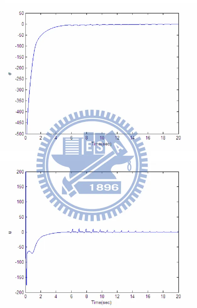
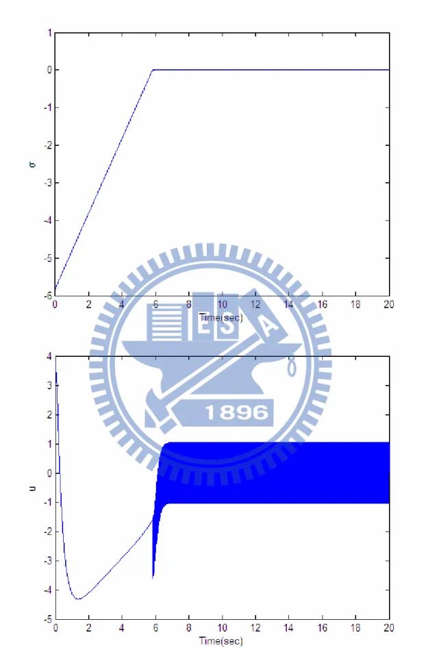
d = π − Figure 3.1 shows the time histories of the state, the

sliding variableσ , and the input (3.29) when x₁(0)=20o(

π

/9 rad), x₂(0)=

= ) 0 ( 3

x x₄(0)=0. Figure 3.2 shows the time histories of the state, the

sliding variable σ , and the input (3.29) when x1(0)=40o(2π/9 rad), x2(0)= =

) 0 ( 3

x x₄(0)=0. Figure 3.3 shows the time histories of the state, the

(37)

= ) 0 ( 3

x x₄(0)=0. In Figure 3.1, Figure 3.2, and Figure 3.3, it should be noted that

since it is impossible to switch the input u instantaneously, oscillations always occur in the sliding mode of a SMC system.It is observed that in our simulations the proposed controller (3.29) stabilizes the following two-rule fuzzy model (3.28).

(38)

(39)

(40)

30

(41)

(42)

(43)

(44)

(45)

(46)

36

Figure 3.3 Simulation results withx₁(0)=60o(π/3 rad), x₂(0)=x₃(0)=x₄(0)=0.

Example 3.2 Consider the following example of a ball and beam system [52], whose

dynamic equations are described as follows:

, 0 sin ₋ 2 ₌ +       ₊ _θ _θ_& && MG Mr r M R Jb

(

2 + +

)

θ +₂ θ + _cosθ =τ MGr r Mr J J

Mr _b && _&&

(3.30) where r is the ball position, θ is the beam angle, J is the moment of inertia of the

beam, M , J , and R are the mass, the moment of inertia, and the radius of the ball b

respectively, G is the acceleration of gravity, and τ is the torque applied to the

beam. Define /( / 2 ) M R J M

B= _b + and change the coordinates in the input space by using the

invertible transformation u J J Mr MGr r Mr cos b) 2 ₊ ₊ 2 ₊ ₊ = θ θ τ _& & (3.31)

線性矩陣不等式的強健適應滑差控制應用於T-S模糊系統

國立交通大學

電控工程研究所

博 士 論 文

線性矩陣不等式的強健適應滑差控制應用

於 T-S 模糊系統

Linear Matrix Inequality Based Adaptive Sliding

Control for Takagi-Sugeno Fuzzy Systems

研 究 生 ：劉松傑

指 導 教 授 ：林昇甫 博士

線性矩陣不等式的強健適應滑差控制應用於 T-S 模糊系統

Linear Matrix Inequality Based Adaptive Sliding Control for

Takagi-Sugeno Fuzzy Systems

研 究 生 ：劉松傑

Student: Sung-Chieh Liu

指 導 教 授 ：林昇甫 博士

Advisor: Dr. Sheng-Fuu Lin

國立交通大學

電控工程研究所

博士論文

線性矩陣不等式的強健適應滑差控制應用

於 T-S 模糊系統

國立交通大學 電控工程研究所

摘要

Linear Matrix Inequality Based Adaptive Sliding

Control for Takagi-Sugeno Fuzzy Systems

Institute of Electrical Control Engineering

National Chiao Tung University

ABSTRACT

誌謝

Contents

List of Figures

Symbol List

Chapter 1

Introduction

1.1 Motivation

1.2 Related Works

∫

∫ ∫

1.3 Approach

1.4 Organization of this Dissertation

Chapter 2

Foundations

2.1 Lyapunov Stability

{

}

∫

∫

2.2 Linear Matrix Inequality

∑

Chapter 3

LMI-Based Robust Sliding Control

3.1 Introduction

3.2 Robust Sliding Control for T-S Fuzzy Systems

3.2.1 System Formulation

[

]

∑

∑

∑

∑

∑

∑

[

]

[

]

[

]

∑

3.2.2 Sliding Control Design via LMI

[

]

∑

∑

∑

∑

∑

∑

∑

博士論文

研究生：劉松傑

指導教授：林昇甫博士

研究生：劉松傑

指導教授：林昇甫博士

國立交通大學電控工程研究所