相依截切資料的統計推論

國 立 交 通 大 學

統計學研究所

博士論文

相依截切資料的統計推論

Statistical Inference for

Dependent Truncation Data

Ph.D. Candidate: Takeshi Emura

Advisor: Dr. Weijing Wang

相依截切資料的統計推論

Statistical Inference for

Dependent Truncation Data

研 究 生：江村剛志 Student：Takeshi Emura

指導教授：王維菁 Advisor：Weijing Wang

國 立 交 通 大 學

統計學研究所

博 士 論 文

A Dissertation

Submitted to Institute of Statistics College of Science National Chiao Tung University

in partial Fulfillment of the Requirements for the Degree of Ph.D

in

Institute of Statistics June 2007

Hsinchu, Taiwan, Republic of China

Statistical Inference for

Dependent Truncation Data

Student：Takeshi Emura Advisor：Weijing Wang

Institute of Statistics

National Chiao Tung University

ABSTRACT

In this dissertation, we investigate the dependent relationship between two failure time variables which have a truncation relationship. Chaieb et al. (2006) considered semi-parametric framework under a “semi-survival” Archimedean-copula assumption and proposed estimating functions to estimate the association parameter, the truncation probability and the marginal functions.

In the first project, we adopt the same model assumption but propose different estimating methods. In particular we extend Clayton’s conditional likelihood approach (1978) to dependent truncation data for estimation of the association parameter. For marginal estimation, we propose a recursive algorithm and derive explicit formula to obtain the solution. The functional delta method is applied to establish large sample properties which can handle more general estimating functions than the U-statistic approach. Simulations are performed and the proposed methods are applied to the transfusion-related AIDS data for illustrative purposes.

Quasi-independence has been assumed by many inference methods for analyzing truncation data. By forming a series of 2× tables, we also propose a weighted log-rank 2 statisitcs for testing this assumption, which is our second project. Power improvement is possible by choosing an appropriate weight function. Here, we derive score tests when the dependence structure under the alternative hypothesis is specified semiparametrically. Asymptotic analysis and simulations are used to justify our proposed methods.

Table of Contents

Chapter 1 Introduction

1

1.1 Motivation and Background 1

1.2 Overview of the Proposal 4

Chapter 2 Literature Review

6

2.1 Association Measures and Copula Models 6

2.2 Semi-parametric Inference for Survival-copula Models 8

2.3 Association Measures and Copula Models Suitable for Truncation Data 9 2.4 Statistical Inference for Truncated Data under Quasi-Independence 11

2.5 Statistical Inference for Dependent Truncated Data 13

Chapter 3 The Proposed Approach for Semi-parametric Inference

16

3.1 Estimation of Association 16

3.1.1 Conditional Likelihood Approach 16

3.1.2 Estimation based on Two-by-two Tables 17

3.1.3 Construction based on concordance indicators 18

3.1.4 Equivalent condition for different approaches 19

3.2 Estimation of marginal functions and truncation probability 20

3.2.1 The approach of Chaieb et al. (2006) 20

3.2.2. Recursive Solution to the Moment Constraints 21

3.3 Asymptotic Analysis 23

3.3.1 General Results for Asymptotic Properties 23

3.3.2. Asymptotic Behavior under Independence 24

3.4 Extension and Modification 30

3.4.1 Extension under right censoring 30

3.4.2 Modification for small risk sets 32

3.5 Numerical analysis 33

3.5.1 Simulation studies 33

3.6. Conclusion 39

Appendices : Project 1

40

Appendix 3.A: Asymptotic Analysis 40

Appendix 3.B: Equivalence of Different Estimating Functions 47

Appendix 3.C: Examples of AC Models 48

Chapter

4

Testing

quasi-independence

51

4.1 The Proposed Test Statistics 52

4.1.1 Construction based on 2× table 2 52 4.1.2 Relationship with Tsai’s test 54

4.2 Conditional Score Test 55

4.2.1 Likelihood Construction 55

4.2.2 Semi-survival AC models 57

4.3 Asymptotic analysis 60

4.3.1 Asymptotic normality 60

4.3.2 Variance estimation: Empirical vs. Jackknife 62

4.4 Modification for Right Censoring 63

4.4.1 The Weighted Log-rank Statistics under Censoring 63

4.4.2 The Conditional Score test under Censoring 65

4.4.3 Asymptotic Analysis under Censoring 65

4.5 Numerical Studies 67

4.5.1 Comparing Two Variance Estimators 67

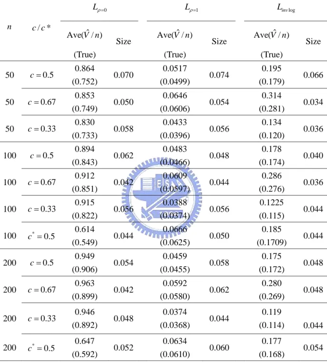
4.5.2 Size of the Weighted Log-rank Test 68

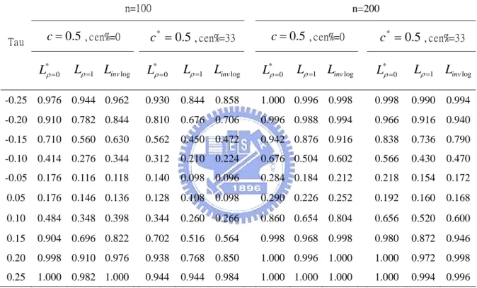
4.5.3 Power of the Tests 70

4.6 Data Analysis 76

4.7 Conclusion 77

Appendices : Project 2

79

Appendix 4.A: Asymptotic Analysis 79

Appendix 4.B: Proof of Rquivalence Formula 87

Chapter

5

Future

Work

90

Chapter 1 Introduction

1.1 Motivation and Background

In the thesis, we consider a pair of failure times (X,Y) which can be included in the sample only if X ≤ . The variable Y is said to be “left truncated” by X and X is said Y to be “right truncated” by Y . In many applications, usually one variable is of major interest while the other is nuisance. The book by Klein and Moeschberger (2003) mentioned an example which studied the survival distribution for elderly residents in a retirement center. In the example, X denotes a subject’s age of entering the retirement community and Y denotes the lifetime for the person. Notice that only those who had lived long enough to be eligible for joining the retirement community could be included in the sample. Therefore the truncation scheme has to be taken into account in the development of inference methods for Y . Most nonparametric inference methods for truncation data assume independence between X and Y (e.g. Lynden-Bell, 1971 and Woodroofe, 1985). Under this assumption, Lynden-Bell suggested to estimate Pr(Y > based on the product-limit expression of this t) quantity and thereafter many nice properties of the Kaplan-Meier estimator for right censored data have been extended to the truncation setting.

Unlike the situation of right censoring in which the independent censorship assumption is not testable, Tsai (1990) claimed that the independence assumption can be relaxed to a weaker assumption of “quasi-independence” and the latter can be verified nonparametrically. Tsai (1990) introduced a measure of “conditional Kendall’s tau” which was later applied to different truncation settings by Martin and Betensky (2005). Tsai also proposed a test of quasi-independence based on this measure. Alternatively, Chen, Tsai, and Chao (1996) suggested a conditional version of Pearson’s product-moment correlation coefficient, denoted as ρ_c, to measure the association between X and Y . Based on the sample version of ρ_c, they proposed a test for quasi-independence. However the method based on ρc can not be

extended to the more general situation that also includes right-censoring.

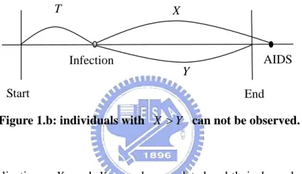
Figure 1.a: individuals with X ≤ can be observed. Y

Figure 1.b: individuals with X > can not be observed. Y

In some applications, X and Y may be correlated and their dependent relationship is of interest. Tsai (1990) applied his testing procedure to an example of transfusion-related AIDS study. Let T be the infection time of individuals, measured form the beginning of the study, and X be the incubation period from the time of infection to AIDS. Only individuals who developed AIDS by the end of study can be observed (see Figure 1.a). Since the total study period is 102 months, individuals with T + X ≤102 were included in the sample. Using the notation 102−T =Y , we view X as being right truncated by Y . Primary interest on this study focuses on the incubation distribution X . Dependence between X and Y might be of secondary interest. However applying Tsai’s method (1990), the assumption of quasi-independence was rejected. Positive association between X and Y means negative association between T and Y . That is the earlier the infection time, the larger the length of incubation. This surprising finding might shed some light on the study of

AIDS X T Y Start End Infection Start End X T Y AIDS Infection

population dynamics of AIDS.

Recently Chaieb et al. (2006) proposed a semi-parametric inference approach to assessing the dependence between X and Y under the assumption that the two variables jointly follow a modified version of an Archimedean copula (AC) model which adapts to the nature of truncation. Copula models have the nice feature that the dependence structure is modeled separately from the marginal effects. Semiparametric inference of copula models has received substantial attentions in the literature. There exist several ways of estimating the association parameter, for a specific copula model or a class of copula models, without specifying the marginal distributions. One popular approach, which has been taken by Oakes (1986) for right censored data and by Fine et al. (2000) for semi-competing risks data, is to utilize the concordance or discordance information for pairs of observations. This idea has been taken by Chaieb et al. (2006) in analysis of dependent truncation data. Compared with the previous results, the new challenge is that the association parameter can not be estimated without knowing the truncation probability. Hence the paper of Chaieb et al. (2006) also considered estimation of the truncation probability and the marginal functions. Their proposed algorithm can be considered as an extension of the method by Rivest and Wells (2001) who considered the situation of dependent censoring.

The dissertation contains two parts, both of which deal with possibly correlated truncation data. The first project was motivated by the paper of Chaieb et al. (2006) but a different inference approach is proposed. Besides proving a new method, we also aim to unify the two different types of inference approaches under a general framework. In the second project we study the problem of testing quasi-independence. Specifically we construct a testing procedure similar to the setup of the weighted Log-rank statistics constructed based on a series of two-by-two tables. The proposed test is nonparametric in the sense that no model assumption is needed. We also derive an equivalent expression of the proposed test statistics which allows us to compare different methods under the same framework. It turns out that the

proposed test statistic can be viewed as a generalized version of some existing tests including Tsai’s test (1990). Furthermore, in both projects, the likelihood information is utilized to improve efficiency of the proposed estimator or power of the proposed test.

1.2 Overview of the Dissertation

Literature review is given in Chapter 2. The first part focuses on bivariate analysis in which some common association measures and models for lifetime variables are introduced and related inference results are reviewed. In particular the family of copula models and its sub-class, Archimedean copula models, are discussed. Different semi-parametric inference approaches developed for analyzing data which follow copula models are examined. Specifically we focus on three methods of constructing an estimating function of the copula association parameter. One is the conditional likelihood approach which first appeared in the landmark paper of Clayton (1978) for bivariate censored data. The second approach utilizes concordant information of paired observations and has been applied to bivariate censored data by Oakes (1986), Fine (2001) for semi-competing risks data and Chaieb et al. (2006) for dependent truncation data. The third approach suggests to construct estimating functions based on a series of two-by-two tables which has been applied by Day et al. (1997) and Wang (2003) in analysis of semi-competing risks data. In the second part of Chapter 2, we review the literature on marginal estimation. The idea of product-limit expression has been used to construct the Kaplan-Meier estimator and the Lynden-Bell’s estimator under independent censoring and (quasi-) independent truncation respectively. Many papers have studied the situation when the assumption of independence fails. We will review the papers which use copula models to specify the dependence relationship.

Chapters 3 and 4 contain our results for the two projects. Specifically, in Chapter 3, we consider semi-parametric inference based on semi-survival AC models under the framework

proposed by Chaieb et al. (2006). Besides proposing a new inference approach which turns out to be more efficient, we also establish the relationships among different estimating functions. The unified framework allows us to compare different methods in a systematic way and hopefully such analysis can facilitate future development of statistical methodology or inference theory. In Chapter 4, we consider the problem of testing quasi-independence for truncation data. We propose a general class of test statistics which include some existing tests as special cases. In addition, we discuss how to incorporate additional likelihood information provided by the alternative hypothesis to improve the power of the test.

Chapter 2 Literature Review

2.1 Association Measures and Copula Models

To simplify the analysis, let (X,Y) be a pair of continuous failure time variables. Kendall’s tau, denoted as τ , is a rank-correlation measure which is often used to describe the level of global association between X and Y . Let (Xi,Yi) and (Xj,Yj) be two

independent replications of (X,Y) and Δij =I{(Xi −Xj)(Yi −Yj)>0} indicates whether the two pairs are concordant (Δij =1) or discordant (Δij =0). Kendall’s tau is defined as

1 ) ( 2 ) 0 Pr( ) 1 Pr( ) 0 ) )( Pr(( ) 0 ) )( Pr(( − Δ = = Δ − = Δ = < − − − > − − = ij ij ij j i j i j i j i E Y Y X X Y Y X X τ (2.1)

We note that τ has the nice property of rank invariance since its value is unchanged by both linear or nonlinear increasing transformations. For measuring local dependence or time-varying association, Oakes (1989) proposed the following cross ratio-function:

y y Y x X x y Y x X y Y x X y x y Y x X y x ∂ > > ∂ ⋅ ∂ > > ∂ > > ⋅ ∂ ∂ > > ∂ = / ) , Pr( / ) , Pr( ) , Pr( / ) , Pr( ) , ( ~ 2 θ . (2.2)

Note that θ~(x,y) =1 implies independence at time (x,y), 1θ~(x,y)> implies positive association and θ~(x,y)<1 implies negative association respectively. Oakes also derived another useful expression of θ~(x,y) as the odds ratio of concordance for the ( ji, ) pairs given that (X~_ij,Y~_ij)=(x,y). It follows that

) , ( ~ y x θ ) ~ , ~ | 0 Pr( ) ~ , ~ | 1 Pr( y Y x X y Y x X ij ij ij ij ij ij = = = Δ = = = Δ = . (2.3)

The two expressions in (2.2) and (2.3) are useful in the development of inference methods for copula models which be introduced later.

Copulas form a class of bivariate distribution functions whose marginals are uniform on the unit interval (Genest and MacKay, 1986). In applications of lifetime data analysis, the copula structure is usually imposed on the joint survival function such that one can write

)} Pr( ), {Pr( ) , Pr(X > xY > y =C X > x Y > y ,

where the function C(u,v):[0,1]2 →[0,1] can be viewed as the survival copula of )

,

(X Y (Nelsen, 1999, p.28). When the copula function is parameterized as C_α( vu, ), the parameter α is related to Kendall’s tau such that

τ 4 ( , ) ( , ) 1 1 0 1 0 − =

∫∫

C_α u v C_α du dv .

The copula family has the nice feature that the dependence structure can be studied separately from the marginal distributions. In practical applications, the association parameter α is often the major of interest and can be estimated without specifying the marginal distributions. We will review existing semi-parametric inference methods developed for copula models later.

Archimedean copulas (AC) are special copula models which possess useful analytical properties. For an AC model, the bivariate copula function C_α( vu, ) can be further simplified as )} ( ) ( { ) , (u v 1 u v C_α =φ_α− φ_α +φ_α for u,v∈[0,1], (2.4) where ]φ_α(.):[0,1]→[0,∞ is a univariate function which have two continuous derivatives satisfying φ_α(1)=0,φ_α′(t)=∂φ_α(t)/∂t<0and φ_α′′(t)=∂2φ_α(t)/∂t2 >0. A special property of AC models is that the bivariate relationship can be summarized by the univatiate function

(.)

α

φ . In applications, selecting an appropriate Archimedean copula model refers to identifying the form of φ_α(.). For an AC model indexed by φ_α(⋅), Oakes (1989) showed that

)} , {Pr( ) , ( * y Y x X y x =θ_α > >

) ( / ) ( ) (v v _α v _α v α φ φ θ =− ⋅ ′′ ′ . (2.5)

When )φ_α(t)=−log(t , X and Y are independent. For the Clayton model with

1 )

( = −(α−1) −

α

φ t t (α >1) , it can be shown that θ_α(v)=α.

2.2 Semi-parametric Inference for Survival-copula Models

There have been substantial interests in developing inference methods for estimating the association parameter of a copula model without specifying the marginal distributions. Most results have been derived for survival copula models in which the copula structure is imposed on the joint survival function as mentioned earlier. Early work focused on the Clayton model (Clayton, 1978), a member of the AC family with φα(t)=t−(α−1) −1 (α >1) and

α

θ~(x,y)= . Clayton (1978) proposed to maximize a product of conditional probabilities and later his estimator was re-expressed by Clayton and Cuzick (1985) as a weighted form of Oakes’ concordance estimator (Oakes, 1982). The new representation is related to a U-statistics which turns out to be useful in the establishment of asymptotic properties (Oakes, 1986).

There has been a trend to develop unified inference approaches suitable for a class of copula models rather than a single member, say the Clayton model. The approach of two-stage estimation has been adopted by Genest et al. (1995), Shih and Louis (1995) and Wang and Ding (2000) for complete data, bivariate right censored data and current status data respectively. Specifically C_α( vu, ) can be viewed as the joint survival function of

) ( X

S

U = X and V =SY(Y) , where SX(t)=Pr(X >t) and SY(t)=Pr(Y >t) . If the

marginals were completely specified, then a random sample of (U,V) , denoted as )) ( ), ( ( ) ,

(Ui Vi = SX Xi SY Yi (i=1,...,n) , or its censored version can be obtained in

sample of (U,V) is not available. These papers suggested a two-stage estimation procedure. In the first stage, the marginal distributions are estimated by applying existing nonparametric methods. In the second stage, the marginal estimators are treated as “pseudo observations” in the likelihood constructed based on C_α( vu, ) . Despite of its simplicity, this approach becomes infeasible when the data involve dependent censoring or other complicated situations so that the marginal distributions become non-identifiable nonparametrically.

Semi-competing risks data provides such an example in which one variable is a competing risk for the other but not vise versa and hence the aforementioned two-stage estimation procedure is not applicable. For semi-competing risks data., two different approaches have been adopted. Specifically Day et al. (1997) and Wang (2003) constructed estimating functions, in the form of the log-rank statistics, based on a series of two-by-two tables in which the odds ratio of the table reveals the information of association. Day et al. (1997) considered the Clayton model with θ~(x,y)=α and Wang (2003) extended the idea to the whole AC family using the properties of (2.5). The second approach was proposed by Fine et al. (2001) who utilized equation (2.3) to construct an estimating function for the Clayton model based on the concordance indicator Δ whose expected value contains the ij

information of α .

2.3 Association Measures and Copula Models Suitable for Truncation Data

For truncation data, we observe (X,Y) only if X ≤ . Hence joint analysis has to be Y restricted in the upper wedge R_U ={(x,y):0≤ x≤ y<∞}. Consequently the aforementioned descriptive measures and models may not be directly applicable to describe (X,Y) if they have a truncation relationship.

suggested to consider the event A_ij ={ω:X_ij(ω)≤Y~_ij(ω)} , where X_ij = X_i ∨X_j ,

j i ij Y Y

Y~ = ∧ . Notice that under the truncation scheme, as long as (X_ij,Y~_ij)∈R_U , or equivalently X_ij ≤Y~_ij , it follows that (X_i,Y_i) and (X_j,Y_j) are both in R . By _U conditioning on the event A , Tsai proposed the modified version of Kendall’s tau such that _ij

1 ) | ( 2 Δ − = _{ij ij} a E A τ , (2.6)

where )(X_i,Y_i and (X_j,Y_j) be two independent replications of (X,Y), which are known to satisfy the truncation scheme with X_i ≤ and Y_i X_j ≤ given Y_j A . The measure _ij τ_a is a well-defined measure for truncation data.

To measure local dependence for truncation data, Chaieb et al. (2006) adopted Tsai’s idea to modify equation (2.3). Specifically for x≤ they proposed to consider y

)) (x, ) ~ , ( | 1 Pr( )) (x, ) ~ , ( | 0 Pr( ) , ( * y Y X y Y X y x ij ij ij ij ij ij = = Δ = = Δ = θ (2.7)

The value of θ*(x,y) can be interpreted in the same way as θ~(x,y). Notice that θ*(x,y) in (2.7) and θ~(x,y) in (2.3) differ in the way of choosing the corner position. Specifically for θ~(x,y), the corner is chosen to be (X~_ij,Y~_ij)=(X_i ∧X_j,Y_i ∧Y_j) while, for truncation data, the corner is (X_ij,Y~_ij)=(X_i ∧X_j,Y_i ∨Y_j). The measure θ~(x,y) is not appropriate for truncation data since given ) U

~ ,

(Xij Yij ∈R , it is still possible that (Xi,Yi) or (Xj,Yj) may

fall outside R . In contrast, by choosing _U (Xij,Y~ij) as the target in making the conditioning

arguments, the two points will fall in R ._U

For truncation data, Chaieb et al. (2006) suggested to impose the model structure on the “semi-survival” function, defined as Pr(X≤x,Y>y) (x≤ ), which is a more natural y

descriptive measure than the joint survival function Pr(X>x,Y>y). Furthermore since no information is available in the lower wedge {(x,y):0≤ y< x<∞} , the function

) | , ( Pr ) , (x y = X≤xY>y X≤Y

π can be identifiable nonparametrically while Pr(X≤x,Y>y)

is not. Accordingly, adapting to the nature of truncation, Chaieb et al. (2006) suggested to impose the AC structure on π(x,y) such that

c y S x F y x, ) [ { _X( )} { _Y( )}]/ (

φ

_α 1

φ

_α

φ

_α

π

= − + (x≤ ), y (2.8) where F_X(⋅) and S_Y(⋅) are continuous distribution and survival functions respectively and

c is a unknown normalizing constant satisfying

∫∫

< − ₊ ∂ ∂ ∂ − = y x Y X x S y dxdy F y x c 1[ { ( )} { ( )}] 2 α α α φ φ φ . (2.9)

Note that under model (2.8), the normalizing constant c may not be the truncation proportion Pr(X ≤Y), but it makes the model (2.8) to have a valid density function. Note that when φ_α(t)=−log(t), quasi-independence between X and Y holds.

2.4 Statistical Inference for Truncated Data under Quasi-Independence

For truncation data, we observe (X,Y) only if X ≤ . Replications of Y (X,Y) are located in the upper wedge RU ={(x,y):0≤x≤ y<∞} . The sample consists of

)} , , 1 ( ) , (

{ X_j Y_j j = … n subject to X_j ≤Y_j . We can consider the sample )} , , 1 ( ) , (

{ X_j Y_j j = … n as iid from the cumulative distribution function ) | , Pr( ) , (x y X x Y y X Y

H = ≤ ≤ ≤ . Let X and Y be positive independent random variables having the marginal distribution functions Pr(X ≤ x) and Pr(Y ≤ y) . The independence between X and Y cannot be tested from data since the information for the lower wedge is unavailable. Thus, the independence assumption

∫∫

∫∫

≤ ≤ ≤ ≤ ≤ ≤ ≤ = v u x y v Y d u X d v u I v Y d u X d v u I y x H( , ) ( ) Pr( ) Pr( ) ( ) Pr( ) Pr( ) 0 0

may not be acceptable unless independence between X and Y is known from prior knowledge. Instead, Wang, Jewell and Tsai (1986) assumed the model,

0 H : H x y I u v dF_X u dF_Y v c x y / ) ( ) ( ) ( ) , ( 0 0

∫∫

≤ = ,

where FX andFY are arbitrary distribution functions and c is the normalizing constant

satisfying

∫∫

≤ = y x Y X x dF y dF c₀ ( ) ( ).

Tsai (1990) called the assumption under H as “quasi-independence”. 0

Using the semi-survival function, the assumption of quasi-independence can be simplified as

0

H : Pr(X ≤ x,Y > y|X ≤Y)=F_X(x)S_Y(y)/c,

where FX and SY are arbitrary right continuous distribution and survival functions, and c 0

is the normalizing constant satisfying

∫∫

≤ − = y x Y X x dS y dF c₀ ( ) ( ).

Define the support of X as [xL,xU] , where xL =inf{u;FX(u)>0} and

} 1 ) ( ; sup{ < = u F u

x_{U X} . Similarly define the support of Y as [y_L,y_U] , where

} 1 ) ( ; inf{ < = u S u

yL Y and yU =sup{u;SY(u)>0}. It is usually assumed that xL ≤ yU so

that c>0 . In general, the true distributions F_X and S_Y cannot be estimated nonparametrically without further assumptions. However the following conditional distributions are estimable:

) , | Pr( ) ( 0 L U X x X x X y Y x F = ≤ ≤ ≥ , )S_Y0(y)=Pr(Y > y|X ≤ y_U,Y ≥ x_L .

Under the assumption of quasi-independence, Lynden-Bell (1971) derived the nonparametric maximum likelihood estimators (NPMLE) for the two marginal distributions which can be

expressed as following explicit formula:

∏

> ⎭⎬ ⎫ ⎩ ⎨ ⎧ ₋ − − = x u X u u R u R u R x F ) , ( ) 0 , ( ) 0 , ( 1 ) ( ˆ _,

∏

≤ ⎭⎬ ⎫ ⎩ ⎨ ⎧ ₋ ∞ − ∞ + = y u Y u u R u R u R y S ) , ( ) , ( ) , ( 1 ) ( ˆ _{, (2.10)} where R(x,y)

∑

= ≥ ≤ = n j j j x Y y X I 1 ) ,

( . Woodroofe (1985) showed the uniform consistency results 0 | ) ( ) ( ˆ | sup_x>0 F_X x −F_X0 x ⎯⎯→P ; 0sup_y>0 |Sˆ_Y(y)−S_Y0(y)|⎯⎯→P .

Wang et al. (1986) derived a simple asymptotic variance for the Lynden-Bell’s estimator, which turns out to be an analogy of the asymptotic variance of the Kaplan-Meier estimator. A necessary condition for the above Lynden-Bell’s estimators to be consistent estimators for

X

F and S_Y is that x_U < y_U and x_L < y_L so that F_X =F_X0 and S_Y =S_Y0. In other words, there exists two positive number y_L < x_U such that

0 ) ( L > X y

F , SY(yL)=1, 1FX(xU)= and SY(xU)>0.

2.5 Statistical Inference for Dependent Truncation Data

Recall the modified version of Kendall’s tau proposed by Tsai in (2.6): 1 ) | ( 2 Δ − = ij ij a E A τ .

Based on the sample consists of {(X_j,Y_j)(j=1,…,n)} subject to X_j ≤ , Tsai (1990) Y_j proposed to estimate τ_a by 1 } { } { 2 } { } { )} )( sgn{( ˆ − ⋅ Δ ⋅ = − − =

∑

∑

∑

∑

< < < < j i ij j i ij ij j i ij j i ij j i j i a A I A I A I A I Y Y X X τ . (2.11)

Under the semi-survival AC assumption in (2.8), Chaieb et al. (2006) proposed to estimate

α

by utilizing the concordant information provided by Δ since its (conditional) _ij expected value reveals the information of α . Their idea can be viewed as an extension of the

methods by Clayton and Cuzick (1985) for bivariate right censored data and by Fine et al. (2001) for semi-competing risks data. Specifically under the semi-survival AC model assumption, it follows that

)} , ( { 1 1 ) ) , ( ) ~ , ( | ( y x c A y x Y X E ij ij ij ij _{θ π} α + = ∈ = Δ ,

where the relationship between θα(.) and φα (.) is given in equation (2.5). Accordingly

they proposed the following estimating function:

∑

< ⎥ ⎥ ⎦ ⎤ ⎢ ⎢ ⎣ ⎡ + − Δ = j i ij ij ij ij ij c ij w Y X c Y X w A c U )} ~ , ( ˆ { 1 1 ) ~ , ( ~ } { 1 ) , ( ~ , _{θ π} α α α , (2.12)

where )w~_α,c(x,y is a weight function and

) , ( ˆ x y π

∑

= > ≤ = n i i i x Y y n X I 1 / ) , ( .

Note that when w~α,c(x, y) =1, the above estimating function is equivalent to

∑

∑

< < + − = j i ij j i ij ij ij ij ij a A I A I Y X c Y X c } { } { )}] ~ , ( ˆ { 1 /[ )}] ~ , ( ˆ { 1 [ ˆ π θ π θ τ α α , (2.13)

where the right-hand side can be viewed as an model-based estimator of τ_a.

Notice that U~_w(α,c) involves the truncation proportion parameter c which is unknown. In the special case of the Clayton model with φα(t)=t−(α−1) −1 (α >1) and

α

θ_α(v)= , U~_w(α,c) depends only on α . This implies that U~w(α,c) alone is not enough

for estimation of α . Chaiebl et al. (2006) proposed their second estimating procedure which was motivated by the paper of Rivest and Wells (2001) on marginal estimation for dependent censored data. Their idea was inspired by the paper of Zheng and Klein (1995).

Now we describe the second estimation procedure proposed by Chaiebl et al. (2006). Let

n

t

∑

≤ ≥ = j j j t Y t X I t t

R(, ) ( , ) . Replacing π(t,t) by R(t,t+)/n in equation (2.8) , they obtained a set of estimating equations:

)} ( { )} ( { ) , ( i Y i X i i t S t F n t t R c _{α α} α φ φ φ = + ⎭ ⎬ ⎫ ⎩ ⎨ ⎧ + (i=1,…,2n−1). (2.14) To solve the above equations, Chaieb et al. (2006) modified the algorithm of Rivest and Wells (2001) originally proposed for dependent censored data. Specifically they first estimated the jumps, φ_α{S_Y(t_i)}−φ_α{S_Y(t_i−)} and φ_α{F_X(t_i)}−φ_α{F_X(t_i+)}, and then summed them up over all the failure times prior to t to obtain the estimators for φ_α{F_X(t)} and

)} ( {SY t

α

φ . Then by plugging in all the marginal estimators into the equations in (2.14), an estimating function for c can be obtained. In Section 3 and Section 4, we propose different methods for estimating (α,c) and solving the equations in (2.14), respectively.

Chapter 3 The Proposed Approach for

Semi-parametric Inference

In this chapter, we develop a new inference approach to analyzing semi-survival AC models of the form in (2-8). Specifically two types of estimating functions are needed to estimate the unknown parameters, α, c, FX(⋅) and SY(⋅) . One is for estimating the

association parameter and the other is related to marginal estimation. The present method is semiparametric in the sense that we do not specify the form of FX(⋅) and SY(⋅), but specify

the functional form φ_α(.).

3.1 Estimation of Association

3.1.1. Conditional Likelihood Approach

In this section, we consider estimation of α under the semi-survival AC model in (2.8). To simplify the analysis, we assume that there is no ties and, temporarily, we ignore external censoring. The sample consists of {(X_j,Y_j)(j =1,…,n)} subject to X_j ≤Y_j. Here we generalize Clayton’s likelihood approach (Clayton, 1978) to truncation data. Define the set of grid points as follows:

⎭ ⎬ ⎫ ⎩ ⎨ ⎧ = ≥ = = = ≤ ≤ =

∑

∑

= = 1 ) , ( , 1 ) , ( , | ) , ( 1 1 n j j j n j j j x Y y I X x Y y X I y x y x ϕ .

For a point (x,y) in ϕ, we can define the “risk set” ℜ(x,y)={i;X_i ≤x,Y_i ≥ y}. Denote ) , (x y R

∑

= ≥ ≤ = n i j j x Y y X I 1 ) ,

( as the number of observations in ℜ(x,y) . Let

∑

= = = = Δ n i j j xY y X I y x 1 ) , ( ) ,

( , which indicates whether failure occurs at (x,y). Given r

y x

R( , )= for (x,y)∈ϕ and under model (2.8), the variable Δ(x,y) follows a Bernoulli distribution with the probability

)} , ( { 1 )} , ( { } ) , ( , ) , ( | 1 ) , ( Pr{ y x c r y x c y x r y x R y x π θ π θ ϕ α α + − = ∈ = = Δ , (3.1)

where the relationship between θ_α(.) and φ_α(.) is stated in equation (2.5). Ignoring the marginal distribution Pr(R(x,y)=r|(x,y)∈ϕ} which may contain only little information about α , we can construct the following conditional likelihood function

∏

∈ Δ − Δ ⎥ ⎦ ⎤ ⎢ ⎣ ⎡ + − − ⎥ ⎦ ⎤ ⎢ ⎣ ⎡ + − = ϕ α α α π θ π θ π θ π α ) , ( ) , ( 1 ) , ( )} , ( { 1 1 )} , ( { 1 )} , ( { ) ), , ( , ( y x y x y x y x c r r y x c r y x c c y x L .

The nuisance parameter π(x,y) can be estimated nonparametrically by πˆ(x,y)=R(x,y)/n. Differentiating logL(α,πˆ(x,y),c) with respect to α , we get the following estimating function

∫∫

∈ ⎥ ⎦ ⎤ ⎢ ⎣ ⎡ + − − Δ = ϕ α α α α π θ π θ π θ π θ α ) , ( ( , ) 1 { ˆ( , )} )} , ( ˆ { ) , ( )} , ( ˆ { )} , ( ˆ { ) , ( y x L y x c y x R y x c y x y x c y x c c U , (3.2) where θ_α(v)=∂θ_α(v)/∂α .

For the Clayton model with φα(t)=t−(α−1) −1 (α >1) and θα(v)=α , UL(α,c)

depends only on α . The proposed estimator of α can be obtained by solving

0 1 ) , ( ) , ( 1 ) ( ) , ( = ⎥ ⎦ ⎤ ⎢ ⎣ ⎡ + − − Δ =

∫∫

∈ϕ α α α α y x L y x R y x U .

However for other members in the AC family, estimation of α requires the information of

c. It is important to note that, for most models, ∂logL(α,c)/∂c yields the same estimating function as U_L(α,c). This implies that the likelihood function can not identify (α,c) simultaneously. Joint estimation of (α,c)will be discussed later in Section 3.2.

3.1.2 Estimation based on Two-by-Two Tables

Following the ideas proposed by Day et al. (1997) and Wang (2003), we can construct the following 2× table at an observed failure point 2 (x,y) with x≤ y . Let

∑

= • = ≤ = n i i i x Y y X I dy x N 1 1( , ) ( , ) and

∑

= • = = ≥ n i i i x Y y X I dy x N 1

1 ( , ) ( , ) . The table can be

represented as follows:

Table: Two-by-two Table for Truncated Data

The odds ratio of the above table is the sample analogy of the cross ratio function ) , ( * y x

θ defined in (2.7). Given the marginal counts, the conditional mean of Δ(x,y) can be derived as a function of θ*(x,y) or θ_α{cπ(x,y)} under model (2.8). The nuisance parameter

π

(x,y) can be estimated by πˆ(x,y). Motivated by the log-rank type statistic, we can combine all the tables at different values of (x,y) and then construct the following estimating function

∫∫

≤ • • ⎥ ⎦ ⎤ ⎢ ⎣ ⎡ + − − Δ = y x c w y x c y x R y x c dy x N y dx N y x y x w c U )} , ( ˆ { 1 ) , ( )} , ( ˆ { ) , ( ) , ( ) , ( ) , ( ) , ( 1 1 , _{θ π} π θ α α α α

∫∫

∈ ⎥⎦ ⎤ ⎢ ⎣ ⎡ + − − Δ = ϕ α α α _{θ π} π θ ) , ( , )} , ( ˆ { 1 ) , ( )} , ( ˆ { ) , ( ) , ( y x c y x c y x R y x c y x y x w , (3.3)

where w_α,c(x,y) is a weight function. Note that in derivation of (3.3), we use the assumption that the data have no ties and hence N_1•(dx,y)N_•1(x,dy)=1 if and only if

ϕ ∈ ) ,

(x y .

3.1.3 Construction based on Concordance Indicators

Here we review the idea proposed by Chaieb et al. (2006) and present a more general version of their estimating function . Based on (2.7) and for x≤ , it follows that y

y Y = Y > y x X = Δ(x,y) N1•(dx,y) x X < ) , ( 1 x dy N_• R(x,y)

)} ~ , ( { 1 1 ) ), ~ , ( | ( ij ij ij ij ij ij Y X c A Y X E π θ_α + = Δ (3.4)

Recall that if the event A_ij ={X_ij ≤Y~_ij} happens, the two pairs (X_i,Y_i) and (X_j,Y_j) will be located in the identifiable region R for certain. The following function can be viewed as U

a generalization of Oakes’ method (1986):

∑

< ⎥⎥⎦ ⎤ ⎢ ⎢ ⎣ ⎡ + − Δ = j i ij ij ij ij ij c ij w Y X c Y X w A c U )} ~ , ( ˆ { 1 1 ) ~ , ( ~ } { 1 ) , ( ~ , θ π α α α (3.5)

where )w~α_,c(x,y is a weight function. Note that the estimating function proposed by Chaieb et al. (2006) sets w~α,c(x, y) =1, and is related to the conditional Kendall’s tau as mentioned

in equation (2.13).

3.1.4 Equivalence Condition for Different Approaches

Now we establish the relationship among different estimating functions. This idea was motivated by the analysis of Clayton & Cuzick (1985) who expressed Clayton’s likelihood estimator in terms of concordance/discordance indicators. Consider the truncation setting. Some algebraic calculations yield the following identity:

∫∫

∈ ⎥ ⎦ ⎤ ⎢ ⎣ ⎡ + − − Δ ϕ α α α _{θ π} π θ ) , ( , )} , ( ˆ { 1 ) , ( )} , ( ˆ { ) , ( ) , ( y x c y x c y x R y x c y x y x w

∑

< ⎥ ⎥ ⎦ ⎤ ⎢ ⎢ ⎣ ⎡ + − Δ + − + − = j i _{ij ij} ij ij ij ij ij ij ij ij ij c ij Y X c Y X c Y X R Y X c Y X w A )} ~ , ( ˆ { 1 1 )} ~ , ( ˆ { 1 ) ~ , ( )}] ~ , ( ˆ { 1 )[ ~ , ( } { 1 , π θ π θ π θ α α α α . (3.6)

The above equation provides a unified framework for comparing different estimating functions. Our proposed estimating function U_L(α,c) using the conditional likelihood principle, is a special case of Uw(α,c) constructed based on the two-by-two construction with the weight function:

)} , ( ˆ { / )} , ( ˆ { ) , ( , x y c x y c x y w_αc =θ_α π θ_α π .

Furthermore UL(α,c) is also a special case of ( , ) ~

c

U_w α , constructed based on the concordance indicators, with the weight function:

)} , ( ˆ { 1 ) , ( )} , ( ˆ { 1 )} , ( ˆ { )} , ( ˆ { ) , ( ~ , y x c y x R y x c y x c y x c y x w _c π θ π θ π θ π θ α α α α α _{− +} + − = . (3.7)

The estimator proposed by Chaieb et al. (2006) is Uw(α,c) with

)} , ( ˆ { 1 )} , ( ˆ { 1 ) , ( ) , ( , y x c y x c y x R y x w _c π θ π θ α α α ₊ + − − = .

Its another representation is of the form U~w(α,c) with w~α,c(x, y) =1.

The above analysis implies that the three different estimation procedures yield the same form of estimating functions with different choices of the weight function. Now the next question is which weight function produces better results? Some authors such as Fine et al. (2001) have suggested practical guidelines for choosing the weight function under Clayton model but did not provide any theoretical justification. It seems that no simple theory is available for choosing the optimal weight in the estimating function (3-5). Here we recommend to use UL(α,c) since it utilizes some likelihood information. We will see in our

simulations that it also produces more efficient results than the weighted concordance estimator with w~α,c(x, y) =1.

3.2 Estimation of Marginal Functions and Truncation Probability

3.2.1 The Approach of Chaieb et al. (2006)

Here we adopt the framework of Chaiebl et al. (2006) but propose a different estimating algorithm. Let’s briefly describe their setup. Let t1 < <t2n be ordered observed points of

) , , , , , (X₁ … X_n Y₁ …Y_n and t₀ =0. Replacing π( tt, )by R t t n I X t Y t n j j j , )/ ( / ) , ( + ≡

∑

≤ >

)} ( { )} ( { ) , ( i Y i X i i t S t F n t t R c _{α α} α φ φ φ = + ⎭ ⎬ ⎫ ⎩ ⎨ ⎧ + (i=1,…,2n−1). (3.8) The idea of constructing the above estimating equations was motivated by the paper of Rivest and Wells (2001) who considered dependent censoring. For solving the equations, Chaieb et al. (2006) mimicked the approach of Rivest and Wells (2001) by estimating the difference

)} ( { )} ( {S_Y t_i − _α S_Y t_i− α φ

φ and φ_α{F_X(t_i)}−φ_α{F_X(t_i+)}. Then the estimated differences

are summed up to obtain the estimators of (φ_α{F_X(t_j)},φ_α{S_Y(t_j)}). The marginal estimators are plugged into equation (3-8) to obtain an estimating function involving (α,c). We find that it is difficult to understand the algorithm of Chaieb et al. (2006) and hence decide to propose a different algorithm.

3.2.2 Recursive Solution to the Moment Constraints

Here we propose to solve the equations in (3-8) in a different way. Suppose that Fˆ and _X

Y

Sˆ are step functions with jumps only at observed points. Then, the unknown parameters are

2 2 1 1), , ( ), ( ), , ( )} ( , , {α c F_X X … F_X X_n S_Y Y − … S_Y Y_n− ∈R n+ .

Total 2n+2 non-homogeneous moment constraints are needed to produce a unique solution to the set of equations. However (3.8) only contains 2n−1equations which permit numerous solutions. With no prior information at hand, two boundary conditions Fˆ_X(t_2n−1)=1 and

1 ) ( ˆ 1 = t

S_Y would provide reasonable candidates for the additional constraints to be added into (3.8). Together with the constraint UL(α,c)=0 of the likelihood equation, we obtain the full

2

2n+ equations, giving a unique moment estimator for

)} ( , ), ( ), ( , ), ( , , {α c FX X1 … FX Xn SY Y1− … SY Yn− .

Fixing an arbitrary value for (α,c), we regard an equation in (3.8) as an estimating function for {FX(ti),SY(ti)}. For instance, the initial constraint SˆY(t1)=1 immediately gives

the solution (Fˆ_X(t₁)=cR(t₁,t₁+)/n,Sˆ_Y(t_j)=1). The proposed procedure can be performed successively for j=1,…,2n−1.

(Step 1) If t corresponds to an observed value of X , set _j

)} ( ˆ { )} ( ˆ {SY tj = α SY tj−1 α φ φ and {ˆ ( )} ( , ) {ˆY( j)} j j j X S t n t t R c t F _{α α} α φ φ φ − ⎭ ⎬ ⎫ ⎩ ⎨ ⎧ + = ;

and if t corresponds to an observed value of Y , set _j

)} ( ˆ { )} ( ˆ {FX tj = α FX tj−1 α φ φ and {ˆ ( )} ( , ) {ˆX( j)} j j j Y F t n t t R c t S _{α α} α φ φ φ − ⎭ ⎬ ⎫ ⎩ ⎨ ⎧ + = .

(Step 2) Set U_c(α,c)=φ_α{Fˆ_X(x_(n))}= 0 to meet the assumption FˆX(t2n−1)=1. Jointly

solving this equation and U_L(α,c)=0 gives the estimators of (α,c), denoted as (αˆ,cˆ).

(Step 3) Redo (Step 1) by setting (α,c)=(αˆ,cˆ) obtained in (Step 2) and then update )}) ( ˆ { )}, ( ˆ { (φ_α F_X t_j φ_α S_Y t_j .

We can show that the solutions to the above algorithm have the following explicit formula:

⎟ ⎠ ⎞ ⎜ ⎝ ⎛ + ⎥ ⎥ ⎦ ⎤ ⎢ ⎢ ⎣ ⎡ ⎪⎭ ⎪ ⎬ ⎫ ⎪⎩ ⎪ ⎨ ⎧ − − ⎪⎭ ⎪ ⎬ ⎫ ⎪⎩ ⎪ ⎨ ⎧ =

∑

≤ < n c n x R c n x R c t F t x x j j j X j α α α α φ φ φ φ ) 1 ( ; 1 ) ( ~ ) ( ~ )} ( ˆ { , (3.9)

∑

≤ ⎥ ⎥ ⎦ ⎤ ⎢ ⎢ ⎣ ⎡ ⎪⎭ ⎪ ⎬ ⎫ ⎪⎩ ⎪ ⎨ ⎧ − − ⎪⎭ ⎪ ⎬ ⎫ ⎪⎩ ⎪ ⎨ ⎧ − = t y j j j Y j n y R c n y R c t S ; 1 ) ( ~ ) ( ~ )} ( ˆ { _{α α} α φ φ φ , (3.10) where )R~(t)=R(t,t , min( ) ,..., 1 ) 1 ( i n i X x = = and min( ) ,..., 1 ) 1 ( i n i Y y = = , and ⎟ ⎠ ⎞ ⎜ ⎝ ⎛ + ⎥ ⎥ ⎦ ⎤ ⎢ ⎢ ⎣ ⎡ ⎪⎭ ⎪ ⎬ ⎫ ⎪⎩ ⎪ ⎨ ⎧ − − ⎪⎭ ⎪ ⎬ ⎫ ⎪⎩ ⎪ ⎨ ⎧ =

∑

< n c n x R c n x R c c U j x x j j j c α φα φα φα ) 1 ( ; 1 ) ( ~ ) ( ~ ) , ( , (3.11)

In the case of quasi-independence with φ_α(t)=−log(t), equations (3.9) , (3.10) and (3.11) reduce to the Lynden-Bell’s estimators and the natural estimator of the truncation proportion (He and Yang, 1998). It is worthy to note that the representation of the

Lynden-Bell’s estimator as a solution to the moment equation in (3.8) with φ_α(t)=−log(t) is new in the literature. Compared with the traditional expression as a product-limit estimator, our approach provides a more general estimating scheme which allows for dependent truncation.

In principle, any other boundary constraints imposed on F_X(t_2n−1) and SY(t1) can give

a different but unique solution to (3.8) and U_L(α,c)=0. Here, our subjective choice of using 1 ) ( ˆ 1 2n− = X t

F and SˆY(t1)=1 facilitates the proposed recursive algorithms that leads the explicit solutions in (3.9) , (3.10) and (3.11). Compared with the results of Chaieb et al. (2006), the proposed estimators based on (3.9) and (3.11) are different from theirs. However, the proposed estimator in (3.10) is identical to the estimator proposed by Chaieb et al. (2006).

3.3 Asymptotic Analysis

3.3.1 General Results for Asymptotic Properties

Under the regularity conditions (A-I)~(A-V) listed in Appendix 3.A (part I), the estimators )(αˆ,cˆ which jointly solve U_L(α,c)=0 in (3.2) and U_c(

α

,c)=0 in (3.11) are consistent and asymptotically normal. Weak convergence of the marginal estimators is also established. The results are formally stated in the following theorems.

Theorem 3.1 Random vector (αˆ,cˆ) is consistent.

Theorem 3.2 The random vector n1/2(αˆ −α₀,cˆ−c₀)T converges in distribution to a bivairate normal distribution with mean-zero and the covariance matirix given

by A−1B(A−1)T , where [ ( , )] 0 0, X Y U E A= α c , [ ₀,₀( , ) ₀,₀( , ) ] T c c X Y U X Y U E B= α α

and the definitions of ( , )

0 0, X Y

Theorem 3.3 The bivariate stochastic process n1/2(Sˆ_Y(t)−S_Y(t),Fˆ_X(t)−F_X(t))T indexed by a single time t∈[0,∞) convergences weakly to the mean-zero Gaussian random field G(t)=(G_X(t),G_Y(t))T in the space {D[0,∞)}2 with the covariance function given in equation (A.4). for 0≤ ts, <∞.

Note that Chaieb et al. (2006) establish similar results for their estimator which solves

) , ( ~

c

Uw α with w~α,c(x, y) =1 by applying properties of U-statistics. However this

approach may not be applicable when w~_α,c(x,y) involves the plugged-in estimator πˆ(x,y)

as in our case. Here we take a different approach which can handle more general weight functions. Specifically asymptotic linear representations of the proposed estimating functions are obtained. By applying the functional delta method (Van Der Vaart, 1998, theorem 20.8) and properties of empirical processes, large-sample properties of the proposed estimators can be established. The sketch of the proof is given in Appendix 3.A (part II). Since the analytic derivations involve complicated formula, we suggest to use the jackknife method or other re-sampling tools for variance estimation. This approach is also suggested by Chaieb et al. (2006).

3.3.2 Asymptotic Behavior under Independence

Given )φ_α(t)=−log(t , the condition for quasi-independence, the asymptotic expression of 0U_α,c(X_i,Y_i)= in Appendix A. (part V) reduces to the iid representation obtained in both Stute (1993) and He and Yang (1998). Specifically it follows that

) 1 ( ) ; , ( ) ( ) ; , ( ) ( 1 ) ( ) ( ˆ ) ( ) ( ˆ 1 2 / 1 2 / 1 p n i i i X X i i Y Y X X Y Y o t Y X L t F t Y X L t S n t F t F t S t S n _⎥+ ⎦ ⎤ ⎢ ⎣ ⎡ − − = ⎥ ⎦ ⎤ ⎢ ⎣ ⎡ − −

∑

= ,

where ) , ( ) ( ) , ( ) , ( ) , ( ) ; , ( ₂ Y Y t Y I u d u u u Y u X I t Y X L t y Y L π π π ≤ + ∞ ≥ ≤ =

_∫

, ) , ( ) ( ) 0 , ( ) , ( ) , ( ) ; , ( ₂ X X t X I u d u u u Y u X I t Y X L U x t X

π

π

π

> + ≥ ≤ − =

∫

.

The linear expression can be estimated by:

, ) ( ~ ) ( ) ( ~ ) ( ) , ( ) ( ) , ( ˆ ) , ( ˆ ) , ( ) ; , ( ˆ : 2 2

∑

∫

∧ ≤ < ∨ ≤ + ≤ − = > + ∞ ≥ ≤ = Y y y X y j j y y Y j L L Y R y Y nI y R n y X I X X t X I u d u u u Y u X I y Y X L π π π . ) ( ~ ) ( ) ( ~ ) ( ) , ( ˆ ) ( ) 0 , ( ˆ ) , ( ˆ ) , ( ) ; , ( ˆ 2 2

∑

∫

∧ ≤ ≤ ∨ > + ≥ − = > + ≥ ≤ − = Y x x X x j x x X U j U X R x X nI x R n x Y I X X x X I u d u u u Y u X I x Y X L π π π

The above expression implies that the variance can be estimated by:

∑

= i i i X X X L X Y x n x F x F n V 2 2 ) ; , ( ˆ ) ( ˆ )) ( ˆ ( ˆ _,

∑

= i i i Y Y Y L X Y y n y S y S n V 2 2 ) ; , ( ˆ ) ( ˆ )) ( ˆ ( ˆ _.

On the other hand, Wang, Jewell & Tsai (1986) suggested the Greenwood-type estimator:

∑

≤ < − = U j x x t j j j X X x R x R t F n t F n V : 2 ) 1 ) ( ~ )( ( ~ 1 ) ( ˆ )) ( ˆ ( ˆ _.

Now we numerically compare the two different approaches for estimating the asymptotic variance. The variables (X,Y)were generated from independent exponential distributions with hazard rates (λ1,λ2) having the support [0,xU] and [0,∞ respectively. The point )

estimate for the variance estimator for Fˆ is compared for _X n=50 and n=1000. Two point estimates exhibit a little numerical difference in the small sample with n=50. When

1000 =

Table 3.1. Comparison of Two Variance Estimates based on n=50,xU =10

Table 3.2. Comparison of Two Variance Estimates based on n=1000,xU =10

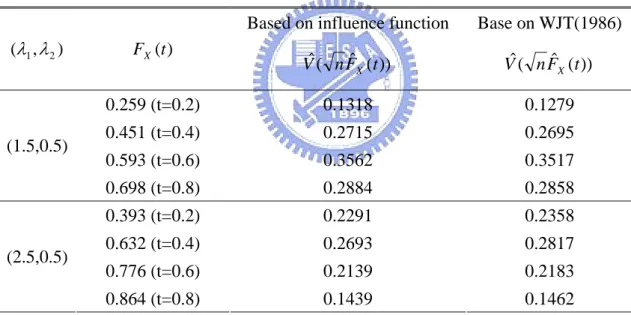
The asymptotic expression via influence functions has significant advantage when we study the joint behavior of (FˆX,SˆY). Now we fix a point (x,y)∈RU. Based on the

asymptotic linear expression,

⎥ ⎦ ⎤ ⎢ ⎣ ⎡ ⎟⎟ ⎠ ⎞ ⎜⎜ ⎝ ⎛ ⎟⎟ ⎠ ⎞ ⎜⎜ ⎝ ⎛ ⎯→ ⎯ ⎥ ⎦ ⎤ ⎢ ⎣ ⎡ − − X XY XY Y d X X Y Y V V V V N x F x F y S y S n 0 0 ) ( ) ( ˆ ) ( ) ( ˆ . ) , (λ₁ λ₂ F_X(t)

Based on influence function )) ( ˆ ( ˆ _{nF t} V _X Base on WJT(1986) )) ( ˆ ( ˆ _{nF t} V _X 0.259 (t=0.2) 0.1957 0.1953 0.451 (t=0.4) 0.2890 0.2871 0.593 (t=0.6) 0.3057 0.3119 (1.5,0.5) 0.698 (t=0.8) 0.3273 0.3212 0.393 (t=0.2) 0.2567 0.2549 0.632 (t=0.4) 0.2695 0.2725 0.776 (t=0.6) 0.2144 0.2170 (2.5,0.5) 0.864 (t=0.8) 0.1861 0.1878 ) , (λ1 λ2 FX(t)

Based on influence function )) ( ˆ ( ˆ _{nF t} V X Base on WJT(1986) )) ( ˆ ( ˆ _{nF t} V X 0.259 (t=0.2) 0.1318 0.1279 0.451 (t=0.4) 0.2715 0.2695 0.593 (t=0.6) 0.3562 0.3517 (1.5,0.5) 0.698 (t=0.8) 0.2884 0.2858 0.393 (t=0.2) 0.2291 0.2358 0.632 (t=0.4) 0.2693 0.2817 0.776 (t=0.6) 0.2139 0.2183 (2.5,0.5) 0.864 (t=0.8) 0.1439 0.1462

The terms in the covariance matrix can be estimated as follows. ] ) ; , ( [ ) ( ) ; , ( ˆ ) ( ˆ 2 2 2 2 x Y X L E x F V x Y X L n x F X X X i i i X X

∑

→ = , ] ) ; , ( [ ) ( ) ; , ( ˆ ) ( ˆ 2 2 2 2 y Y X L E y S V y Y X L n y S Y Y Y i i i Y Y

∑

→ = , and )]. ; , ( ) ; , ( [ ) ; , ( ˆ ) ; , ( ˆ ) ( ˆ ) ( ˆ x Y X L y Y X L E V x Y X L y Y X L n y S x F Y X XY i i i X i i Y Y X

∑

→ =

Using the delta method, we obtain

) , 0 ( )) ( ) ( ) ( ˆ ) ( ˆ (S y F x S y F x N V n _{Y X} − _{Y X} ⎯⎯→d ,

where the asymptotic variance is

X Y XY Y X Y X x V F x S yV S y V F V = ( )2 +2 ( ) ( ) + ( )2 .

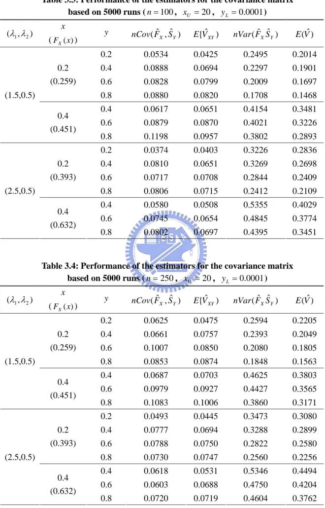
Simulation studies confirm the satisfactory results about the proposed estimators of V_XY and

Table 3.3: Performance of the estimators for the covariance matrix based on 5000 runs (n=100, x_U =20, y_L =0.0001) ) , (λ1 λ2 x (F_X(x)) y ) ˆ , ˆ (F_X S_Y nCov E{Vˆ_XY) nVar(Fˆ_XSˆ_Y) E(Vˆ) 0.2 0.0534 0.0425 0.2495 0.2014 0.4 0.0888 0.0694 0.2297 0.1901 0.6 0.0828 0.0799 0.2009 0.1697 0.2 (0.259) 0.8 0.0880 0.0820 0.1708 0.1468 0.4 0.0617 0.0651 0.4154 0.3481 0.6 0.0879 0.0870 0.4021 0.3226 (1.5,0.5) 0.4 (0.451) 0.8 0.1198 0.0957 0.3802 0.2893 0.2 0.0374 0.0403 0.3226 0.2836 0.4 0.0810 0.0651 0.3269 0.2698 0.6 0.0717 0.0708 0.2844 0.2409 0.2 (0.393) 0.8 0.0806 0.0715 0.2412 0.2109 0.4 0.0580 0.0508 0.5355 0.4029 0.6 0.0745 0.0654 0.4845 0.3774 (2.5,0.5) 0.4 (0.632) 0.8 0.0802 0.0697 0.4395 0.3451

Table 3.4: Performance of the estimators for the covariance matrix

based on 5000 runs (n=250, x_U =20, y_L =0.0001) ) , (λ1 λ2 x (F_X(x)) y ) ˆ , ˆ (F_X S_Y nCov E{Vˆ_XY) nVar(Fˆ_XSˆ_Y) E(Vˆ) 0.2 0.0625 0.0475 0.2594 0.2205 0.4 0.0661 0.0757 0.2393 0.2049 0.6 0.1007 0.0850 0.2080 0.1805 0.2 (0.259) 0.8 0.0853 0.0874 0.1848 0.1563 0.4 0.0687 0.0703 0.4625 0.3803 0.6 0.0979 0.0927 0.4427 0.3565 (1.5,0.5) 0.4 (0.451) 0.8 0.1083 0.1006 0.3860 0.3171 0.2 0.0493 0.0445 0.3473 0.3080 0.4 0.0777 0.0694 0.3288 0.2899 0.6 0.0788 0.0750 0.2822 0.2580 0.2 (0.393) 0.8 0.0730 0.0747 0.2560 0.2256 0.4 0.0618 0.0531 0.5346 0.4494 0.6 0.0603 0.0688 0.4750 0.4204 (2.5,0.5) 0.4 (0.632) 0.8 0.0720 0.0719 0.4604 0.3762