用於HEVC編碼單元之快速決策演算法 與 結合移動向量與DCT之H.264編碼器優化

國

立

交

通

大

學

電子工程學系 電子研究所

碩 士 論 文

用於HEVC編碼單元之快速決策演算法 與

結合移動向量與DCT之H.264編碼器優化

Fast HEVC Coding Unit Decision Algorithm and

Combined MV and DCT Optimization for

H.264/AVC Codec

研 究 生：許維哲

指導教授：杭學鳴 博士

用於HEVC編碼單元之快速決策演算法 與

結合移動向量與DCT之H.264編碼器優化

Fast HEVC Coding Unit Decision Algorithm and

Combined MV and DCT Optimization for

H.264/AVC Codec

研 究 生：許維哲 Student：Wei-Jhe Hsu

指導教授：杭學鳴 博士 Advisor：Dr. Hsueh-Ming Hang

國 立 交 通 大 學

電子工程學系 電子研究所

碩 士 論 文

A Thesis

Submitted to Department of Electronics Engineering and Institute of Electronics

College of Electrical and Computer Engineering National Chiao Tung University

In Partial Fulfillment of the Requirements for the Degree of

Master of Science in

Electronics Engineering

July 2012

Hsinchu, Taiwan, Republic of China

用於

HEVC 編碼單元之快速決策演算法 與

結合移動向量與

DCT 之 H.264 編碼器優化

研究生 : 許維哲 指導教授 : 杭學鳴 博士 國立交通大學 電子工程學系 電子研究所碩士班

摘要

由於高解析度影像應用的需求，視訊編碼在3C 產品中是不可或缺的技術，例如行

動電話、高畫質電視、藍光光碟機。進階視訊編碼(Advanced Video Coding, AVC/H.264) 是目前商業產品中，廣泛採用的壓縮標準格式。為了達到更高的編碼效率，國際組織 JCT-VC 正在進行下一代標準的制定，即高效率視訊編碼(High Efficiency Video Coding, HEVC) 。 相較於進階視訊編碼，雖然高效率視訊編碼的複雜度提升許多，但是在相似 的影像品質下，可以增加近一倍的壓縮效率。

此論文包含兩個研究主題：第一個主題是改善進階視訊編碼中，整數精確度的移動 估測以增進編碼效能；第二個主題是關於高效率視訊編碼的編碼單元(Coding Unit, CU) 大小的快速決策，以達到降低編碼器複雜度的目標。在進階視訊編碼中，整數移動估測 的失真項，是以區塊之絕對誤差總和(The Sum of the Absolute Distortion, SAD)來 計算，但是此方法並不能完全反應最後結果的失真。為了在相似的畫面品質下，進一步 節省位元率，我們提出迭代的位元率-失真(Rate-Distortion, R-D)計算方式，以選擇 較佳的移動向量。我們將此演算法實現於 JM18.0，用許多組 MPEG 測試影像來檢驗此方 法的效能，並將執行結果和原始 JM 做法的結果進行比較。雖然 JM18.0 是發展已久的優 化編碼器，我們仍可從中節省 1.1%至 4.2%的位元率，但代價是增加 45%的運算複雜度。

另一方面，高效率視訊編碼在傳統的編碼流程中，增加了編碼單元四元分割樹的構 造。彈性的編碼單元設計提升了編碼效率，但相較於進階視訊編碼傳統的巨區塊 (Macroblock, MB)結構而言，編碼複雜度提升不少。因此我們設計快速演算法以有效率 地建造出編碼單元四元分割樹，其中演算法包括分裂決策、終止決策。這些快速編碼單 元大小決策參考週遭相關的編碼單元之切割資訊以進行判斷。此外，我們設計額外的工 具以增進我們提出的演算法效能，其中包含畫面層級加速控制和跳過決策後的快速預測 單元判斷。最後，我們分析提出的快速演算法，並和 HM5.0 中的兩種快速演算法進行比 較，以找出有效率的結合方法。相較於 HM5.0 的原始設定，我們提出的快速演算法，經 過多組高解析度的影像測試，可以節省高達 49%的整體編碼時間，但平均損失 0.06dB 的峰值信噪比(PSNR)。

Fast HEVC Coding Unit Decision Algorithm and

Combined MV and DCT Optimization for H.264/AVC

Codec

Student : Wei-Jhe Hsu Advisor : Dr. Hsueh-Ming Hang

Department of Electronic Engineering & Institute of Electronics National Chiao Tung University

Abstract

With the growing demand for high resolution video applications, video coding is an indispensable element in many 3C products, such as mobile phone, DTV, and BD player. Today, Advanced Video coding (AVC/H.264) is one of the most popular video formats in commercial applications. Aiming at higher compression efficiency, the international JCT-VC is currently developing the next generation standard, High Efficiency Video Coding (HEVC). With a much higher encoder complexity, HEVC is able to achieve a 50% bitrate reduction compared to H.264/AVC.

This thesis has two topics, one is the enhanced motion estimation (ME) for AVC/H.264 and the other is the fast coding unit (CU) decision for HEVC. In H.264, the sum of the absolute difference (SAD) is used as the distortion term in ME, but it does not reflect the final coding distortion. To achieve further bitrate reduction, we propose an enhanced motion vector selection method based on the iterative R-D calculation. We compare the proposed method with the original H.264/AVC JM18.0 reference software on several MPEG test sequences. Although

JM18.0 is a highly optimized scheme, we can still obtain a BD-rate improvement from 1.1% to 4.2% but with additional 45% complexity increase.

In HEVC, the CU quadtree structure is added to the traditional fixed size macroblock. With flexible CU size selection, the coding efficiency increases but the complexity of HEVC becomes much higher than that of AVC/H.264 fixed macroblock (MB) structure. To reduce computational complexity, we propose a fast algorithm, which includes the splitting decision and the termination decision, in building the CU quadtree. The fast CU size decision of the current CU makes use of the size information of its neighboring CUs. Furthermore, we design the additional tools to enhance the performance of the proposed algorithm. The additional tools include the frame level acceleration and the fast PU size decision after the splitting decision. At the end, we compare it with the existing fast algorithms in HM5.0 and find an efficient way to blend them together. In comparison to the original HM5.0, our method saves the overall encoding time up to 49% with 0.06 dB average PSNR drop.

誌謝

鳳凰花開，又到了畢業的季節。而我也終於拿到了我的碩士學位。當初，剛開始進 入交大電子研究所就讀時，因為是跨領域 (從固態換系統)，系統組的老師實在難找， 領域也選擇了許久。幸運地，杭學鳴教授願意指導我。老師開啟了我的學術之路，提供 了充足的研究環境和有趣的研究題目，使我心中名為研究生的種子慢慢地發芽、成長； 老師豐富的學術知識和謙遜的人生態度更是我學習的目標，在此誠摯地感謝我的指導老 師杭學鳴教授。 在我碩士兩年的求學之旅中，最有回憶的地方就是 Commlab。在這邊，我接觸到許 多強者學長：感謝朝雄學長辛苦地管理實驗室，並且常和我分享研究的甘苦；謝謝峻利 學長和宸銜學長平時跟我討論研究和課業；感謝書緯學長教我如何看 CODE、改 CODE， 在學長畢業後還一直熱心地提供我 HEVC 方面的技術支援；謝謝崇豪學長，讓我了解做 研究該有的熱情；謝謝鴻志學長，您留下的 MATLAB 教材非常的實用；感謝家揚學長在 我做 AVC 計劃時，教我如何下手改 CODE；謝謝彰哲學長和柏森學長在我找工作時，給予 我人生道路和工作態度的建議；學長們無論在研究、課業、人生態度都給我很大的啟示 和幫助。另外，我也在這邊碰到了許多有趣的同學：感謝讀修從我準備考研究所開始， 就不斷地幫助我解決數學上的問題；謝謝義文平時約我去健身，鍛鍊身體兼紓發壓力； 感謝士傑與我一起準備七月的口試，讓我得以順利地通過口試。Commlab 的人、事、物

在這兩年來給予我很大的幫助，我在此由衷地感謝。這邊也特別感謝 MAPL 的俊吉學長 和彥宇，在我口試之前，幫我確認基本的想法，消除我緊張的心情。 最後我想感謝的是交大和我的家人。我在交大就讀的六年之中，我從交大得到許多 重要的東西和回憶，在此特別感謝母校。感謝我的家人，總是在背後支持著我，一路走 來有他們的親情和支持，我才能有現在的成就。 將此篇論文獻給所有關心我的人，因 為有你們，我會盡力讓自己變得更好。 維哲 7/20 於 Commlab 筆

CONTENTS

摘要………...………...i Abstraction...………...iii 誌謝………...………..v CONTENTS...vii LIST OF FIGURES ... x

LIST OF TABLES ... xii

Chapter 1 Introduction ... 1

1.1 Research Contributions ... 2

1.2 Thesis Organization ... 3

Chapter 2 Overview of H.264/AVC and HEVC ... 4

2.1 Advanced Video Coding ... 4

2.1.1 H.264 Architecture ... 5

2.1.2 Basic Coding Tools ... 5

2.1.2.1 Intra prediction ... 6

2.1.2.2 Inter Prediction ... 6

2.1.2.3 Transform and Quantization ... 7

2.1.2.4 Deblocking Filter ... 7

2.1.2.5 Entropy Coding ... 8

2.1.3 Encoder Control ... 8

2.1.3.1 Searching for Optimal Motion Vector ... 10

2.1.3.2 Selection for the Best Mode ... 10

2.2 High Efficiency Video Coding ... 11

2.2.1 Coding Unit Definition ... 12

2.2.1.2 Prediction Unit ... 13

2.2.1.3 Transform Unit ... 14

2.2.2 Enhanced Coding Tools ... 15

2.2.2.1 Intra prediction ... 17

2.2.2.2 Inter Prediction ... 17

2.2.2.3 Transform and Quantization ... 18

2.2.2.4 Loop Filter ... 18

2.2.2.5 Entropy Coding ... 19

2.3 Experiment Conditions ... 19

Chapter 3 Nested Quadtree Coding Unit ... 22

3.1 Overview of Coding Unit Quadtree Structure ... 22

3.1.1 Partition Decision Flow of Nested Quadtree CU ... 23

3.1.2 Existing fast algorithms for Partition Decision Flow in HM5.0 ... 25

3.2 Analysis of Nested CU Quadtree Structure ... 29

Chapter 4 Fast CU Size Decision Algorithm Design ... 32

4.1 Problem Formulation and Design Goal ... 32

4.2 Related Work ... 33

4.3 Core Ideas of Fast CU Size Decision ... 34

4.3.1 Splitting Decision ... 36

4.3.2 Termination Decision ... 37

4.3.3 Basic Fast CU Size Decision Scheme ... 38

4.4 Additional Tools ... 39

4.4.1 Frame Level Parameter Control ... 40

4.4.2 LCU Level Parameter Control with Error-Bound ... 45

4.5 Overview of the Overall Proposed Algorithm ... 55

Chapter 5 HEVC Experiments and Discussions ... 57

5.1 Performance Measure ... 57

5.2 Experimental Results and Discussions ... 59

5.2.1 Fast CU Size Decision ... 59

5.2.2 Comparison with ECU/CFM ... 70

5.2.3 Combined Fast CU Size Decision with ECU/CFM ... 72

Chapter 6 Combined MV and DCT Optimization for H.264/AVC Codec ... 76

6.1 MV Refinement with DCT result ... 76

6.2 Modified MV Selection Scheme ... 78

6.3 AVC/H.264 Experimental Results and Discussions ... 81

Chapter 7 Conclusions and Future Work ... 88

7.1 Conclusions ... 88

7.2 Future Work ... 89

LIST OF FIGURES

Fig. 1 An H.264/AVC encoder ... 5

Fig. 2 R-D optimization for selecting MV and mode ... 9

Fig. 3 An HEVC encoder ... 12

Fig. 4 An Example of a nested quadtree structure [8] ... 15

Fig. 5 Possible PUs in low complexity setting ... 15

Fig. 6 An example of nested CU quadtree structure (Vidyo1, Frame 2, QP=32) ... 23

Fig. 7 A G-BFOS example. ... 25

Fig. 8 An example of ECU [18] ... 28

Fig. 9 Program flow of CFM ... 29

Fig. 10 PU execution order in CU in the low-complexity setting ... 29

Fig. 11 Data representation of splitting information ... 34

Fig. 12 Reference CUs and the current CU ... 35

Fig. 13 An example of splitting decision ... 36

Fig. 14 An example of termination decision... 38

Fig. 15 Flowchart of basic fast CU size decision algorithm ... 39

Fig. 16 R-D curve of Basketball ... 41

Fig. 17 Example of Nc=3 ... 42

Fig. 18 Experiment for choosing N_c ... 44

Fig. 19 R-D curve of Basketball with Nc control ... 45

Fig. 20 Error bound (3%) for SAD ... 47

Fig. 21 Second order curve fitting for error bound (3%) ... 47

Fig. 22 Probability density distribution of SAD of “Kimono” ... 51

Fig. 25 An example of 2NxN/Nx2N Decision in depth 2 ... 54

Fig. 26 Flowchart of overall proposed algorithm for processing an LCU ... 56

Fig. 27 CU distribution of the 9th frame of BQsquare (QP=32) ... 64

Fig. 28 CU distribution of the 9th frame of Vidyo1 (QP=32) ... 65

Fig. 29 CU distribution of the 9th frame of BQTerrence (QP=22) ... 65

Fig. 30 Pie chart of depth amount ratio of BQsquare (QP=32) ... 66

Fig. 31 Pie chart of depth amount ratio of Vidyo1 (QP=32) ... 67

Fig. 32 Average depth of Vidyo1 (QP=37) ... 68

Fig. 33 Average depth of BQTerrence (QP=22) ... 68

Fig. 34 R-D curve of Basketball in Table 26 ... 73

Fig. 35 Difference between the JM-encoded and our proposed method ... 79

Fig. 36 Spatial domain: The residual MBs of Inter-16x16 mode on the second frame. .. 79

Fig. 37 Frequency domain: The transformed and quantized residual MBs of Fig.4. ... 80

Fig. 38 Flowchart of the combined ME and DCT algorithm ... 81

LIST OF TABLES

Table 1 Structure of Tools in HM 5.0 Configures [9] ... 16

Table 2 Experiment Conditions ... 20

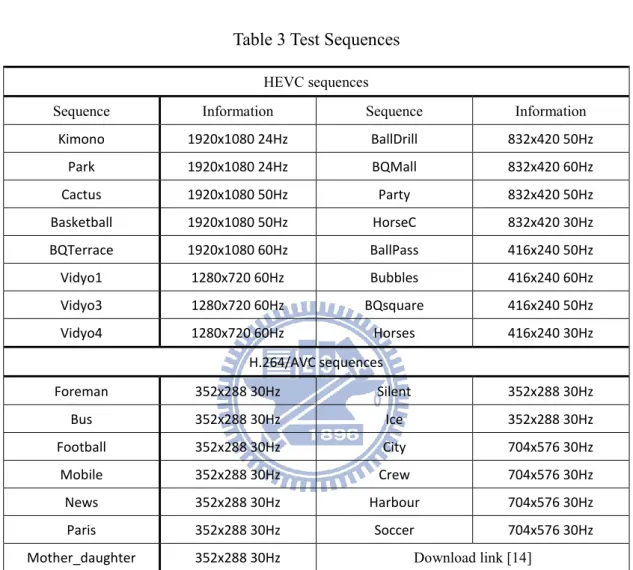
Table 3 Test Sequences ... 21

Table 4 Time percentage of “xCompressCU.cpp” in HM5.0 ... 30

Table 5 Comparison of 64/4 CU structure and 16/2 CU structure ... 31

Table 6 Performance of the basic fast CU decision algorithm ... 41

Table 7 Specified QP versus Nc ... 43

Table 8 BD-performance and time reduction ratio of limited Nc ... 43

Table 9 PSNR and bits measurements at QP=32 ... 44

Table 10 Specified QP versus error bound (3%) ... 48

Table 11 BD-performance and time reduction ratio with 3% error bound ... 48

Table 12 Simulation result with 3% error bound with 64 frames per sequence ... 48

Table 13 Simulation result without error bound with 64 frames per sequence ... 49

Table 14 Comparison of different ratios of error bound ... 50

Table 15 Performance for schemes with and without 2NxN/Nx2N decision ... 55

Table 16 Performance of the overall proposed algorithm (64 frames/sequence) ... 60

Table 17 Performance of the overall proposed algorithm (100 frames/sequence) ... 60

Table 18 Depth percentage (QP is 32) ... 62

Table 19 Depth percentage of the 10th frame in low resolution sequences (QP=37) ... 62

Table 20 Depth percentage of the 10th frame in HD sequences (QP=37) ... 62

Table 21 Time reduction ratio analysis of Vidyo1 and BQsquare ... 63

Table 22 Depth percentage of BQTerrence (QP=22) ... 64

Table 25 Simulation results of ECU and CFM with our low delay_P loco setting ... 71

Table 26 Simulation result of ECU, CFM, and our proposed algorithm ... 72

Table 27 Results of the adaptively combined fast algorithm with ECU and CFM ... 74

Table 28 R-D performance of our proposed algorithm (QP= 22) ... 75

Table 29 R-D Comparison for FOREMAN in P slices ... 83

Table 30 Modes and Motion Info Bits/Frame ... 83

Table 31 BD Rate Improvement in P Slices of all Sequences ... 85

Table 32 Final MV Choice from Candidate MVs (Percentages) ... 86

Chapter 1 Introduction

Video coding plays an important role in the commercial products, and its techniques have been developed during the past 20 years. The matured video compression technique is adopted by many applications, such as television, digital camera, mobile communication, and video recording devices, to store and transmit a large amount of video data. For the better visual quality and the bitrate reduction, the international standard committee is still specifying new standards, and many researchers are still looking for better algorithms. The main stream of video coding in recently years is AVC/H.264. HEVC is the next generation standard that is still in progress.

In this thesis, we study both AVC/H.264 and HEVC. In AVC/H.264, we study the transform effect on the motion vector search and design an iterative scheme to improve the overall coding performance. In HEVC, the coding unit (CU) has flexible sizes. In general, the HEVC encoder uses large CU in the stationary or smooth areas particularly at low bitrates. It uses small CUs in the texture areas at the high bitrates. Although HEVC has a better coding performance, it takes a large amount of the complexity to decide the best CU size. Therefore, we want to design a fast algorithm in deciding CU size to reduce calculations.

1.1

Research Contributions

The main contributions of the HEVC part are the development and the analysis of the fast CU decision. Our proposed algorithm achieves up to 49% encoding time reduction, or equivalently, about 2x speed up. On the other hand, the contribution of the AVC part is designing a method to improve compression efficiency by modifying the motion selection process. Our proposed iterative scheme saves up to 4.2% bitrate usage and it retains the video quality. The major contributions in this thesis are listed as below.

1. Develop a fast CU size algorithm for HEVC based on the size information of the neighboring CUs. The fast algorithm includes splitting decision and termination decision.

2. Propose additional tools to further enhance video quality or to reduce complexity.

3. Compare and combine our proposed method to the existing fast algorithms in HM5.0. We investigate their advantages and disadvantages, and find an efficient way to combine them together.

1.2

Thesis Organization

The rest of this thesis is organized as follows. Chapter 2 gives a brief overview of the state-of-the-art encoders, AVC/H.264 and HEVC. We describe their work flows, their basic operations, and the HEVC advanced coding features. The thesis has two parts: the HEVC part is from Chapter 3 to Chapter 5, and Chapter 6 is the AVC part. In Chapter 3, we describe the CU quadtree structure in HEVC, and introduce the fast algorithms in HM5.0. In Chapter 4, we describe the proposed fast CU size decision algorithm in detail. Then, we design several compensated schemes to improve the original fast algorithm. Chapter 5 presents the simulation results of our scheme and discusses the possible combinations with the existing fast scheme. The second part of this thesis is about AVC/H.264 motion vector search in Chapter 6. Finally, Chapter 7 summarizes our work.

Chapter 2 Overview of H.264/AVC and HEVC

In 1993, the ITU-T Video Coding Experts Group (VCEG) started a long-term project (H.26L). After about ten years of development, the project led to the well-known H.264 standard [1]. The final stage of developing the H.264/MPEG Advanced Video Coding (AVC) standard was carried out by the ITU and ISO/MPEG Joint Video Team (JVT) in 2003. In the past a couple of years, MPEG and VCEG collaborate again to form the Joint Collaborative Team on Video Coding (JCT-VC). With the demand of high-resolution video applications, JCT-VC is currently specifying the next generation video standard, High Efficiency Video Coding (HEVC), which aims to achieve about 50% bit-rate reduction compared to H.264/AVC. And HEVC is expected to be finalized in 2012. For more information about the progress of AVC and HEVC, please refer to [2].

2.1

Advanced Video Coding

Basically, the H.264/AVC standard has a video coding structure similar to that of the prior video coding standards, which is known as the “hybrid coding scheme” [3]. It uses transform coding to code the motion compensated prediction errors. The basic processing unit is macroblock (MB), corresponding to a 16 × 16 -pixel square region of a frame. In this section, we will introduce the fundamental concept of H.264/AVC. For more details, please

refer to [1], [4].

2.1.1 H.264 Architecture

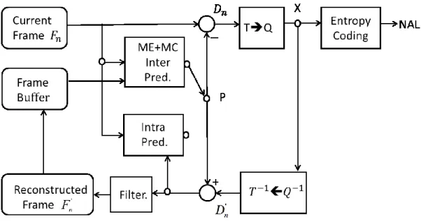
Fig. 1 shows a typical H.264/AVC encoder. The encoder includes two data paths, an encoding path (left to right) and a reconstruction path (right to left). An input video frame Fn

is processed in the unit of MB. A coded MB may belong to an I-MB (intra-coded), P-MB (predictive-coded), and B-MB (bi-directional predictive-coded).

Fig. 1 An H.264/AVC encoder

2.1.2 Basic Coding Tools

In Fig. 1, a prediction block P is formed by intra-prediction or inter-prediction. A residual block Dn is produced by subtracting the prediction block P from the current block.

and it is quantized toX . The quantized transform coefficients are reordered, and then are entropy-coded. The above coding tools are explained in detail in the following subsections.

2.1.2.1 Intra prediction

Because the correlation between the neighboring blocks within a video frame is extremely high, the encoder, which uses the intra-prediction, can reduce the spatial redundancy. In the intra modes, a prediction block P is generated based on the neighboring blocks (top-left, top, top-right, and left.), which have been encoded and reconstructed. There are four optional intra-prediction modes for a 16 × 16 luma block, and nine modes for each 4 × 4 luma block. A special intra coding mode, I_PCM, transmits the image samples directly (without prediction or transform).

2.1.2.2 Inter Prediction

For video sequences at high frame rate, the nearby frames are generally similar. By using the inter-prediction technique to transmit the difference between successive frames, the temporal redundancy could be reduced. The P and B MBs may be coded in one of motion-compensation (MC) modes. Motion compensated prediction based on one or more reference pictures produces the predictionP. An inter-mode MB can be partitioned into various sizes corresponding to the SKIP mode, INTER-16×16, INTER-8×16, INTER-16×8, and INTER-8×8 modes, and an 8×8 sub-MB mode can be further divided into smaller partitions

with block sizes of 8×4, 4×8, 4×4 blocks. Motion estimation (ME) is a key step in inter-prediction. The partitioned block inside an inter-mode MB is predicted from the same size region in the reference pictures. The vector from the current frame block pointing to the best matching region in the referenced frame is the so-called motion vector (MV).

2.1.2.3 Transform and Quantization

Due to the inter-pixel redundancy in the residual block, the encoder transforms the spatial domain pixels to the frequency domain coefficients to compress its original redundant information. The discrete cosine transformation (DCT) is a general tool in the state-of-the-art video encoder. In AVC/H.264, there are two variable size transforms: 4×4 and 8×8. To increase their computational speeds, they are implemented in the butterfly structure that uses addition, bit-shift, and a few multiplication operations. The DCT coefficients of a residual block should be processed by reordering (zig-zag scanning), scaling, and rounding (quantization). The Quantization parameter (QP) ranges from 0 to 51. With an increment of 6 in QP, the quantization step becomes double.

2.1.2.4 Deblocking Filter

The deblocking filter is designed for eliminating the blocking artifacts on the boundaries, which are caused by the block-based transform with a coarse quantization and by the MC prediction in which the interpolated data are derived from different regions of multiple

reference frames. The filter is applied to each decoded MB to reduce blocking distortion, and the encoder stores the filtered MB in the reconstruction frame to be used as the reference frame in the future. The deblocking filter is an important coding tool for inter-prediction.

2.1.2.5 Entropy Coding

At the slice layer level and below, the syntax elements are encoded either by the variable length coding tool (VLC) or by the context-adaptive arithmetic coding tool (CABAC). In VLC, a quantized DCT block is coded by using the context-adaptive variable length coding (CAVLC) scheme, and the other data units are coded by using Exp-Golomb codes. The tables of CAVLC are designed to match the corresponding conditional probability. The context adaptive feature of CABAC can be more efficient became it is adaptive to the statistics of previously encoded data. Generally, CAVLC has low complexity, and CABAC has better efficiency.

2.1.3 Encoder Control

The H.264/AVC standard provides only the syntax of bit-stream and the decoder structure. Therefore, we need to design and to control the encoding process in our preferred way. How to decide the coding parameters is a key to achieve video compression efficiency. The H.264 coding parameters include MVs, quantization levels, and MB modes. The same encoder structure with different coding parameters will affect the R-D efficiency of the produced bit-stream.

The general R-D cost function for video coding is presented by (1). In (1), symbol D denotes distortion, which is often the absolute difference between the processed image block and the original block. Symbol R means rate, which is the bits needed to send the processed information. According to the information theory, we can fix R first and then minimize D. We can combine D and R together to form the total cost J. Mathematically, we can convert this constrained optimization problem to a non-constrained form, the so-called Lagrange cost function in (1). How to select the optimal Lagrange multiplier  is a difficult problem in practice, and for more details, please refer to [5], [6].

J  D R (1)

A traditional H.264/AVC encoder splits the optimization of the cost function for the inter modes into two parts as illustrated in Fig. 2. The first part is finding the optimal MV, and second part is choosing the best mode, block size etc.

Motion Vectors Selection Mode Selection Entropy Coding Controller of RD Optimization MB (2) (4) _Rate Mode MV

2.1.3.1 Searching for Optimal Motion Vector

A traditional H.264/AVC encoder splits the optimization of the cost function for the inter modes into two parts. In the first part, the encoder finds the MVs with the optimum residual distortion and the MV coding bits. Based on the motion R-D cost function (2), [3], the motion estimation step finds the vector with the smallest cost for various block sizes. Given the current and the reference frames and the Lagrange multipliermotion, the ME operation for a

partition block si is to minimize (2) to find the best MV.

( , ) ( , ),

motion motion i motion motion i

J D s m  R s m (2)

where m is the set consists of all possible vectors ( ,m m m_{x y}, _t), in which m_x is the MV horizontal component, and m_y is the vertical component, m_t is time difference. R_motionis the number of bits for transmitting MV, and Dmotion is the distortion term given by

( , ) ( , ) ( , , ) ( , , ) i p motion i x y t x y s D s m pixel x y t pixel x m y m t m  



    (3)

To speed-up the ME process, we usually choosep 1, and (3) becomes the sum of the absolute difference (SAD). The symbols, xandy, are the pixel location in a block. It should

be noted that the state-of-the-art encoder often uses hadamard measure for fractional ME for coding efficiency, and the detail is describe in section 6.1.

2.1.3.2 Selection for the Best Mode

motion-compensated residual error signals, and then we choose the best MB coding mode. With the given Lagrange parameter mode and the quantized parameterQ, the coding mode

of MB (S) is decided by minimizing the following R-D cost function [3],





mode ( , ) | ,k mode  REC( , | )k mode REC( , | ),k

J S I Q D S I Q R S I Q (4)

where Ik represents a legitimate mode. For example, k possible modes for P-slice in

H.264/AVC are Intra-16×16, Intra 4×4, SKIP mode, INTER-16×16, INTER-8×16, INTER- 16×8, INTER- 8×8 modes.DRECis the distortion between the reconstructed MB and the

original one, and it is usually measured in the sum of the squared difference (SSD), p=2 in (3).

REC

R denotes the rate after entropy coding for a MB. Although the calculated cost function is

an approximation, it reflects the rate-distortion efficiency reliably.

2.2

High Efficiency Video Coding

A joint call-for-Proposal (CfP) for HEVC was issued by JCT-VC in January 2010, and 27 proposals in response of the CfP were submitted with their test material. The promising results were reported in [7], and the proposed scheme [8] from Heinrich Hertz Institute (HHI) was ranked among the five best performing proposals. For its wonderful performance, most of its design elements were selected to specify a first model of the initialed HEVC standardization project. The project is still in progress, and HEVC is expected to achieve excellent coding performance on high resolution video with low delay and low complexity.

Fig. 3 shows the HEVC encoder structure. Although HEVC has a similar structure to the H.264/AVC architecture, there are some significant innovations in HEVC. The innovations of re-definition of coding units and the enhancement on coding tools offer remarkable compression efficiency.

Fig. 3 An HEVC encoder

2.2.1 Coding Unit Definition

In H.264/AVC, the basic processing unit is called MB, which is expanded to what we called a coding tree block (CTB). For flexibility and efficiency, the basic coding units in HEVC have variable sizes with various resolutions. They are CU (Coding Units), PU (Prediction Units), and TU (Transform Units). A CTB in HEVC which covers 2Nmax2Nmax

subdivided for CUs, corresponding PUs and TUs. The concept of decomposing MB into three different units allows each to be optimized independently, which brings high adaption to enhance the performance of each coding tools. The definition and details of three units in the HEVC encoder [9] are given in the following sub sections.

2.2.1.1 Coding Unit

A basic unit of HEVC, referred as CU, is a square region of a picture, and it may contain several PUs and TUs. An input processing frame is divided into slices, and each slice is composed of CTBs, which are also called largest coding units (LCUs). Dividing a picture into LCUs and further recursively subdividing each CUs into 4 smaller CUs with half width and half height is the so called nested quadtree structure as shown in Fig. 4 (with solid lines). Both the block sizes and the block coding parameters such as maximum allowed depth will be specified in the sequence parameter set (SPS) or the slice header.

2.2.1.2 Prediction Unit

PU is defined only for the leaf node of CU in each depth level, and PUs have various partitions for prediction. They are confined within its CU node with a shape of square or rectangular, and for some cases the prediction units are asymmetric in CU as list in Table 1. The prediction ways are similar to the prediction methods of H.264/AVC, which can be the skip, the intra, or the inter modes. In Fig. 5, we can see all the possible PUs for each

prediction mode in low complexity setting. The information related prediction such as the PU splitting types, the prediction modes, the intra prediction direction, the motion vector difference (MVD), and the corresponding referenced frame indices are transmitted in PU level.

2.2.1.3 Transform Unit

TU is a basic unit of residual coding, including transform and quantization. The TUs are aligned within their corresponding CU, and the size of TUs is variable which is not constrained by boundaries of PU. In HM5.0, the NSQT is added, that is, the shape of TU has not to be square, and it may be rectangular. The splitting flag and transform coefficients are specified in TU level.

The tree structure of CU or TU splits from top to down, but the optimal structure is decided by G-BFOS algorithm [10], [11]. The algorithm makes pruning decision from bottom to up, which reduces much computational complexity, and we will describe the detail part in the next chapter. The coding tree blocks for TU are illustrated by Fig. 4 (with dashed line). More details of the encoder controller for HEVC are described in chapter 3. An Example of a nested quadtree structure (right part) for dividing a given coding tree block (left part) in Fig. 4. The order of parsing the coding blocks follows their labeling in alphabetical order.

Fig. 4 An Example of a nested quadtree structure [8] 2NxN 2Nx2N Nx2N NxN 2Nx2N 2Nx2N NxN Skip Intra Inter

Intra NxN is only used as 2N=8 Inter NxN is close originally.

Fig. 5 Possible PUs in low complexity setting

2.2.2 Enhanced Coding Tools

After H.264/AVC standard was defined, people tried to propose algorithm to improve it. As time goes by, people notice that some modifications on the existing tools and many newly proposed tools provide a certain amount of improvement. Therefore, many adaptive and novel

tools are adopted in the current HEVC model compared to H.264/AVC. With the development of HEVC standardization project, JCT-VC adds useful tools, refines the existing tools, and removes inferior tools in the model [12]. A summary list of the tools that are included in HM5.0 is provided in Table 1 below.

Table 1 Structure of Tools in HM 5.0 Configures [9]

High Efficiency Configuration Low Complexity Configuration

Coding units, Prediction units, and Transform units:

Coding unit quadtree structure

(square coding unit block sizes 2Nx2N, for N=4, 8, 16, 32; i.e., up to 64x64 luma samples in size)

Prediction units (for coding unit size 2Nx2N: (1) for Inter, 2Nx2N, 2NxN, Nx2N, and,

for N>4, also 2Nx(N/2+3N/2) & (N/2+3N/2)x2N;

(2) for Intra, only 2Nx2N and, for N=4, also NxN)

Prediction units (for coding unit size 2Nx2N: (1) for Inter, 2Nx2N, 2NxN, Nx2N; (2) for Intra, only 2Nx2N and, for N=4, also NxN)

Transform unit tree structure within coding unit (maximum of 3 levels)

Transform block size of 4x4 to 32x32 samples (always square for Intra; also non-square 4x16,

16x4, 8x32, 32x8 for Inter)

Transform block size of 4x4 to 32x32 samples (always square )

Spatial Signal Transformation and PCM Representation:

DCT-like integer block transform;

for Intra also a DST-based integer block transform (selected based on the intra prediction mode)

Transforms can cross prediction unit boundaries for Inter; not for Intra PCM coding with worst-case bit usage limit

Intra-picture Prediction:

Angular intra prediction (17 directions for 4x4, 3 directions for 64x64, 34 directions for others) Planar intra prediction

Chroma intra prediction separate from or using luma samples

Inter-picture Prediction:

Luma motion compensation interpolation: 1/4 sample precision, 8x8 separable with 6 bit tap values

Chroma motion compensation interpolation: 1/8 sample precision, 4x4 separable with 6 bit tap values

Advanced motion vector prediction with motion vector “competition” and “merging”

Entropy Coding:

Context adaptive binary arithmetic entropy coding

RDOQ on RDOQ off

Picture Storage and Output Precision:

8 bit-per-sample storage and output

In-Loop Filtering:

Deblocking filter

Sample-adaptive offset filter -

Adaptive loop filter -

2.2.2.1 Intra prediction

Comparing to H.264/AVC, the unified intra prediction coding tool provides extensive prediction modes up to 35 directional prediction modes including DC and Planar modes for luma component of each PU. The total number of available prediction modes depends on the size of the corresponding PU.

2.2.2.2 Inter Prediction

Each inter coded PU have a set of motion parameters consisting of motion vector, reference picture index, etc. Choosing the optimal motion parameters is crucial to the

performance of inter mode. The Advanced motion vector prediction (AMVP) is an adaptive prediction technique for motion merging. AMVP constructs the motion vector candidate list from the co-related PUs, which exploits spatial and temporal correlation. Then, remove duplicated and redundant the candidates. At the last, the encoder selects the best inferred motion parameters from multiple candidates formed by spatial neighboring PUs and temporally neighboring PUs, and it transmits the corresponding chosen candidate index. Also, merging mode plays an important role in inter prediction because it can reduce the transmitted motion information. Thanks to AMVP and merge mode, the compressed motion data often consist of a small amount of side information.

2.2.2.3 Transform and Quantization

HEVC provides larger size transforms compared to H.264/AVC, and the size of transform covers from 4 4 to 32 32 . With larger sizes transformation, the encoder is more flexible and the compression efficiency is higher in the smooth texture region especially. The scaling matrices of the quantization process are added for the additional transform sizes, which do not included in H.264/AVC.

2.2.2.4 Loop Filter

Loop filter consists of deblocking filter, sample adaptive offset (SAO), and adaptive loop filter (ALF). The goal of these filters is improving the quality of the reconstruction frames. A

deblocking filter is performed for the block boundaries. Then, SAO is applied to the reconstruction signal after the deblocking filter by using the offset values given. In the final stage of filtering, an ALF is applied to the reconstruction signal after the SAO process and deblocking filter process by using the filter coefficients also signaled in the slice header. It is should be noted that ALF scheme and its control method change a lot in the later version HM.

2.2.2.5 Entropy Coding

In HM 5.0, the syntax elements are encoded by variable length coding (VLC), and the residual coefficients are encoded by CABAC. Because the complexity of CABAC is very high, it results in low data throughput when handling high resolution videos. This problem has been improved by the parallel entropy coder design. For pursuing high efficiency, the HEVC specifications retain CABAC, but remove CAVLC.

2.3

Experiment Conditions

Our experimental platforms and their configuration settings are introduced in this section. The referenced software of H.264/AVC is JM 18.0 [13], and it has four configures, which are baseline, main, extended, and high profile. We utilize the baseline configure setting to simulate our experiments with the widely used MPEG sequences [14]. Our platform for HEVC experiments is the referenced software HM5.0 [15], in which 4 configures are defined.

as the high efficiency or low complexity coding modes. We choose the low delay P, low complexity configuration as our experimental conditions. The experimental sequences are the testing materials of HEVC standard. To compare performance between the proposed algorithm and the original codec, we exploit the BD-rate [16] definition to measure the compression efficiency. Table 2 shows our parameters setting through this thesis, and Table 3 lists the information about size and frame rate of all video sequences in this thesis.

Table 2 Experiment Conditions

QP 22,27,32,37

AVC Encoder Configuration：

baseline

Sequence Type：IPPP

Motion Search : Fast full search Motion Search range：32 pixels Multiple Referenced frame：Disable RDO : High complexity

Fractional ME : Hadamard measure Transform Size: 4 4

Intra period：16

Number of encoded frames：32

HEVC Encoder Configuration：

low delay P, low complexity

Sequence Type：IPPP.

Motion Search range：64 pixels Multiple Referenced frame：Disable GOP：1

Intra period：Only first Max CU size：64

Max CU partition Depth：4 Max TU size：32 32 Min TU size：4 4 Inter Max RQT depth：3 Intra Max RQT depth：3 RDOQ：Disable

DisableInter4x4：On FEN: On

Number of encoded frames：16,32,64,100

Table 3 Test Sequences

HEVC sequences

Sequence Information Sequence Information

Kimono 1920x1080 24Hz BallDrill 832x420 50Hz Park 1920x1080 24Hz BQMall 832x420 60Hz Cactus 1920x1080 50Hz Party 832x420 50Hz Basketball 1920x1080 50Hz HorseC 832x420 30Hz BQTerrace 1920x1080 60Hz BallPass 416x240 50Hz Vidyo1 1280x720 60Hz Bubbles 416x240 60Hz Vidyo3 1280x720 60Hz BQsquare 416x240 50Hz Vidyo4 1280x720 60Hz Horses 416x240 30Hz H.264/AVC sequences Foreman 352x288 30Hz Silent 352x288 30Hz Bus 352x288 30Hz Ice 352x288 30Hz Football 352x288 30Hz City 704x576 30Hz Mobile 352x288 30Hz Crew 704x576 30Hz News 352x288 30Hz Harbour 704x576 30Hz Paris 352x288 30Hz Soccer 704x576 30Hz

Chapter 3 Nested Quadtree Coding Unit

In this chapter, we introduce the principle and decision flow of quadtree Coding Unit (CU) decision in HM5.0. This coding unit structure differs from the macroblock coding architecture in H.264 for flexible and compression efficiency. However, the CU quadtree structure with possible node sizes from 64 64 to 8 8 in 4 admissible depths also brings high computation complexity. Although HM 5.0 has some fast algorithms to accelerate the encoding procedure, we still want to reduce more complexity under the tolerable coding loss.

3.1

Overview of Coding Unit Quadtree Structure

CU is a 2N2Nsquare and 2N can be 64, 32, 16, or 8. The encoder processes LCUs in a frame in the sequential order from the left to the right, and then from top to down (raster scan). Fig. 6 illustrates a real example of the partitioned nested CU quadtree structure.

Larger CU provides less bits usage in the smooth residual texture and the static motion area in an encoded frame compared to the maximum 16 16 macroblock coding structure in H.264. The HEVC encoder can also has the same small size CU as that in H.264 to handle the areas with fast motion and complex residual texture. Targeting at high spatial resolution picture for HEVC, the CU quadtree structure is especially designed for 720P and 1080P video.

Fig. 6 An example of nested CU quadtree structure (Vidyo1, Frame 2, QP=32)

3.1.1 Partition Decision Flow of Nested Quadtree CU

In HEVC, a slice is composed of many LCUs, and a large CU can be divided into four smaller CUs. Each partitioned CU can be recursively split until the smallest size CU is reached, in which 4 depths are allowed in HM 5.0. As one 2N2N _(not 8 8 ) CU is processed in each depth, the encoder will analyze the R-D cost of all possible prediction modes. First, the skip mode is used for compression, and then try Inter 2N2N, N2N,

2N N ( If in the high efficiency setting, the encoder will try additional asymmetric PUs.). Last, Intra 2N2N is tried for prediction. It should be noted that I_PCM is turned off in HM5.0 in every profile. The smallest CU (8 8 ) is additionally tested with N N PUs for

mode produces the residual signal, the encoder processes it in the units of TU. The size of TU is limited to that of the CU to which the TU belongs. TU in the CU with size 2N2Ncan be split into N N and N/ 2N/ 2 in a similar way to the CU recursively partition. However, as already stated in Table 1, the maximum TU size cannot exceed 32 32 , and the NSQT is used in some cases for inter residual signals.

At the same depth of CU, after analyzing each mode, its RD cost is compared with that of the other previously processed modes to determine the best mode for the CU in this depth. However, we still need an efficient method to compare the R-D cost of the best partitioned modes at different depths. For example, allowing three admissible depths in the CU quadtree has sizes varying from 64 64 to 16 16 . The number of the possible tree structures is 17. The exhaustive comparison is not practical if the depth becomes larger.

To reduce the redundant comparisons, G-BFOS algorithm follows the well-known “divide and conquer” concept. At the beginning, a full tree grows from the root to all possible nodes until reaching the maximum admissible depth in the way of depth first and in the Z-order (CDEF) of the same depth as shown in Fig. 7. When all nodes in one branch are constructed, a pruning decision process compares the cost of the parent and that of its children nodes to decide that the splitting process is needed or not. If (5) is satisfied, the children nodes would be pruned. Otherwise, the sum of costs of all children nodes is assigned to the parents’ node for the following comparison.

4 1

( ) ( )

i

J parent node J children node







(5)

When all the compared nodes are built up, the decision process is executed until the root node is reached. Using G-BFOS algorithm ensures that we can get the local minimum cost in each partition region, and then combine them to find the best nested CU tree structure for a LCU with the global minimum cost. Through this efficient decision algorithm, we only need 5 comparisons to decide the best CU partitioned structure in the example of Fig. 7.

Fig. 7 A G-BFOS example.

The alpha-order is the CU processing order (depth first and Z order at the same depth), and the numerical-order is the pruning decision order.

3.1.2 Existing fast algorithms for Partition Decision Flow in HM5.0

Because of the huge complexity associated with the quadtree structure, many researchers like to reduce its complexity. G-BFOS is the good solution for quadtree structure decision.

There are 3 existing schemes in the literature, namely, fast encoder setting (FEN) [9] [17], early CU termination (ECU) [18], and cbf fast mode decision (CFM) [19].

There are 3 parts in FEN [9]. The first part is the CU early skip method, the second is the sub-sampled SAD calculation, and the third is the simplified bi-prediction. We describe first part in detail because it relates to the CU tree structure. The CU early skip method in FEN is based on the average rate-distortion cost statistic in each slice. That is, when the R-D cost of the current CU with skip mode in the current depth is smaller than the average cost of previously encoded CUs with skip mode which is chosen as the optimal mode in the same depth, the rest of PU modes in this depth are skipped. For a more aggressive decision, the average R-D cost is multiplied by a fix-weighting factor of 1.5, and some research people reports that an adaptive weighting factor can improve the performance of FEN [17]. The performance of FEN is about 2.0% luma BD bit-rate loss and 48% overall encoding time saving in the setting of high efficiency random access in HM3.2. Because FEN has multiple considerations for speeding up HEVC, all configurations of HM5.0 turn on FEN in the original settings.

ECU is a fast CU decision method using early termination based on the optimal PU mode which was proposed by Choi et al [18], and the algorithm is also designed for skip

modes for CU quadtree pruning. From their analysis of condition probability of the CU depth selection, they observe that if the current CU selects the skip mode as the best prediction in the current depth, 95% of this type CU will finally be encoded with the skip modes at this depth. Exploiting this property, the CU depth check is skipped for all the next sub-CUs when the R-D cost of the skip mode is minimum in the current CU. ECU algorithm has been adopt in HM4.0, and it yields approximately 42% time reduction in encoding time with negligible loss on the luma BD-rate in HM3.1 (i.e.,0.6%).

Except for the acceleration of FEN, every PU is processed to measure its R-D cost in one CU regardless of the performance of the previous PUs. The R-D costs for all allowed PUs in each depth are examined to ensure the optimal prediction, but the exhaustive method wastes a lot of time. The coded block flag (cbf) is a good indicator to estimate the benefit of using prediction. After the prediction operation of a PU, its corresponding CU becomes a residual quadtree (RQT) block, which is to be processed as the TU. After the RQT is transformed and quantized with a suitable tree structure, if all coefficients in this residual block are zero, the cbf is set to 0, which means the prediction is sufficient (no residual coefficients coding). Otherwise, cbf is 1. Gweon et al [19] proposed a CFM algorithm that uses this cbf property, and the computational complexity is reduced to about 58.8% with the luma BD-rate loss 0.85% in HM3.2. The core idea of CFM is checking that three cbf values (1 luma and 2

chromas) for every PU partition. If all of them are zero, then the processing of the PU options of the current depth are terminated. It should be noted that the encoder simply skips the analysis of PUs at this depth when the termination condition of CFM is satisfied, but it still has to process PUs of all the sub-CUs in deeper depths.

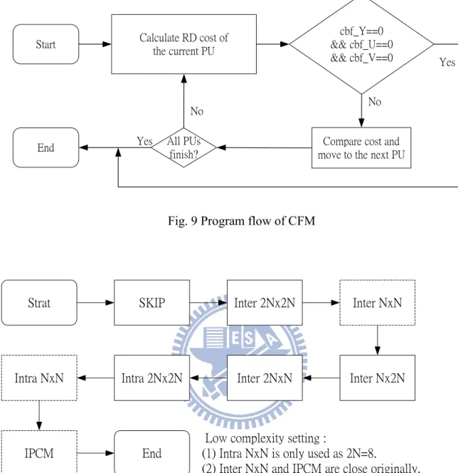
ECU and CFM are powerful tools for reducing complexity, but they are closed in the original settings of all configurations in HM5.0. An example of ECU is illustrated in Fig. 8, and the program flow of CFM with the execution order of PUs in the low-complexity profile is shown as Fig. 9 and Fig. 10 respectively.

Calculate RD cost of the current PU cbf_Y==0 && cbf_U==0 && cbf_V==0 Start

End All PUs

finish?

No No

Yes

Yes Compare cost and

move to the next PU

Fig. 9 Program flow of CFM

Strat SKIP Inter 2Nx2N Inter NxN

Inter Nx2N Inter 2NxN

Intra 2Nx2N Intra NxN

IPCM End

Low complexity setting :

(1) Intra NxN is only used as 2N=8.

(2) Inter NxN and IPCM are close originally.

Fig. 10 PU execution order in CU in the low-complexity setting

3.2

Analysis of Nested CU Quadtree Structure

The nested CU quadtree Structure decision process in HM5.0, which pursues the optimal structure selection, is described earlier in section 3.1.1. Although there exist FEN, ECU, CFM, and G-BFOS algorithms to reduce the encoding complexity, we like to further speed up the

and find out what factors producing the complexity.

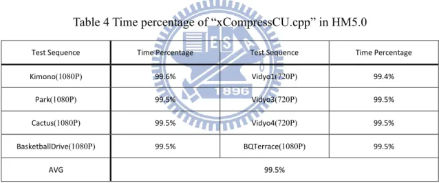
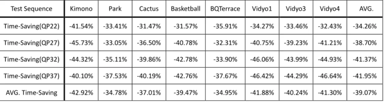
The HEVC encoder computes the R-D cost to select the best CU size, PU partition, and TU depth. The encoder spends a huge amount of computations on PUs and RQT in a CU quadtree to identify the lowest R-D cost. We measure the computing time of the function named “xCompressCU.cpp”, which is used for CU decision in HM5.0. In Table 4, we collect the execution time ratio of “xCompressCU.cpp” regarding the overall encoding time in 8 high-resolution test sequences for 16 frames, and the average time ratio is taken over 4 selected QP cases.

Table 4 Time percentage of “xCompressCU.cpp” in HM5.0

Test Sequence Time Percentage Test Sequence Time Percentage

Kimono(1080P) 99.6% Vidyo1(720P) 99.4%

Park(1080P) 99.5% Vidyo3(720P) 99.5%

Cactus(1080P) 99.5% Vidyo4(720P) 99.5%

BasketballDrive(1080P) 99.5% BQTerrace(1080P) 99.5%

AVG 99.5%

Table 4 shows a surprising result that CU decision takes more than 99% time in the low delay P with low complexity configuration. The computation associated with CU decision includes inter prediction, intra prediction, RQT, and calculate R-D cost, and we know that the computing time grows up rapidly with the increment of maximum admissible depth. Different maximum admission depth results in different compression efficiency and computational

complexity. In Table 5, we try the original block size setting of H.264/AVC with the maximum CU size equals 16 and the maximum admissible depth is 2 compared to the original setting in HEVC; that is, the encoder only uses 16 16 and 8 8 CUs to compress the video sequences with same testing condition as Table 4.

Table 5 Comparison of 64/4 CU structure and 16/2 CU structure (Maximum CU size / Maximum admissible depth)

Test Sequence Kimono Park Cactus Basketball BQTerrace Vidyo1 Vidyo3 Vidyo4 AVG. Time-Saving (QP22) -40.88% -43.75% -43.67% -42.95% -43.91% -45.39% -44.92% -44.40% -43.73% Time-Saving (QP27) -42.30% -46.01% -45.00% -44.56% -42.99% -45.57% -43.79% -45.22% -44.43% Time-Saving (QP32) -44.10% -45.33% -44.39% -45.46% -43.38% -44.47% -44.04% -44.40% -44.45% Time-Saving (QP37) -44.92% -45.08% -44.67% -46.15% -43.77% -43.99% -45.34% -43.14% -44.63% AVG. Time-Saving -43.05% -45.04% -44.43% -44.78% -43.51% -44.86% -44.52% -44.29% -44.31% Y BD-rate (%) 5.544 2.576 3.283 9.909 3.037 7.359 7.263 8.257 5.904 Y BD-PSNR (dB) -0.150 -0.078 -0.071 -0.167 -0.094 -0.207 -0.197 -0.193 -0.145

As depicted in Table 5, the 16/2 CU structure saves about 44% overall encoding time, but causes 5.9% luma BD-rate loss in average. In general, it is a trade-off issue between computational complexity and coding performance in designing a fast algorithm. Nevertheless, such a large loss from 16/2 CU structure is generally not considered cost-effective, so we are looking for other methods to accelerate the process of CU decision.

Chapter 4 Fast CU Size Decision Algorithm Design

In the following section, we first describe the problem and the target we want to achieve, and then we survey some ideas about fast CU quadtree decision algorithms, [20] and [21], published recently but not have been accepted in HM as the coding tools in our testing platform. After implementing the original platform, we measure and analyze its performance with many standard sequences, and propose some ideas referred from [21] to compensate the weakness of the testing platform.

4.1

Problem Formulation and Design Goal

Because HM5.0 has FEN, ECU, and CFM for CU fast algorithm, we try to design additional fast algorithms from different perspectives. The principle of our new tool should be different with those three existing tools, and the added tool should not reduce the performance of the existing and also be compatible with the CU quadtree structure in HM5.0.

For the above reasons and the simulation results in section 3.2, skipping the analysis of coding units in unnecessary depth is a possible way to accelerate encoding procedure, especially for the high resolution video. Typical fast algorithm performance or experimental results are examined by the ratio of time reduction, the bitrate and PSNR with the specified QP and R-D curve [20], [21]. Therefore, we set up a reasonable target of our final proposed

algorithm that reduces about 50% complexity and minimize the coding loss. Moreover, the collaborative effect between our proposed algorithm and the existent fast algorithms is also an important issue.

4.2

Related Work

Even though the original encoding procedure returns the best possible tree structure, its complexity is very high. Heuristics scene characteristics estimation is necessary to predict the optimal depth for the next encoded CU. In [20], the main idea is to accelerate the encoding procedure of HEVC by utilizing the correlation of related CUs. The encoder uses the size information of neighboring coding units and the processed depth-ratio in the previous frame to limit possible processed depth. In [21], a complexity-control method is proposed, which performs the time analysis and adjusts the number of fast encoding frames of each picture group. Recording the deepest depth used in the unit of LCU in the previous frame, the encoder finds the best possible tree structure until the recorded depth in each LCU in the current frame.

However, the methods, [20] and [21], are implemented in the earlier version HM, so we need to convert their ideas to fit our experimental platform HM5.0. Due to the above reasons and performance consideration, we remove the frame level algorithm in [20], and the time analysis in [21] is not suitable for our research because different computers would execute the

same program with different time, so we use QP value as the indicator to adjust our algorithm. The details will be described in the following sections.

4.3

Core Ideas of Fast CU Size Decision

The CU-level fast decision is based on the fact that the in the temporal and spatial neighborhoods, the motion and texture characteristics of a picture patch are similar. Therefore, we can predict the candidate CU depth by checking the size of its neighbor CUs (spatial) and co-located CU (temporal).

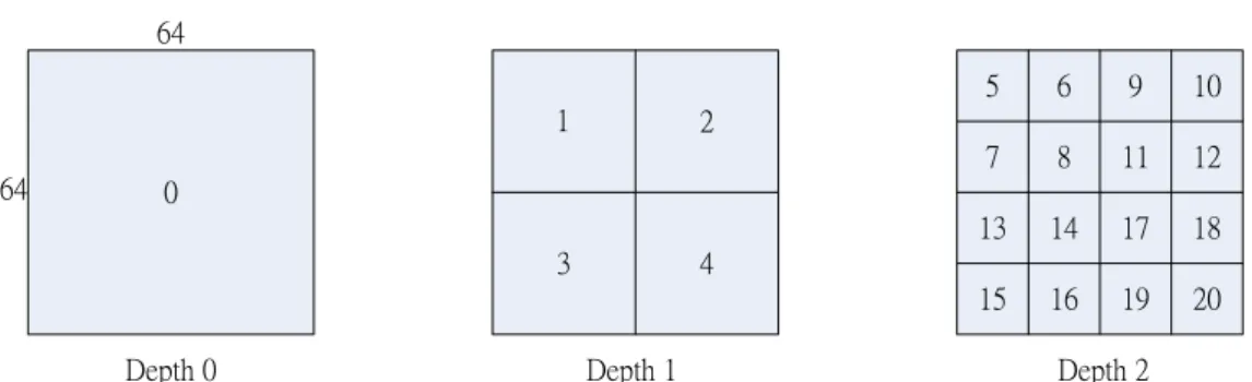
The data structure for HEVC is that each LCU includes 21 bits for representing the splitting information as illustrated in Fig. 11. The accuracy of the data structure extends to depth 2 which is sufficient for our fast decision. For example, during the encoding procedure, G-BFOS tells us that splitting the LCU into 4 sub-CUs is better due to its lower R-D cost. Then, the encoder will record the bit of index 0 in Fig.11 as 1 to indicate the splitting. Otherwise, the bit is set to 0.

0 3 2 7 4 5 6 9 10 20 8 11 12 13 14 17 18 15 16 19 1

Depth 0 Depth 1 Depth 2

64

64

The other important factor in our algorithm is the location of corresponding CUs. Fig. 12 depicts the relation between the referred neighboring CUs and the current encoded CU. The co-located CU means that the previous frame CU has the same position as the current encoded CU. It should be mentioned that our algorithm executes recursively in depth 0, depth 1, and depth 2 with the corresponding CU size of 2N2Nand CU index show in Fig. 11.

Fig. 12 Reference CUs and the current CU

As already stated in Chapter 3, some exceptions of losing reference CUs exist in Fig. 12 due to the encoding order or the picture boundary. When we want to encode a CU with index 4 in Fig.11, the right-top referenced CU has not been processed, so the encoder can’t find any information about the right-top CU as shown in Fig. 12. For this case, we ignore the right-top CU but still follow the decision rule that to be described in the next two sections. On the other hand, if the encoded CU is so close the boundary of picture that it loses more than one

4.3.1 Splitting Decision

The splitting decision is utilized for preventing the unnecessary prediction, RQT, and R-D calculation in a larger size CU. When the CU analysis begins at the current depth and all the following conditions are satisfied, the PU mode search in the current depth will be skipped except for the 2N N N / 2N inter modes, and then it jumps into the next depth directly. An example of splitting decision is illustrated in Fig. 13, where the current encoded CU in depth 0 chooses the splitting decision.

 The co-located CU has smaller CUs.  All neighboring CUs have smaller CUs.  The current encoding frame is not I frame.

Current Encoded CU Co-located CU 64 64

If all reference CUs prefer the splitting mode for lowering the R-D cost, which often implies that the region has complex residual texture, and the encoded block has a large probability in using the deeper depth to compress this CU. Nevertheless, when the depth of CU becomes smaller and smaller, we retain the inter modes,2N N N / 2N, with two MVs in the skipping data depth.

4.3.2 Termination Decision

The termination decision prevents the encoder from building a larger tree with a lot of computational complexity owing to the webs small CUs. If the encoder has already finished the CU mode decision in the current depth, the termination decision is determined by the following conditions. The mode decision whose depth is greater than the current depth will not be conducted when all the conditions are satisfied. Fig. 14 shows an example of termination decision, and the current encoded CU will not build any nodes with the depth larger than 0 in the CU quadtree. The termination decision often occurs in the smooth residual texture region or the static background.

 The co-located CU does not have any smaller CU.  3 or more neighboring CUs do not have any smaller CU.  The current encoding frame is not I frame.

Co-located CU Current Encoded CU 64 64

Fig. 14 An example of termination decision

4.3.3 Basic Fast CU Size Decision Scheme

Fig. 15 shows the flowchart of the basic fast CU size decision algorithm. It should be noted that the 2 fast decisions will not happen simultaneously in each depth of the encoded CU. From the above sections, we know that splitting decision and termination decision will not happen in I frame because a mismatched CU size in intra frame will result in a great PSNR drop or bit rate increase. Moreover, for the co-located CU and the consistence of reference CU size, we set up the experimental conditions for low delay P having only one reference frame (only one co-located CU) and the GOP size is equal to one to avoid the automatic increase in QP.

Start Set Depth=0 and CU address Depth<3 Splitting Decision Termination Decision Do mode decision in the current depth.

Compare the R-D cost by G-BFOS. Decide the best CU structure and

record it. Depth++ Back to (A) Do Inter modes Nx2N,2NxN. yes no yes no yes no no yes Tree complete? End (A) Set new depth

and CU address yes no Increase depth? Comparable for G-BFOS? yes no Set CU address

Fig. 15 Flowchart of basic fast CU size decision algorithm

4.4

Additional Tools

In this section, we try three methods to improve the performance of fast CU size decision. There is no BD-rate measurement in [20] and [21], so we check our luma BD-rate, BD-PSNR,

First, we observe that the coding loss increases as QP gets larger, such as 32 and 37. Nevertheless, the high QP setting is important for real-time application, and we should solve this problem. Secondly, the time-saving is small in the lower QP cases. We want to solve this problem because the encoder usually spends a lot of time compressing the videos at lower QP. In the following sub-sections, we analyze the data from the result of the proposed basic algorithm and design the modifications.

4.4.1 Frame Level Parameter Control

We collect the result of eight high-resolution video sequences with 32 frames per sequence, and find that the performance is better than that of 16/2 CU structure which is defined in section 3.2, but the coding loss is too high. Table 6 lists the BD-performance and time reduction ratio, and Fig.16 shows the R-D curve of sequence “Basketball”.

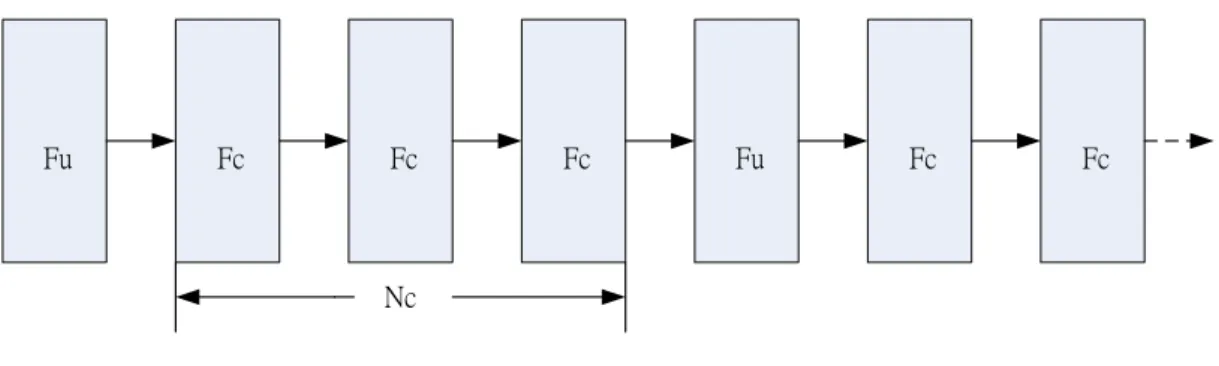
The reference curve is the original HM, and the test curve is our proposed method. We can find that two curves separate far in the higher QP cases, and we also notice that the time reduction ratio is very high, which may drop some necessary mode calculations. In [21], the depth-consideration fast algorithm sets the target of complexity from 40% to 100%, and there is a large amount of R-D performance drop between 40% and 60%. Therefore, we like to modify the method to maintain an appropriate complexity and to improve its BD-performance. The improved method in [21] defines two types of frames: the unconstrained frames (F_u) and

the constrained ones (F_c). F_c represents that the CU in the frame is encoded with the fast algorithm. On the contrary, the CU in F_u is processed in the original way to find the best CU quadtree structure. Each F_u is followed by a number of N_c constrained frames F_c as

illustrated by Fig. 17.

Table 6 Performance of the basic fast CU decision algorithm

Test Sequence Kimono Park Cactus Basketball BQTerrace Vidyo1 Vidyo3 Vidyo4 AVG. Time-Saving(QP22) -50.58% -37.73% -33.35% -35.83% -38.29% -41.56% -39.06% -40.78% -39.65% Time-Saving(QP27) -57.94% -41.80% -44.40% -51.38% -36.90% -51.74% -50.37% -53.91% -48.56% Time-Saving(QP32) -56.62% -46.10% -50.93% -55.60% -45.34% -60.38% -56.03% -60.28% -53.91% Time-Saving(QP37) -55.81% -53.26% -56.15% -61.44% -54.38% -65.85% -61.48% -67.31% -59.46% AVG. Time-Saving -55.24% -44.72% -46.21% -51.06% -43.73% -54.88% -51.74% -55.57% -50.39% Y BD-rate (%) 5.311 5.347 3.906 7.559 1.650 7.661 4.323 8.203 5.495 Y BD-PSNR (dB) -0.147 -0.160 -0.086 -0.127 -0.049 -0.200 -0.132 -0.181 -0.135 34 36 38 40 42 3.0 3.2 3.4 3.6 3.8 4.0 4.2 4.4 4.6 4.8 PSNR -dB Log10-bitrate-kbps BasketBall Reference Test

Fu Fc Fc Fc Fu Fc Fc

Nc

Fig. 17 Example of Nc=3

In Table 6, the BD performance drops due to the unlimited N_c. Our original proposed

algorithm sometimes takes the reconstructed frame with lower PSNR as the reference frame which results in inaccurate prediction. Therefore, we should pay attention to the PSNR loss with fixed N_c and set the tolerable bound for the PSNR decrease. The experiments set N_c

equal to 3, 6, 9, 12, and 15. Fig. 18 shows the suitable N_c as the intersection of two lines for

QP=22, 27, 32, and 37, where over 75% sequences limit their drops of PSNR under 0.1dB compared to the result of the original HM. The testing sequences and the frame number are the same as the stated in the beginning of this section.

We use the results from Fig. 18 to select the proper integral N_c for the corresponding QP. Then, we estimate the relationship between N_cand QP. The minimum square error

method is adopted for finding the approximated linear equation, which is

( 0.32 14.94), 46

    

c

N round QP QP (6)

c

N must be a positive integer, so we add the round operation outside the linear equation, and thus N_c is 0, when QP is larger than 46. The four QP values are taken into (6) iteratively to