Design and analysis of a dynamic scheduler for a flexible assembly system

(1)

Proceedings of the 1997 IEEE

Intemational Conference on Robotics and Automation Albuquerque, New Mexico - April 1997

Design and Analysis of a Dynamic Scheduler for

a

Flexible Assembly

System

Tz-Shian Huang

,

Li-Chen

Fu

,

and Yung-Yu Chen

Dept.

of Computer Science and Information Engineering

National Taiwan University, Taipei, Taiwan,

R.O.C.

Abstract

This paper proposes a rule-based dynamic scheduler for a flexible assembly system. We first introduce a flexible control system developed by Intelligent Robot and Automation Laboratory in National Taiwan Uni- versity. Based on that control system, the relationship between the control system and the scheduler is char- acterized. With focus on realization, hardware limi- tations such as long computation time and excessive memory-space usage are relaxed by incorporating several heuristic measures. The present work is applied t o the simulated robotized flexible assembly system in our laboratory.

1 Introduction

In

lieu

of

increasing complexity of assembly tasks and the desire for complete automation, integration of sensors, such as CCD cameras, force-torque sensor, optical switch and tactile sensor, into assembly work- stations and employment of AI techniques for solving problems become the natural resort. Thus, for

nowadays assembly process robots can become more intelligent and more capable of dealing with extremely difficult tasks. To date, there have been extensive re- search on applying knowledge-based approaches to the modeling of

a

robotic assembly cell, industrial applications, etc. [1, 21. Advantages of the above results in- clude good problem solving techniques and nice system architecture, but disadvantage also exists in requir- ing expert engineers t o extract knowledge from assembly jobs and assembly cell. The work by Huang and Lee [3] had also proposed a knowledge-based approach which assumes fixed assembly time. This resulting method with fixed assembly time assumption may be more suitable for the assembly tasks in a flow-line machine shop. For the sake of comparison, Noronha and Sarma [4] analyzed different knowledge-based approaches t o solve the scheduling problems. Then, they presented a taxonomy of planning and scheduling and integrated the AI approaches t o the knowledge rep ’- sentation. In this paper, we use a rule-based inference model t o solve the scheduling problem in the flexible control system. According to the assembly AND/OR graph and the configuration of the multi-robot assem-

bly system, the assembly rules can be generated sys- tematically. In this paper, IDA* search algorithm is applied to implement the inference engine. In order t o enhance the performance of the scheduler, several heuristics are adopted for the inference process.

Fu-

turemore, we propose and analyze several evaluation function for the flexible assembly system. Finally, we apply the flexible control system and the scheduling unit t o a real experimental two-robot assembly cell. This paper consists of six sections. Section 1 is an introduction of the concept of a robotized assembly system and of assembly scheduling. Section 2 describes a general control system for this robotic assembly environment and its scheduling unit. The problems to be solved are also defined in this section. Section 3 intro- duces a rule-based inference engine and describe how can it be used t o model the flexible assembly system. Section 4 describes how t o implement the inference engine by incorporating IDA* search. An experiment is provided in Section 5 t o demonstrate the flexibility and the enhanced performance of the inference engine. Finally, some conclusion are made in Section 6.

2 Robotized Flexible Assembly Sys-

tem

2.1 System Overview

A flexible assembly system (FAS) consists of a group of processing stations, interconnected by means of an automated material handling and storage system, and controlled by an integrated computer system. The ma-

jor advantage of the FAS over a traditional assembly line is flexibility. Some critical piece of equipment should be taken into consideration when configuring an assembly workstation, which includes robot, part loader, transfer mechanism, assembly fixture, sensor system, computer control system.

2.2 Flexible Control System -

EDAK

Jann [5] has proposed an object-oriented model for a control system architecture of robotic assembly automation, called event driven automation kernel (EDAK). There are four basic entities in the EDAK,

(2)

namely, Control Kernel, Application Task, Handler, Scheduler.

The system working scenario is that the event- detection handler informs the control kernel that some- thing just occurs, such as part's coming, assembly execution, etc., then the control kernel will update the system states and inform the system scheduler to make an optimal decision.

2.3 Scheduler for the Flexible Control

System

EDAK provides a convenient and uniform environment for the scheduler for an FAS. The assembly system scheduling problem can be described as follows: Given the following data: 1) System configuration, 2) The product assembly knowledge, the objective of the scheduler is to decide the "best" action for the system. The "best action" may be different for different crite- ria. In this paper, we minimize the total makespan

of

the final product assembly, or somewhat equivalently, the throughput rate.

The scheduler is

a

special handler of the control kernel, whereby all operations and decision makings can be made.

3 Rule-Based Modeling

of

Flexible

As-

sembly Systems

3.1 Rule-Based Inference System

The logistic view

of

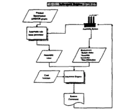
the scheduling process for an FAS is shown in Fig. 1. First, the modeling of an

as-

sembly system involves the transfer of the AND/OR graph and product assembly knowledge into the as- sembly rules for the assembly scheduling. Given the assembly rules and the state of the assembly system, the inference engine thus generates all of the possible assembly tasks, among which, its search algorithm will then search for the optimal ones.

Figure 1: The hierarchical view of the assembly scheduling for a n FAS.

D e f i n i t i o n 1 ( S t a t e )

A state is a predicate (or several predicates) which can describe a fact (or several facts). A state may has binding variable, i.e.,

a

variable whose attribute is yet to be determined, a n d will appear only in a production rule (abbrev. rule). A state is called a condition if it is in the precondition part of some rule.

D e f i n i t i o n 2 ( E n v i r o n m e n t )

An environment represents the whole

or

partial system information, which contain the following information: State list: A list of states altogether represent the status of all resource usage and the knowledge related to assembly sequences.

System time: The current time of the configuration to be registered.

Delayed state list: This is a list of two-tuple pails,

(T,S),

where

2'

is the delay time and

S

is the associated state, which means that the state

S

will be added into the state list of the environment right after time interval

T.

D e f i n i t i o n 3 ( R u l e )

A rule, R, is defined by a '/-tuple, i.e., R=(P, D, A, Delay, Action, Priority,

U),

where

P: a set of states that describe the precondition of the rule.

D:

delete-& a set of states that will be deleted from the system environment when the rule is executed.

A: addlist, a set of states that will be added to the environment after the rule is executed. Delay: the execution time of the rule, which may be modeled

as

a constant or a stochastic variable (uniform distribution, Gaussian distribution or any other probabilistic distribution).

Action:

an

external command that should be issued to the control system when the rule is fired.

Prioriry

E [l, n]: the firing priority, where n is the highest possible priority.

U:

unconditional rule, which will be fired in every constant

or

stochastic time interval.

D e f i n i t i o n 4 ( I n f e r e n c e E n g i n e )

Given a set of rules a n d an environment, an inference engine is a mechanism which will try to generate the best actions (commands) for a given environment by

the following steps:

1. The inference engine tries to find all enabled rules for the given environment.

(3)

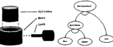
Figure 2: sentation.

A simple product and its AND/OR repre-

2. If the environment fails to match any rule precondition, the inference engine update the environment in the time frame until some unconditional rules are enabled

or

the updated environment will match the preconditions

of

some rules.

3.

If

both

of

the above fail, the inference engine will stop; otherwise, i t will choose the best rule from all the enabled rules for execution.

Remarks:

1. By updating the environment in the time frame, the inference engine will update t h e system time and remove the states that have the shortest delay time

T

from the delayed state list and add those into the state list of the environment. Up t o certain time instant, if this updated new environment enables any single rule, then the updating process will be interrupted by some state merging due t o a rule firing.

2. To choose the best rule out of all the enabled rules

for firing, the inference engine needs t o analyze the system state from the environment according to the so-called evaluation model and decide which rule is the best for the environment.

If

that is done, the states in the delete-part of the chosen rule are removed from the state list of the environment.

3.2 Modeling

of a

Robotized Flexible

As-

sembly System

3.2.1 Environment Representation

The state representation contains two main pieces of information, namely, the general environmental information and the assembly task information. The first one includes the information t o describe the assembly environment of a multi-robot assembly system, whereas the second one includes the information that expresses the desired product specification and the list of steps to complete the product assembly.

3.2.2 Assembly Rule Formation

In the following, we will demonstrate the formation of an assembly rule by using the product specification shown in Fig.

2.

Note that this product requires

Table 1 The rules for o p l and op2 in the AND/OR graph in Fig. 2.

RULE: ASSEMBLE BASE AND CYLINDER (opf) Precondition:

( Robot ?rid Ready )

( Robot ?rid Site ?sidl Base ?pidl ) ( Robot ?rid Site ?sid2 Cylinder ?pid2 )

( Robot ?rid Hand Empty ) ( Robot ?rid Ready )

( Robot ?rid Site ?sidl Base ?pidl ) ( Robot ?rid Site ?sid2 Cylinder ?pid2 ) ( Robot ?rid Ready )

( Robot ?rid Site ?sidl Basecylinder ?pidl ) Delete: Add: Action: Delay: Priority: 5 Unconditional: NULL

( Robot ?rid do-opl ?pidl ?pid2 ) ( Time Robot ?rid do-opl )

two types of assembly commands, o p l and op2. The AND/OR graph, indicates t h a t opl is the operation which assembles Cylinder and Base into the subassembly Basecylinder. To execute this operation, a free robot is needed first and then both of the aforemen- tioned parts are ready for assembly.

After the operation is started, we must delete some states t o indicate t h a t it is now in progress.

After the operation is done, the robot will produce one subassembly, Basecylinder, on site ?sidl and the robot, ?rid, will become ready again. The complete rules will be shown in Table 1.

4 Search-Based Dynamic Scheduler

4.1 Search-Based

Assembly

Dynamic

Scheduling

The objective of the inference engine is equivalent to finding the best rule for the current environment. The function of the inference engine can be decomposed into three, one is to find the enabled rules, another is t o choose the best rule from these enabled ones, and the other is to fire the rule. In the following, we describe how to apply search algorithm to the above problem.

4.1.1 IDA* Search Algorithm

The searching strategy in this paper is based on iterative-deepening

**A*,**

IDA

*

for short, search algo- rithm [6]. Iterative-deepening reduces the space com- plexity t o linear while preserving optimality. With an admissible heuristic estimate function (i.e., one that never overestimates), IDA* is guaranteed to find the optimal solution path. Moreover, it has been proved that IDA* obeys the same asymptotic branching factor

as A*, if the number of nodes grows exponentially with the solution depth [6]. This growth rate is called the

(4)

heuristic branching f a c t o r bh

.

The better space efficiency of IDA* is paid for an increased number of node expansions. On the average, IDA* requires bh/(bh - 1) times as many operations as A* [7].

4.1.2 M a t c h i n g Algorithm

Given an environment, the matching algorithm will find all enabled rules and the corresponding binding table for the rule from the rule database. Algorithm 1 and 2 below show the prototype of the rule-matching. A l g o r i t h m l : Matching Algorithm.

Input: Environment env.

Output: Find all enabled rules in the rule set and expand env. MAKECHILDNODE(env) (1) begin (2) (3) (4) ( 5 ) for priority p = n to 1

for each rule R choose priority = p

if (BINDING(env,R,BindingTableList)==OK) ExPANDRuLE(env,R,BindingTableList); (6) if(no enabled rules)

(7) UPDATETIME(enV); G o t o (2); (8) end

Algorithm2: Binding Algorithm. Input: Environment env, rule R. Ouput: ingTableList. BINDING(env,R,BindingTableList) (1) begin (2) (3)

Find all binding tables and store them into Bind-

for each BindingTable in the BindingTableList for each precondition p of rule R

Apply BindingTable to p.

if (p matches some state s in the state list of env) Resolve binding variable from p and then store it in BindingTable.

if p matches more than one state in the env

(4) ( 5 ) (6) (7) ( 8 ) (9) (10)

Resolve binding variable and add a new BindingTable in the list. e l s e return FAIL

return OK (11) end

4.2 Improve The Search Algorithm

Because IDA* algorithm does not retain path information from one iteration t o the next, the shallow tree parts are reexamined several times. There are several methods that improve the search performance by gath- ering information in the process

of

iterative-deepening. Here, we examine two type of strategies, node ordering heuristics and avoid re-expansion heuristics.

4.2.1 Node Ordering Heuristics

SORT

: This heuristic is based on rearrangement of the successors ni of the interior node n in decreasing order of their heuristic estimates h(n,). Succes- sors with high estimates, which means the node are closer t o the goal, are visited first. Although this scheme helps one in his search for optimal solutions, the savings achieved in (optimal) IDA* search rarely compensate for the increased overhead [8, p. 4711.

4.2.2 A v o i d Re-Expansion H e u r i s t i c s

Some researches discuss whether it is better to use graphs than t o use trees [9, lo]. In such cases, memory functions should be employed to avoid unnecessary re- expansions of previously visited nodes 1111.

CYCLE

: A moving cycle is a sequence of opera- tors, which after going through some intermedi- ate states from the starting state, finally returns to the starting state. Since iterative deepening maintains the current search path, moving cycles can be eliminated by comparing each newly generated node with those on the current path and pruning node that already appears on the path. TRANS : Move transpositions arise when different

paths end in the same node. They can be traced with a transposition table which stores every vis- ited node and the cost bound at which the posi- tion has been searched. When the current node is found in the table, its subtree can be pruned if the remaining cost bound is less or equal to the corresponding bound retrieved from the table. A good hashing function is required and must be designed case by case. The size of the transposition table should be allocated as large as possible. Reinefeld and Marsland have shown that this heuristic can reduce the search node visited by IDA* in [12].

4.3 Evaluation Function for Flexible

As-

sembly System

Many off-line scheduling problems usually assume that the system is deterministic and the performance measure is the total makespan. However, for an on-line scheduler, to minimize the total makespan is difficult. In this paper, the objective of the scheduler is to minimize the production time for every product assembly, or, somewhat equivalently, the throughput rate.

We first define productive operation and nonpro-

ductive operation. The definition of productive op-

eration is the operation which will change a part or

produce a new part. In an assembly system, "ASSEM- BLE", "SCREW" are all productive operations, whereas "MOVE", "PICK" and "PUT" are nonproductive opera-

tions.

Now we define g(env) as the time spent from the root environment to the current environment, and h(env) as the estimated time required to produce some final product.

For every final product assembly, find the estimated time t o finish the assembly of the product. The value

of h ( e n v ) will be the smallest value of the estimated

time.

STEP

1 : For every product, find all parts required for

STEP 2 : Perceive that these parts in Step 1 are all sitting in the assembly sites of a n available robot, it.

(5)

and then calculate the total time required to finish the assembly of the product. Because all parts are in the robot sites, all operations required are

productive ones. We call this time period as pro-

ductive operation t i m e , Tp.

STEP

3 : In practice, there are usually some parts required for the final product which are currently not ready yet. They can be either fed from the part loading machine or obtained from the buffer. Thus, for any part which is not yet in the robot site, we add one estimated operation time,

Testimate, which is the smallest time elapse for the

robot t o get the part from buffer, conveyor belt, or other sites. If there are

n

parts required to finish the product which are not currently ready in the robot sites, then the total nonproductive

operation t i m e ,

Tnp

=

n

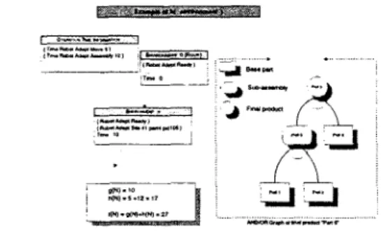
' Testimate.

For example, consider a simple assembly cell which contains only one robot. This cell is t o produce the product, denoted as part5, whose AND/OR assembly graph is shown in Figure 3. Assume now the robot's site contains one part, part3. In this example, the robot is unable to produce part5 because of lack of part 4. Assume that the next part loading will load part4 into the cell, which normally takes

5

seconds. Further, assume the operation time is 12 seconds for the robot. Thus, h(end) = 5

+

12 = 17 seconds and f ( e m ) = 10

+

17 = 27 seconds.

Theorem 1 T h e evaluation function, h(env), defined

above is admissible. -

Proof:

According to the above definition, the estimated time t o the goal

for

a given environment is

as

follows:

h(env) = Min(Tp,

+

Tnpi

I

For every product i) Comparing h(env) with the real operation time T* required to reach the goal for the given env, we can find that Tp = Tpf and Tnp

5

T;p, where T; and T;p represent the real productive operation t i m e and the real nonproductive operation t i m e required to oal respectively. Thus, the estimate function, h ( e n 8 is

admissible.

A

cost function is said t o be monotonic if the cost of a child is always greater than or equal t o that of its parent. Korf prove that, with a monotonic cost function, iterative-deepening search expands nodes in the best-first order [13, p.451.

Theorem 2 T h e cost f u n c t i o n , f ( e n v ) , defined above is monotonic.

The proof is shown in appendix.

* . . .

--

-

Figure 3: An example of the estimate function, h(env).

I Y J

Figure 4: System layout

5 Experiment and Analysis

We are going t o demonstrate an example solved by the proposed inference engine and dynamic scheduler. The example is the scheduling problem for an experimental robotized flexible assembly system in our laboratory.

The system is two-robot assembly cell which is ded- icated t o assembling various types of mechanical parts serially sent in through a conveyor belt.

All the parts are sent into the cell through a conveyor belt in a serial order, and are on-line identified using an overhead camera and a side camera. Both robots are identical in terms of their assembly function, i.e., each of them can perform any type of assembly task. Buffers are assumed t o be present in order t o store the parts which already arrived but are not yet ready to be assembled. The whole system is controlled by EDAK. The equipment structure is shown in Fig. 4.

5.1 Experimental Result

The experiment is a multi-robot simulation based on the software environment called CimStation

runs

on a Sun-Sparc 10 workstation. The algorithm of each function unit in simulation is written in SIL which is a robotic simulation language, while the assembly scheduling programs are written by C++ language. In the simulation, both robots have four assembly sites. The average time for generating each schedule is about

2-10 seconds.

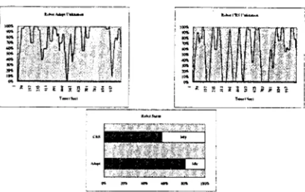
The average number and maximum of buffer usage are 6.322 and 10 respectively. The utilization of each robot, Adept and CRS, are shown in Figure 5

.

(6)

Figure 5: Utilization of robot Adept and CRS.

6 Conclusion

This paper is an extension of [14]. The relationship between the scheduler and t h e

EDAK

is discussed in Section 2.

The result of the improved

IDA*

algorithm in Sec- tion 4.2 is consistent with t h e research by Reine- feld [12].

It

is noteworthy t h a t the most time

con-

suming part is t h e matching procedure. The improved matching procedure in Section 4.2 is similar to RETE [15]. Efficiency arises from its exploitation of temporal redundancy in working memory and struc- tural similarity among productions.

Appendix

The cost function, f(env), defined in section 4.3 is mono-

tonic. Proof:

For all nodes n‘ and n, where n‘ is a child of n,

f

(n) = 9 ( 4

+

h(n)

f(n‘) = g(n’)

+

h(n’)

The firing rule between node n and n‘ may be one of the following kind of rule.

1. Control rule: No actual command is issued. In this case, the environment time will not change. Thus, g(n) = g(n’) and h(n) = h(n’). So that, 2. Productive operation: If the operation takes time

Top,

then g(n’) = g ( n )

+

Top

and h(n’) =

h(n) -Top. Thus,

f(d)

= f(n).

3. Nonproductive operation: Assume the operation takes time To?. Thus, g(n’) = g ( n )

+

Top, but there are two possible cases for the estimate function:

(a) If this operation takes one primitive part re- quired for the product assembly, the estimated time to reach the goal will be decreased by

T e a t i m a t e , i.e., h(n’) = h ( n ) - T e a t i m a t e , because

one new part is now in the robot site. Because Testimate

I

Top, we have f(n’)

L

f(n).

(b) Otherwise, h(n’)

2

h(n), and thus f(n’)

2 f

(4.

Consequently, the cost function, f ( e n v ) , is monotonic.

f ( n ) =

!(.’I.

References

[I] M. S. Fox and S. F. Smith, “ISIS - a knowledge-based system for factory scheduling,” Expert System, vol. 1, no. 1, pp. 22-49, 1984.

[2] H. V. Brussel, F. Cottrez, and P. Valckenaers, “SES- FAC: a scheduling expert system for flexible as- sembly cells,” in Proceedings of 1990 IEEE confer-

ence o n Robotics and Automation, (Cincinnati, Ohio),

[3] Y . F. Huang and C. S. G. Lee, “A frame work of knowledge-based assembly planning,” Proceedings of

1991 I E E E conference o n Robotics and Automation,

vol. 2, pp. 599-604, Apr. 1991.

(41 S. J. Noronha and V’. V. S. Sarma, ‘‘Knowledgy; based approaches for scheduling problems: a survey,

I E E E Bansaction on Knowledge and Data Engineer-

ing, vol. 3, pp. 160-171, June 1991.

[5] C.-S. Jann, “Flexible control system for robot assembly automation,” Master’s thesis, National Taiwan University, Department of Computer Science and In- formation Engineering, 1994..

[6] R. E. Korf, “Depth-first iterative-deepening: An op- timal admissible tree search,” Artificial Intelligence, vel. 27, no. 1, pp. 97-109, 1985.

[7] M. E. Stickel and W. M. Tyson, “An analysis of con- secutively depth-first search with applications in au- tomated deduction,” in Proceeding 9th International

Joint Conference o n Artificial Intelligence, pp. 1073-

1075, 1985.

[8] C. Powley and R. E. Korf, ‘Single-agent parallel win- dow search,” IEEE Transaction on Pattern Analysis

and Machine Intelligence, vol. 13, pp. 466-477, May

1991.

[9] R. Ramaswamy and A. K. Sen, “Single machine scheduling as a graph search problem with path- dependent arc costs,” in Proceedings ECAI-92, Europ.

Conference Artificial Intelligence, (Vienna), pp. 1-5,

Aug. 1992.

[lo] A. Mahanti, S. Ghosh, D. S. Nau, A. K. Pal, and L. Kanal, “Performance of IDA* on trees andjjraphs,” in Proceeding 10th National Conference on rtzficial

Intelligence, AAAI-92, pp. 539-544, 1992.

[ll] J. C. Pemberton and R. E. Korf, “Incremental path planning on graphs with cycles,” in Proceedings of the

1st International Conference on Artificial Intelligence

PIanning Systems, (College Park, MD, USA), pp. 179-

188, Morgan Kaufmann Pub1 Inc, June 1992. [12] A. Reinefeld and T. A;, Marsland, “Enhanced

iterative-deepening search, I E E E Transaction on

Pattern Analysis and Machine Intelligence, vol. 16,

pp. 701-710, July 1994.

[13] R. E. Korf, “Linear-space best-first search,” Artificial

Intelligence, vol. 62, pp. 41-78, 1993.

[14] H.-H. Hsu, “Fully automated robot assembly cell: scheduling and simulation,” Master’s thesis, National Taiwan University, Department of Computer Science and Information Engineering, 1994.

[15] C. L. Forgy and S . J. Shepard, “Rete, a fast match algorithm,” A I Ezpert, pp. 34-40, Jan. 1987. pp. 1950-1955, 1990.