暫存資訊在即時屏幕空間全域照明技術之應用

全文

(1)國立交通大學多媒體工程研究所碩士論文. 暫存資訊在即時屏幕空間全域照明技術之應用 Real-Time Screen Space Global Illumination with Cached Information. 研究生：林祐生指導教授：施仁忠教授. 中華民國一百零二年七月.

(2) 暫存資訊在即時屏幕空間全域照明技術之應用 Real-Time Screen Space Global Illumination with Cached Information 研究生 : 林祐生. Student : Yu-Sheng Lin. 指導教授 : 施仁忠教授. Advisor: Prof. Zen-Chung Shih. 國立交通大學多媒體工程研究所碩士論文. A Thesis Submitted to Institute of Multimedia Engineering College of Computer Science National Chiao Tung University in partial Fulfillment of the requirements for the Degree of Master in Computer Science. July 2013 Hsinchu, Taiwan, Republic of China. 中華民國一百零二年七月.

(3) 暫存資訊在即時屏幕空間全域照明技術之應用. 研究生: 林祐生. 指導教授: 施仁忠教授. 國立交通大學多媒體工程研究所. 摘. 要. 模擬全域照明現象在電腦圖學的領域中，一直是火熱的研究議題。漫射相互反射、焦散、折射和軟陰影等現象提供了重要的視覺線索，並且它們的加入可大幅地改善圖像的真實感，而為了做更多的即時應用，像是電腦遊戲或虛擬實境系統，能即時的計算全域照明現象是很重要的。. 本篇論文結合反射陰影圖(Reflective Shadow Maps)、螢幕空間環境遮蔽(Screen Space Ambient Occlusion)及百分比漸進濾波(Percentage Closer Filtering)等方式繪製出逼真的場景，並藉由改變取樣模式和累積前一張畫面的資訊提高圖像品質，最後利用反向重投影法(Reverse Re-projection)使得收斂好的畫面在鏡頭移動的過程中盡可能地重複利用，達到效能提升，經由實作證明本演算法在大型的場景下也有不錯的表現。. I.

(4) Real-Time Screen Space Global Illumination with Cached Information Student: Yu-Sheng Lin. Advisor: Prof. Zen-Chung Shih. Institute of Multimedia Engineering National Chiao Tung University. ABSTRACT Simulating global illumination has been the intense research topic in computer graphics for many years. Effects such as diffuse inter-reflection, caustics, refractions and soft shadows provide the important visual cues that help the viewer to understand spatial relationships and also drastically improve the realism of a rendered scene. Thus, in order to do many real-time applications like computer games and virtual reality systems, computing global illumination at interactive frame rates is significant. In this thesis, we propose an algorithm combining reflective shadow maps, screen space ambient occlusion and percentage closer filtering for realistic image synthesis. By changing sampling patterns and accumulating the results of previous frames, we can improve the quality. Finally, in order to achieve high performance, we exploit reverse re-projection technique to reuse converged information while the camera is moving. We demonstrate that the algorithm works well for large-scale scenes at interactive frame rates.. II.

(5) Acknowledgement. First of all, I would like to express my sincere gratitude to my advisor, Prof. Zen-Chung Shih for his guidance and patience. Without his encouragement, I would not complete this thesis. Also thank to Prof. Yu-Ting Tsai and all the members in Computer Graphics and Virtual Reality Laboratory for their reinforcement and suggestion. Thanks for those people who have supported me during these days. Finally, I want to dedicate the achievement of this work to my family and the natural beauty around daily life.. III.

(6) Contents 摘. 要....................................…………………….………………………………I. ABSTRACT..........................………………………………………………………….II Acknowledgement...............………………………………………………………….III Contents........………………….…………………………………………………….IV List of Figures........……………………………………………..………………..…VI List of Tables................................................................................................................IX Chapter 1 Introduction..................….........………………………………...…...…...1 1.1 Motivation……………...…......……………………………….…………...1 1.2 System Overview……………………………………………………………3 1.3 Thesis Organization………………………………………………………….4 Chapter 2 Related Work..............……………..……..………………………………...5 2.1 Ambient Occlusion…………..……………………….……...……….…...5 2.2 VPL Methods..................................…………………...………………..…..6 2.3 Temporal Coherence Methods in Rendering……………………..…....…...7 Chapter 3 Algorithm.............………………………...........……………….......…….9 3.1 Temporal Coherence……………………...…………………………………10 3.1.1 Reverse Re-projection Cache …………………………………..10 3.1.2 Accumulation with Confidence Value …………………………..12 3.2 Ambient Occlusion………………….……………..…….……………..15 3.2.1 SSAO Generation ……………………………………………..16 3.2.2. Exploiting Cached Information …………………...………………..19. 3.3 Indirect Illumination…….…………………….……………………..21 3.3.1. Reflective Shadow Maps……………….……………………21 IV.

(7) 3.3.2. Exploiting Cached Information…………….……………..……25. 3.4 Fake Soft Shadow………………………………………….………………..27 3.4.1. Exploiting Cached Information …………………...………………..28. Chapter 4 Implementation and Results...................................…….............…........…29 Chapter 5 Conclusion and Future Work.............................…...….........…….........…43 References........……………………….........…….........……………………....…….44. V.

(8) List of Figures Figure 1.1: Banding artifacts and noise artifacts.................................................….......3 Figure 1.2: Overview of workflow....………………………………………………….3 Figure 2.1: Disk-shaped elements and Grayish flat surfaces.........................................6 Figure 3.1: Invisible pixels are shown in red...............................................................11 Figure 3.2: Images with banding artifacts, noise artifacts and Gaussian filter...........12 Figure 3.3: The flowchart of amortized sampling........................................................14 Figure 3.4: The sampling method of Mittring [7]........................................................15 Figure 3.5: The drawbacks from the SSAO algorithm of Mittring [7]........................16 Figure 3.6: The world-space positions and world-space normal vectors in G-buffer.......................................................................................................... 17 Figure 3.7: The observation of ambient occlusion.......................................................17 Figure 3.8: (a) The initial sampling directions. (b)Random vector texture for perturbing the sampling pattern per pixel. (c) The more contribution of ambient occlusion will always be close…..........…………………………………..................18 Figure 3.9:. (a) Before blurring. (b) After blurring....................................................19. Figure 3.10: (a) SSAO without accumulating cached information. (b) SSAO with accumulating cached information….......................................................................20 Figure 3.11: Surface point p is illuminated by actual light source and reflected light source.………………………………………………………………………………..21 Figure 3.12: From left to right: world space positions, world space normal vectors, depth information, and reflected radiant flux……………………………………….22 Figure 3.13: (a) Project the pixel p into RSMs for gathering the VPLs. (b) The visualization of the sampling pattern…………………………………………………23 VI.

(9) Figure 3.14: The results of elephant scene with and without visibility test……….24 Figure 3.15: The results of room scene with and without visibility test………..25 Figure 3.16: Direct illumination with indirect illumination. From left to right: Indirect illumination with 512 and 1024 VPLs…………………………………….26 Figure 3.17: The comparison of indirect illumination with and without cached information………………………………………………………………………26 Figure 3.18: The Percentage Closer Filtering method……………..……………....27 Figure 3.19: Hard shadows (left).The soft shadows are created by using 49 samples (middle).The soft shadow are created by using only 9 samples and with accumulating cached data (right)……………………………………………………………….28 Figure 3.20: The shadows with and without using cache information……………..28 Figure 4.1: The discarded pixels must be complete computed………………...…29 Figure 4.2: SSAO with 32 samples. The left image does not use the tiled update strategy. The right image uses the tiled update strategy……………………31 Figure 4.3: Indirect illumination with 512 VPLs. The left image does not the use tiled update strategy. The right image uses the tiled update strategy…………..…31 Figure 4.4: The shading results are discontinuous on the borders of the refreshed regions………………………………………………………………………………..31 Figure 4.5: The SSAO of Mittring [7] on Buddha & Box scene and Dragon & Box scene. The comparison with and without cached information………………………33 Figure 4.6: The comparison of our SSAO with and without cached information……34 Figure 4.7: The comparison of RSMs with and without cached information……35 Figure 4.8: The comparison of shadows with and without cached information….…36 Figure 4.9: The four difference scenes using our approach………………………….37. VII.

(10) Figure 4.10: There are more pixels have to be recomputed in the more complex scene........................................................................................................42. VIII.

(11) List of Tables Table 4.1: The comparison of the performance from Figure 4.9………………38 Table 4.2: The comparison of the performance for the Sponza scene…………39 Table 4.3: The comparison of the performance for the Sibenik scene…………40 Table 4.4: The comparison of the performance for the Conference Room scene……41. IX.

(12) Chapter 1 Introduction 1.1 Motivation In order to create realistic scenes, only local illumination is not enough. Global illumination provides visual cues to synthesize photorealistic images, effects such as diffuse inter-reflections, caustics, refractions and soft shadows are examples of it. Unfortunately, they are complex light interactions with a huge computational cost. Recently, with the rapidly increasing computation power of graphics hardware, global illumination has become visible to render scenes in real time.. Nowadays, only indirect illumination in real-time is sufficient in games. But for the complex and large scenes, it’s still the major challenge. Fortunately, image-space global illumination which uses deferred shading process decouples the scene geometry and prevents the execution of shading for hidden surfaces. Shadow is also an important element for enhancing realism in computer graphics. In recent years, many real time shadow algorithms are proposed both for hard and soft shadows.. In this thesis, we consider not only one-bounce indirect illumination but also ambient occlusion for increasing the realism without performing costly visibility computation. We use the Reflective Shadow Maps (RSMs) [3] which can efficiently create virtual point lights (VPLs) for the single-bounce diffuse indirect lighting and present the simple screen space ambient occlusion (SSAO) algorithm which was sparked by 1.

(13) Mittring et al. [7] and Bavoil et al. [2] . Furthermore, we use the Percentage Closer Filtering (PCF) [10] for generating anti-aliased shadows. In order to create the soft shadows, we refine the original percentage closer filtering technique by accumulating the cached shadow values with their confidence values.. To reduce the banding and noise artifacts due to a low number of samples and varying sampling patterns on each visible surface point as show in Figure 1.1, we change the sampling patterns each frame and accumulate the required information per pixel over time by using a so-called history cache in screen space.. Finally, in order to achieve significant performance, we apply a simple method called reverse re-projection caching. The basic idea was independently proposed by Scherzer et al. [12] and Nehab et al. [8]. There are some limitations in our method. The light source and the objects of the scene must be static. If they are moving, we have to re-compute each frame. The main contributions of this thesis include: 1. Combine the idea of reusing information from previous frames with the expensive calculation of global illumination. 2. To omit spatial filtering that is typically necessary for noise and to resolve banding artifacts, we accumulate the cached data by using a special confidence value for updating history cache. 3. Our algorithm is based on the deferred shading pipeline so we avoid the expensive calculation of global illumination for hidden surfaces. 4. Combining reflective shadow maps, screen space ambient occlusion and percentage closer filtering for realistic image synthesis.. 2.

(14) Figure 1.1 Banding artifacts (left), noise artifacts (right). 1.2 System Overview. Figure 1.2 Overview of our proposed system. (Based on the deferred shading pipeline) 3.

(15) Our system is a multi-pass rendering algorithm running on the GPU. Figure 1.2 shows an overview of our rendering architecture. First, we generate textures that are called G-buffer (see Figure 1.2 (a)) and reflective shadow maps (see Figure 1.2 (b)). They store the information from the view of the camera and the light source respectively. Furthermore, we cache the information per pixel at time step t-1 (see Figure 1.2 (d)). Second, we always detect cached data whether the camera moves or not by using the world positions of camera view (see Figure 1.2 (c)). If an occlusion is detected (marked red in Figure 1.2 (c), left), we have to re-compute current results (see Figure 1.2(e)) and combine them to get the final image (see Figure 1.2(f)). Otherwise, we check the previous data in history cache which are converged or not (see Figure 1.2(i)). Third, when the required information in history cache is converged, we can reuse and combine them with the current direct lighting result (see Figure 1.2(h)). On the other hand, we render the current scene geometry by changing the sampling patterns and accumulating it with previous data (see Figure 1.2(g)).. 1.3 Thesis Organization This thesis is structured as follows: First we review the related work about screen space ambient occlusion, VPLs based global illumination and temporal coherence techniques in Chapter 2. In Section 3.1, we explain why we can get the converged results while taking into account changing the sampling patterns and using confidence value to accumulate the data between current and past frame. Then, we depict how to combine the idea of exploiting Temporal Coherence with the generations of screen space global illumination (e.g., SSAO, RSMs) in Section 3.2 and Section 3.3. We show that using the cached shadow values for rendering anti-aliased shadows and soft shadows in Section 3.4. Chapter 4 provides our implementation and the results. Conclusion and future work are discussed in Chapter 5. 4.

(16) Chapter 2 Related Works In this chapter, we review some related works of ambient occlusion and VPL based methods. Then, we briefly survey various applications that exploit temporal coherence.. 2.1 Ambient Occlusion Ambient occlusion (AO) is a shading technique for approximating global illumination that was originally developed by Landis [6]. Shadowing of ambient light is referred to as ambient occlusion. It gives perceptual clues of curvature and enhances the geometry features of the scene. Unfortunately, computing the ambient occlusion requires casting a large number of rays on each surface point. This is too expensive for real-time applications. Therefore, Bunnell [1] computes the ambient occlusion by using disk-based occluders as show in Figure 2.1 (a) and produces high quality results. However, it has a huge pre-processing step for dynamic objects, and the per-vertex occlusion algorithm reveals a linear interpolation artifact. Crytek [7] first developed a screen space ambient occlusion approach used in the PC game Crysis. It sparsely samples visibility rays against the scene depth buffer and produces plausible results. The main drawback of this method is the incorrect gray flat surfaces as shown in Figure 2.1 (b). Shanmugam and Arikan [15] describe an approach splitting the ambient occlusion problem into high and low frequency part. One uses an image-space method on near objects. The other generates coarse AO using spherical proxies on distant occluder. The results of their algorithm are quite well, but 5.

(17) performance is bad due to the two separate computation parts. Bavoil et al. [2] proposed Image-Space Horizon-Based Ambient Occlusion which computes AO by comparing the horizon angles between sampled point and surface point. It works more effectively and yields nice results.. Figure 2.1 (a) Disk-shaped elements, Bunnell [1] (b) Grayish flat surfaces. 2.2 VPL Methods Standard global illumination methods such as path tracing, radiosity and photon mapping can give full and accurate global illumination. But the algorithms require minutes or hours to render a realistic scene. Keller [5] introduced Instant Radiosity which can approximate the indirect illumination of a scene by using a set of virtual point lights (VPLs). This method is popular because it produces no noise images and drastically reduces the computational cost. However, it is expensive to trace the light path for determining a set of VPLs as well as calculate visibility by creating an individual shadow map for each VPL. Consequently, In order to resolve these problems, many VPL based methods are developed. Dachsbacher and Stamminger [3] extend a standard shadow map to a reflective shadow map storing the lighting information. All pixels of a shadow map are considered as indirect light sources. This 6.

(18) novel idea efficiently addresses the production of virtual point lights and offers the approximating indirect illumination at interactive frame rates. In addition, to account for indirect shadows, Ritschel et al. [11] use a crude point-based representation of geometry to accelerate the shadow map generation for each VPL. Yang et al. [16] construct the per-pixel linked lists to implement real-time indirect shadows on the GPU. But their method requires large memory to store all the fragments of the scene objects. Dong et al. [4] cluster the VPLs into a small number of virtual area lights (VALs), hence the number of the shadow maps can be decreased. The above methods have demonstrated that accurate visibility between VPLs and surface points is not necessary for indirect illumination because human visual is slightly sensitivity to the correctness of indirect shadows.. Although the above screen space global illumination algorithms (e.g., Mittring[7], Dachsbacher and Stamminger[3] ) have several advantages such as computation not depending on scene complexity, avoidance of the execution for hidden surfaces and simple implementation, there are a lot of potential for quality and speed improvements by exploiting temporal coherence. In the following section, we briefly introduce a variety of applications using the concept of temporal coherence in rendering.. 2.3 Temporal Coherence Methods in Rendering Temporal coherence (TC) describes the correlation or the predictable relationship of contents between adjacent moments in time. It has been around for computer graphics. By taking advantage of it, the computation of the rendering tasks is alleviated and the quality of the images is improved. For example, in general, there 7.

(19) are very little difference in the shading computation between two consecutive frames. Therefore, re-computing everything each frame is wasteful. The key to utilizing TC is how the previous computed information are stored and reused. Scherzer et al. [12] and Nehab et al. [8] independently proposed a technique called Reverse Re-projection Cache . The idea is to store the previous shading results in a screen buffer and project the current pixel to the prior frame. By comparing the stored depth with current depth, it can decide whether the pixel was visible in the past frame (detail in section 3.1). This special framework has been used for a variety of rendering applications, like anti-aliased hard shadows [8,12] , real-time soft shadows [13,14] , motion blur and stereoscopic rendering [8]. Our approach is inspired by their concept of reusing data and spreading the computation over several frames.. In summary, our algorithm uses the reflective shadow maps to simulate one bounce indirect illumination and the screen space ambient occlusion to enhance the realistic of the scene. By taking up the idea of reverse re-projection cache, we can save redundant re-calculation and provide the high quality images.. 8.

(20) Chapter 3 Algorithm In this thesis, we propose a novel idea of reusing cached information of previously rendered frames to enhance the screen space global illumination algorithms such as Reflective Shadow Maps [3] and standard screen space ambient occlusion [7]. In addition, our algorithm is based on deferred shading pipeline. By taking advantages of temporal coherence, we display the high quality images which consider single bounce indirect illumination, ambient occlusion and soft shadows in real time.. 1. In section 3.1, we describe in detail how to implement reverse re-projection cache [8,12] for getting the available data stored in history cache and how to accumulate the cached information by taking into account the confidence of these information. 2. In section 3.2, we depict the simple implementation of screen space ambient occlusion and exploit the idea of temporal coherence to generate no noise solution without smoothing filter. 3. In section 3.3, we briefly introduce the Reflective Shadow Maps [3] to compute indirect illumination and focus specifically on how to use the cached information to improve the quality of the indirect illumination produced by RSMs technique. 4. In section 3.4, we also show that we can combine Percentage Closer Filtering [10] with our caching strategy to increase the shadow accuracy and to render the fake soft shadows. 9.

(21) 3.1 Temporal Coherence Various rendering applications exploit temporal coherence to achieve high quality images at a lower cost. When using temporal coherence, there are two important decisions. One is how the previously computed data are stored. The other is how the stored data are efficiently retrieved. As long as we resolve these problems, we can obtain the benefit from temporal coherence.. 3.1.1 Reverse Re-projection Cache In order to reuse available information, we follow the reverse re-projection cache [8,12]. We first define a buffer called history cache similar to Nehab et al. [8] and Scherzer et al. [12]. This buffer is viewport-sized and stores the required information at visible surface points in previous frame. Fortunately, on modern graphics hardware, we can represent the buffer as the textures as shown in Figure 1.2 (d) and store it in the texture memory. Therefore, history cache is efficiently maintained on the GPU. In addition, we require some necessary data for determining whether the current pixel was visible in the earlier frame. Unlike Nehab et al. [8] and Scherzer et al. [12] store the non-linear depth for the new and the old frame in the buffer, we store the world-space positions in the history cache and do the re-projection in fragment shader. Formally, let 𝑊𝑡 denote the world-space position of the pixel stored in G-buffer at time step t as shown in Figure 1.2 (a). Let 𝑃𝑡−1 and 𝑉𝑡−1 symbolize the projection matrix and the view matrix at time step t-1. Consequently, for static geometry, we can do the following transformation to get the clip-space coordinates 𝐶𝑡−1 at time step t-1: 𝐶𝑡−1. =. 𝑃𝑡−1 ∗ 𝑉𝑡−1 ∗ 𝑊𝑡 10. (1).

(22) Then we do the perspective division to get the normalized device coordinates 𝑁𝑡−1 . In order to get the correct texture coordinates 𝑡𝑒𝑥 𝑡−1 , we should scale the 𝑁𝑡−1 to the range [0, 1]. Here, we define 𝐻𝑡 (𝑡𝑒𝑥𝑡 ) as the buffer values of the texel at time step t. Therefore, we can get the correspondent world-space position at time step t-1 stored in the history cache : 𝑊𝑡−1 = 𝐻𝑡−1 (𝑡𝑒𝑥𝑡−1). (2). Finally, we have to detect dis-occlusions for deciding whether the pixel at time step t was visible at time step t-1. Accordingly, we compute the Euclidean distance between 𝑊𝑡 and 𝑊𝑡−1 and compare it with a threshold 𝜀 : ‖𝑊𝑡 − 𝑊𝑡−1 ‖ ≤ 𝜀. (3). If the distance is greater than a threshold, the pixel was not presented in the last frame, and there are no previous data can be safely reused. Note that the lower the threshold is, the more invisible pixels appear (see Figure 3.1 ).. Figure 3.1: Invisible pixel is shown in red. The left image is before a translation, and the middle image is after a translation to left with 𝜀= 0.1. The right image is after a translation to left with 𝜀=0.01. The more invisible pixels will impact the performance.. 11.

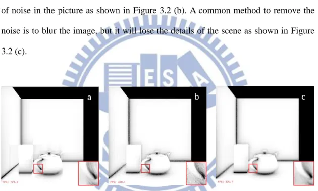
(23) 3.1.2 Accumulation with Confidence Value In spite of avoiding the execution on the hidden surfaces, the screen space global illumination techniques still have some bottlenecks in their sampling strategy (e.g., Mittring [7] ; Dachsbacher and Stamminger [3] ). For example, in order to increase the frame rates, they usually reduce the number of samples. Thus, it brings the banding artifact as shown in Figure 3.2 (a). The general way to alleviate this artifact is using the various sampling pattern at each pixel. But it also introduces a lot of noise in the picture as shown in Figure 3.2 (b). A common method to remove the noise is to blur the image, but it will lose the details of the scene as shown in Figure 3.2 (c).. b. a. c. Figure 3.2: (a) SSAO with a single sampling pattern. (b) SSAO with the various sampling patterns. (c) SSAO with Gaussian filter.. The simple way to remove the above drawbacks is using a lot of samples, but it is too expensive for interactive applications. Fortunately, since we can efficiently get the previous data by using the reverse re-projection technique shown in Section 3.1.1. We may use these cached information well for improving the quality of the image. Consequently, our goal is spreading the cost of sampling. We first rotate a sampling pattern which has a small number of samples and jitter the sampled positions to generate slightly different result stored in history cache of each frame. Secondly, by 12.

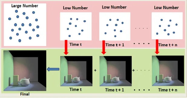
(24) recursively accumulating the results, we can get the high quality image. The key is how to accumulate the cached information. Therefore, we take the confidence of the previous solution into account, which can be motivated as follows. The various sampling patterns may capture the difference information. We can estimate how confident the value from previous frame is by calculating the difference between the cached result at time step t-1 and the current result as follows :. 𝑐𝑜𝑛𝑓𝑖𝑑𝑒𝑛𝑐𝑒 =. 1 −. 𝑠𝑎𝑡𝑢𝑟𝑎𝑡𝑒( ‖𝑉𝑡−1 − 𝑉𝑡 ‖ ) 1+𝑏𝑖𝑎𝑠. (4). Where 𝑉𝑡−1 is the per-pixel value which is obtained by reverse re-projection technique, and saturate means clamping the specified value within the range of 0 to 1. The value of bias is user-specified for avoiding zero condition of the confidence and adjusted to your applications to achieve the quality you want. In the other words, this confidence value tells us how much information the cached result did not have. While we complement the difference over several frames, we would forecast the final result without variance. Thus, we apply the following operation:. 𝑉𝑝 = (𝑐𝑜𝑛𝑓𝑖𝑑𝑒𝑛𝑐𝑒)𝑉𝑡−1 + (1 − 𝑐𝑜𝑛𝑓𝑖𝑑𝑒𝑛𝑐𝑒)𝑉𝑡. (5). We take the confidence value to be a weighting factor for estimating how much percentage of the value between two consecutive frames we can take, and 𝑉𝑝 means the predicted value. Note that because of taking the confidence value per pixel to be a weighting factor, we can avoid spending time to find the acceptable value for the weight. Figure 3.3 depicts the flowchart of our amortized sampling method.. 13.

(25) Figure 3.3: The top row shows various sampling patterns in each frame. The bottom row shows the correspondent results.. 14.

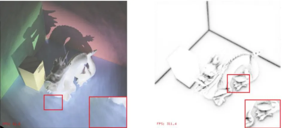
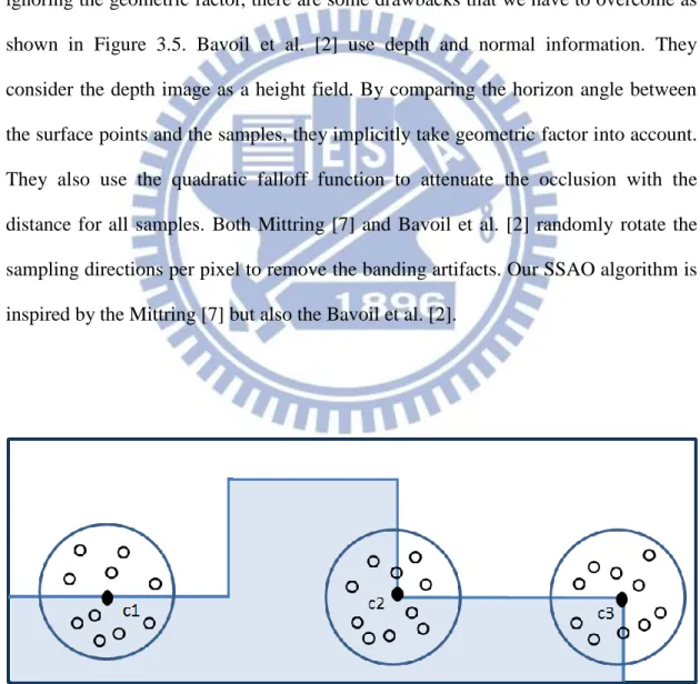
(26) 3.2. Ambient Occlusion Ambient Occlusion (AO) is a popular method for approximating global. illumination. It gives perceptual clues of depth and curvature, and it also enhances the geometry features of the scene. For economic reason, we need simpler implementation and higher performance. Therefore, Screen Space Ambient Occlusion (SSAO) was published by Mittring [7]. This algorithm uses only depth information and samples the 3D space around visible point c as shown in Figure 3.4. Because of ignoring the geometric factor, there are some drawbacks that we have to overcome as shown in Figure 3.5. Bavoil et al. [2] use depth and normal information. They consider the depth image as a height field. By comparing the horizon angle between the surface points and the samples, they implicitly take geometric factor into account. They also use the quadratic falloff function to attenuate the occlusion with the distance for all samples. Both Mittring [7] and Bavoil et al. [2] randomly rotate the sampling directions per pixel to remove the banding artifacts. Our SSAO algorithm is inspired by the Mittring [7] but also the Bavoil et al. [2].. Figure 3.4: Half of the samples are inside the wall and half outside (left). Three quarters of the samples are inside the wall (middle). A quarter of the samples are inside the wall (right). 15.

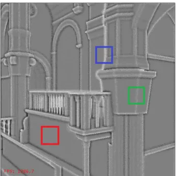
(27) Figure 3.5: The flat surfaces are gray color (red block).The edges appear brighter (green block).The white halos are around the edges of the objects (blue block).. 3.2.1 SSAO Generation We first need the two world-space information taken from eye’s G-buffer. One is world-space positions, and the other is world-space normal vectors as shown in Figure 3.6. Moreover, we can observe the following condition. For every visible point p, if the sampled point q on the occluding surface is close to it, there are fewer photons around it as shown in Figure 3.7. We also have to add the attenuation parameter which is important to avoid common SSAO artifact on the border of an object. Consequently, the ambient occlusion AO at a point p with a surface normal 𝑛⃗ is :. AO(𝑝, 𝑛⃗) =. 1 𝑘. ∑𝑘𝑖=1. ⃗⃗⃗ ∙ ⃗⃗⃗⃗⃗⃗⃗ max(𝑛 𝑝𝑞𝑖 ,0) D(𝑑). D(𝑑) = 1.0 + a𝑑 + b𝑑 2. (6). (7). 16.

(28) Where 𝑞𝑖 means the i-th sample around the surface point p, D denotes the attenuation function, constant 1.0 is used to avoid singularity and then 𝑑 is the distance between 𝑞𝑖 and p. Besides, a and b are user-specified parameters to control the effect of the attenuation with distance.. Figure 3.6: The world-space positions in G-buffer (left). The worldspace normal vectors in G-buffer (right).. Figure 3.7: The sample q does not occlude the surface point p, because the dot product of the surface normal and the vector 𝑝𝑞 ⃗⃗⃗⃗ is zero in case (a). The surface point p is occluded, because the dot product is not zero in case (b).. 17.

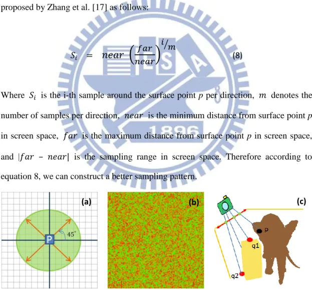
(29) In order to achieve higher performance, we limit the number of samples and use the regular sampling directions per pixel as shown in Figure 3.8 (a). Furthermore, in order to avoid the banding artifact, we should perturb the sampling pattern per pixel in screen space by using a random 2D-vectors texture that discards the z component as shown in Figure 3.8 (b). In general, we can say that the samples that are close to the surface point p in world space are also close in the screen space and contribute more occlusion to surface point p as shown in Figure 3.8 (c). Consequently, according to the above reasons, we apply the technique that is used to partition the view frustum proposed by Zhang et al. [17] as follows:. 𝑆𝑖. = 𝑛𝑒𝑎𝑟. (. 𝑖⁄ 𝑚. 𝑓𝑎𝑟 𝑛𝑒𝑎𝑟. ). (8). Where 𝑆𝑖 is the i-th sample around the surface point p per direction, 𝑚 denotes the number of samples per direction, 𝑛𝑒𝑎𝑟 is the minimum distance from surface point p in screen space, 𝑓𝑎𝑟 is the maximum distance from surface point p in screen space, and |𝑓𝑎𝑟 – 𝑛𝑒𝑎𝑟| is the sampling range in screen space. Therefore according to equation 8, we can construct a better sampling pattern.. (a). (b). (c). Figure 3.8: Our initial sampling directions (a). Random vector texture for perturbing the sampling pattern per pixel (b). the sample q1 is close to surface point p in world space as well as in screen space. Otherwise, q2 is far from surface point p in world space as well as in screen space (c). 18.

(30) Finally, we have to blur the image for reducing the noise as another image-space ambient occlusion technique as shown in Figure 3.9. However, the operation of blurring should impact the performance. In Section 3.2.2 we show that we can use the cached information to remove this redundancy.. Figure 3.9: Before blurring, there is a lot of noise in left image. After blurring, the details of the objects are lost in right image.. 3.2.2 Exploiting Cached Information In order to get better results of screen space ambient occlusion, we require a lot of samples that is an unwise choice for real-time applications. Therefore, we can take up the idea of amortizing the cost of sampling (In section 3.1.2). First, we use the reverse re-projection technique (In Section 3.1.1) to get the past value of ambient occlusion 𝐴𝑂𝑡−1. Second, before perturbing the sampling pattern per pixel, we rotate the sampling directions with fixed angle 𝜃 and slightly scale the sampling range. We then compute the current ambient occlusion 𝐴𝑂𝑡 . Third, we calculate the difference between past and current ambient occlusion according to Eq. 4. Finally, we use Eq. 5 to accumulate 𝐴𝑂𝑡−1 and 𝐴𝑂𝑡 by taking the difference value for weighting factor. Note that we should specify the value to limit the number of times to 19.

(31) rotate the sampling pattern. Therefore, we can avoid the unlimited accumulation and determine whether the results are already converged or not. In our implementation, 𝜃 is ten degrees. Figure 3.10 shows the comparison of SSAO with and without employing cached information.. Figure 3.10: Both left and right SSAO use 32 samples per pixel. In the left image, SSAO without accumulating cached information has the noisy artifacts. In the right image, SSAO with accumulating cached information provides less noisy artifacts and maintains the details of the objects.. 20.

(32) 3.3. Indirect Illumination Consider Figure 3.11, both direct and indirect illumination are shown. Indirect. illumination can increase the scene luminance for improving the image quality. Unfortunately, the computational cost of it is too expensive for real-time applications. However, in general case, we can only consider one-bounce indirect illumination. Reflective Shadow Maps [3] is a technique for efficiently generating one-bounce indirect illumination. In the following, we describe how to implement Reflective Shadow Maps and how to refine the results of it by taking the cached information into account.. Figure 3.11: Surface point p is illuminated by actual light source (marked green arrow).Surface point q is illuminated by reflected light source (marked red arrow).. 3.3.1 Reflective Shadow Maps Reflective Shadow Maps (RSMs) [3] is a virtual point light (VPL) based method. It uses the observation that all one-bounce indirect illumination is caused by surfaces that are directly illuminated from the actual light source. Therefore, each pixel in the shadow map can be considered as a VPL that illuminates the scene. We need to extend a standard shadow map by storing more lighting information such as world space positions, world space normal vectors, depth and reflected radiant flux as shown in 21.

(33) Figure 3.12. We then use the following equation to calculate the contribution of a VPL q at a surface point p.. 𝐼𝑝 = Φ𝑞. D =. max(0 , 𝑁𝑝 ∙𝐷)max(0, 𝑁𝑞 ∙(−𝐷)) ‖𝑞−𝑝‖2. 𝑞−𝑝 ‖𝑞−𝑝‖. (9). (10). Where 𝐼𝑝 denotes the irradiance at a surface point p, 𝑁𝑝 is a normal vector of p, 𝑁𝑞 is a normal vector of VPL q, Φ𝑞 is the radiant flux of q and D represents a unit vector between p and q.. Figure 3.12: From left to right: world space positions, world space normal vectors, depth information, and reflected radiant flux.. This question depicts how can we gather the VPLs to compute indirect illumination. As the standard shadow mapping, we can project the pixel p stored in G-buffer into the reflective shadow maps and do the sampling to gather the VPLs as shown in Figure 3.13 (a). The original RSMs uses a fixed sampling pattern which can be generated by simple random sampling or Poisson Disk sampling. Figure 3.13 (b) 22.

(34) shows our sampling pattern. Note that we multiply the samples with their squared distance because of the varying sampling density.. (a). (b). Figure 3.13: Project the pixel p into RSMs for gathering the VPLs (a). The visualization of the sampling pattern (b).. Since original RSMs ignores the occlusion for the indirect light sources, in some special cases it may lead to severe wrong results. To approximate visibilities of VPLs, we can use the world space positions and depth information stored in G-buffer and RSMs. Like [7] that samples visibility rays against the scene depth buffer, we first get the unit vector D between the surface point p and VPL q according to Eq.10. Next, we do the same sampling strategy according to Eq. 8 along the direction of vector D. Let 𝑠𝑖 is the i-th tested sample and 𝑍𝑡 (𝑠𝑖 ) represents the depth value of the sample 𝑠𝑖 in eyes space. Finally, as the standard shadow mapping, we can determine whether the VPL q contributes the radiance on p or not by comparing the depth value 𝑍𝑡 and 𝑍𝐺 which is the corresponding depth value stored in G-buffer. If 𝑍𝑡 > 𝑍𝐺 , the VPL q should be rejected, and the visibility weighting factor V(𝑞) is zero. By multiplying Eq. 9 and weighting factor V(𝑞) together, we can obtain the enhanced results that have better visual perception as shown in Figure 3.14 and Figure 3.15. Note that this method is not the correct calculation of visibility, and it should introduce the performance overhead. In our experiments, it approximately halves the frame rate. 23.

(35) Figure 3.14: Top row: The view of light source (left). The view of camera (right). Note that the green points are VPLs which provide too much radiance toward the floor point (marked orange) and red points are tested samples. Bottom row: The rendered scene without the visibility test (left). The rendered scene with the visibility test (right).. 24.

(36) Figure 3.15: The middle wall is not present in the view of the light source. There are severe light-bleeding artifacts without the visibility test for VPLs (left). The light-bleeding artifacts disappear with the visibility test for VPLs (right). 3.3.2. Exploiting Cached Information. Since the computational cost of indirect illumination is very expensive, we need to limit the number of VPL samples. In our experiments, the number of samples that is no more than 512 is suitable for real-time applications. However, if the samples are few, the banding artifacts will appear as shown in Figure 3.16. Fortunately, we can remove this disgusting artifact by accumulating the cached information. First, we get the past value of one-bounce indirect illumination 𝐼𝑡−1 by using reverse re-projection. Next, we always have to rotate the sampling pattern to generate the current indirect illumination 𝐼𝑡 . We then calculate the difference between 𝐼𝑡−1 and 𝐼𝑡 as Eq. 4. Finally, we follow the Eq. 5 to combine 𝐼𝑡−1 with 𝐼𝑡 . Therefore, we can get the final converged results. Figure 3.17 shows the comparison of indirect illumination with and without accumulating the cached information.. 25.

(37) Figure 3.16: Direct illumination with indirect illumination. From left to right: Indirect illumination with 512 and 1024 VPLs. The left image is darker than the right image and the banding artifacts in the left image are more apparent than the right image.. Figure 3.17: The comparison of indirect illumination with 512 VPLs. The banding artifacts are apparent without accumulating cached information (left). The result is smooth by accumulating cached information (right).. 26.

(38) 3.4. Fake Soft Shadow Shadow is an important effect for realistic image synthesis. Nowadays,. shadow mapping which creates the shadows by comparing the depth of the pixels in eye’s view with the corresponding depth value in the shadow map is a popular real-time algorithm for dynamic hard shadows. Unfortunately, it always suffers the perspective aliasing and the projective aliasing problems that influence the visual perception in the images. A feasible solution is using Percentage Closer Filtering [10] (PCF). This technique takes more than one sample around each shaded point to compare their depths, and averages the results of their comparisons to get the anti-aliased shadows as shown in Figure 3.18. In general case, we can extend this technique to obtain the soft shadows by taking no less than 49 samples. However, it still leads to a slightly banding artifact. Fortunately, we can use the cached shadow values to improve the quality of the shadows as previous work does [8]. We not only rotate but also scale the sampling pattern to generate slightly different shadows. We then take the different values of them as the weighting factors to accumulate the shadow values.. Figure 3.18: We can get the results of depth comparisons between a surface point p and the samples around it in shadow map. An average of the values stored in the mask can be an occlusion rate to create the anti-aliased shadows. 27.

(39) 3.4.1 Exploiting Cached Information We first take the past shadow value 𝑆𝑡−1 per pixel from history cache. Before computing the new shadow value 𝑆𝑡 per pixel, we have to rotate the sampling pattern and scale the size of pattern each frame. Afterwards, we can get the difference between them according to Eq. 4. By taking the difference value as weighting factor, we can avoid spending time to find the acceptable value for the weight that is used to accumulate the shadow values 𝑆𝑡−1 and 𝑆𝑡 . Figure 3.19 and Figure 3.20 show the comparisons.. Figure 3.19: Hard shadows (left).The soft shadows are created by using 49 samples (middle).The soft shadows are created by using only 9 samples and the cached data (right).. Figure 3.20: The shadows of left image without accumulating cached information have apparent aliasing than the shadows of right image with accumulating cached information. ( Both images use 49 samples.). 28.

(40) Chapter 4 Implementation and Results We implement our approach by using OpenGL 4.3 with OpenGL Shading Language. In order to avoid multiple rendering passes for the generation of G-buffer and RSMs, we use multiple render targets (MRT).. To increase the rendering performance of indirect illumination, we take the advantage of low-frequency nature of diffuse lighting as original RSMs [3] does. Therefore, we first compute the low-resolution indirect illumination. We use a half of full resolution that is the best trade-off between high performance and high quality in our experiments. We then get the interpolated full resolution indirect illumination by testing the four surrounding low-resolution samples each pixel . If the sample’s world space normal and world space position close to the pixel’s normal and position, we can compute the contribution of each sample by using bilinear interpolation. Otherwise, the discarded samples are computed later in the final gathering pass. Figure 4.1 shows the discarded samples.. Figure 4.1: The red pixels are discarded samples and must be completely computed.. 29.

(41) In order to achieve high frame rate, we can reuse the converged results from SSAO, one-bounce indirect illumination and soft shadows by caching them in the buffer. Note that we still have to refresh them after a few frames. Because when the camera and the light source are moving, the shading condition is changed. Furthermore, when doing the reverse re-projection to get the cached information, it always gradually accumulates the reconstruction error. This problem is caused by resampling the discrete data. The one to one pixel mapping is difficult. The common solution is doing bilinear interpolation which is directly supported by the modern graphics hardware. Unfortunately, if we keep reusing cached results over several frames, the bilinear interpolation will lead to over blurred results. Therefore, we follow a refresh strategy described in Nehab et al. [9]. We can divide the screen into a grid of 𝑛 tiles, and randomly select a non-repeated tile to be updated. Figure 4.2 and Figure 4.3 show the comparison with and without using the tiled update strategy. Note that the size of a tile will influence the performance and the quality. In our experiment, the region of a tile in SSAO implementation is 64×64 pixels. The region of a tile in one-bounce indirect illumination is 16× 16 pixels and the region of a tile in shadow implementation is 64×64 pixels. On the other hand, we found that the shading results are discontinuous on the borders of the refreshed regions as shown in Figure 4.4. Fortunately, they are not too obvious to influence the visual perception of the results. In addition, in our experiment, we found that there is not a remarkable performance speedup for the PCF soft shadows, because the calculation of PCF is not complex. It only needs doing the depth comparison. Nevertheless, we still can take the advantage of temporal coherence to improve the shadow quality.. 30.

(42) Figure 4.2: SSAO with 32 samples. The left image does not use the tiled update strategy. The right image uses the tiled update strategy.. Figure 4.3: Indirect illumination with 512 VPLs. The left image does not the use tiled update strategy. The right image uses the tiled update strategy.. Figure 4.4: The shading results are discontinuous on the borders of the refreshed regions. 31.

(43) The results of our algorithm are implemented on a desktop PC with Intel Core i7 930 CPU 2.8GHz, 8G RAM, and NVIDIA GeForce GTX 480 video card. All images are rendered at a resolution of 512×512, and the tested scenes are static. We compute one-bounce indirect illumination with 512 VPLs on a half resolution and interpolate the solution into the full resolution image. All the results of our SSAO are rendered with 32 samples.. We also implement the SSAO method of Mittring [7] by accumulating the cached information of SSAO. Then we compare it with the results using Gaussian blur as shown in Figure 4.5. Figure 4.6 compares our proposed SSAO method that uses the cached information with the results using Gaussian blur. Figure 4.7 shows the indirect illumination results that are combined with direct illumination, and we compare them with the results using the cached information. Figure 4.8 shows the pseudo soft shadows that are computed by using the PCF technique with 49 samples, and we compare them with the results that use the cached information to improve the quality. Figure 4.9 shows the final converged results that are composed of ambient occlusion, one-bounce indirect illumination and direct illumination. Table 4.1 shows the average timings of the results from Figure 4.9 with and without reusing past information. Tables 4.2~4.4 show the converged results of large scenes and the frame rates for their scene walkthroughs with and without using cached information of previous frames.. 32.

(44) (a). 16 samples/pixel. (d). 16 samples/pixel. (b). 16 samples/pixel + blur. (e). 16 samples/pixel + blur. (c). 16 samples/pixel + cached data. (f). 16 samples/pixel + cached data. Figure 4.5: Left column: Buddha & Box scene. Right column: Dragon & Box scene. Note that the over blurred results are in (b) and (e), and the finer converged results are in (c) and (f). Our approach also works well for the SSAO technique proposed by Mittring [7]. 33.

(45) (a). 32 samples/pixel. (d). 32 samples/pixel. (b). 32 samples/pixel + blur. (e). 32 samples/pixel + blur. (c). 32 samples/pixel + cached data. (f). 32 samples/pixel + cached data. Figure 4.6: Left column: Buddha & Box scene. Right column: Dragon & Box scene. Note that the over blurred results are in (b) and (e), and the finer converged results are in (c) and (f). Our approach works well on both scenes.. 34.

(46) (a). 512 VPLs/pixel. (d). 512 VPLs/pixel + cached data. (b). 512 VPLs/pixel. (e). 512 VPLs/pixel + cached data. (c). 512 VPLs/pixel. (f). 512 VPLs/pixel + cached data. Figure 4.7: Left column: No use cached information. Right column: Use cached information. The images of right column have less banding artifacts than left column. 35.

(47) (a). Hard shadows. (d). Hard shadows. (b). 49 samples/pixel. (e). 49 samples/pixel. (c). 49 samples/pixel + cached data. (f). 49 samples/pixel + cached data. Figure 4.8: Left column: Buddha & Box scene. Right column: Sponza scene. The hard shadows have aliasing artifacts in (a) and (d). The smooth shadows are produced by the PCF technique in (b) and (e). The high-quality soft shadows are produced by using the PCF technique and the cached shadow values in (c) and (f).. 36.

(48) (a). Direct lighting. (b). Direct lighting + SSAO. (c). Direct lighting + SSAO +Indirect lighting. (d). Zoom in. Figure 4.9: The four difference scenes from top row to bottom row. All images are computed by using our approach. Column (a) to (c) display different effects such as pseudo soft shadows , ambient occlusion and one-bounce indirect illumination. 37.

(49) Table 4.1 shows the experimental results of our approach. We compare the difference in performance for various scenes from Figure 4.9 with and without reusing past information stored in history cache. All the scenes have the same camera path for their walkthroughs. We measure the average timings of SSAO, one-bounce indirect lighting and the final combined results. The results of SSAO without using cached information have the annoying noise artifacts. We apply the Gaussian 5×5 blur to remove them. It only takes approximately 0.5 millisecond. Note that we re-compute the G-buffer of camera view for each frame. The results taking the advantages of temporal coherence have not only the high quality but also the great performance.. SSAO Scene. Reuse data Blur Yes/No. Y/N. Venus (43,357 faces). Yes. N. No. Dragon (6,514 faces). One-bounce. SSAO + Indirect. Indirect lighting lighting + direct lighting. fps. VPLs. fps. Total fps. 206. 512. 51. 46. Y. 170. 512. 34. 31. Yes. N. 426. 512. 73. 63. No. Y. 280. 512. 43. 38. Bunny (69,451 faces). Yes. N. 147. 512. 46. 41. No. Y. 130. 512. 32. 28. Buddha. Yes. N. 102. 512. 34. 31. (100,000 faces). No. Y. 89. 512. 26. 23. Table 4.1: The comparison of the performance for different scenes with and without reusing past data.. 38.

(50) Dabrovic Sponza (66,450 faces). Direct illumination. SSAO. Indirect illumination. Direct and Indirect illumination + SSAO. Table 4.2: Characteristic walkthroughs for the Sponza scene. The performance of the scene rendered by using cached information is mostly better than the results that do not use cached information. 39.

(51) Sibenik (75,284 faces). Direct illumination. SSAO. Indirect illumination. Direct and Indirect illumination + SSAO. Table 4.3: Characteristic walkthroughs for the Sibenik scene. The performance of the scene rendered by using cached information is mostly better than the results that do not use cached information. 40.

(52) Conference Room (331,179 faces). Direct illumination. SSAO. Indirect illumination. Direct and Indirect illumination + SSAO. Table 4.4: Characteristic walkthroughs for the conference room. The performance of the scene rendered by using cached information is mostly better than the results that do not use cached information. 41.

(53) Tables 4.2~4.4 show that our approach also works well for large-scale scenes. Note that there are more pixels have to be recomputed in the more complex scene when the camera moves as shown in Figure 4.10.. Figure 4.10: A simple scene is composed of a dragon and a box (left). A complex scene is the conference room (right). There are more pixels (marked red) in the right image have to be recomputed than in the left image when the camera moves left.. 42.

(54) Chapter 5 Conclusion and Future Work In this thesis, we propose a novel approach that utilizes temporal coherence to enhance the screen space global illumination algorithms such as reflective shadow maps and screen space ambient occlusion. We demonstrate that both the quality and the performance can be improved by reusing the previous results. In addition, our algorithm is easy to implement. However, we only can handle one-bounce diffuse indirect lighting and the light source must be static.. In the future, we want to extend our algorithm to handle the dynamic scenes. For example, whenever an object moves, the effects of global illumination on this object and the effects of global illumination caused by it have been changed. Therefore, how to efficiently know where the regions of the screen have to be recomputed is a difficult problem. Even though we can create a movement mask by rasterizing the bounding volumes of the moving objects, it still not absolutely resolves the problem. One of the reasons is that if the scene object is big, its projection might cover a large portion in the movement mask and more pixels have to be updated. The other is that we should know where the pixels in screen are influenced by the moving objects. Finally, we find that the over blurred results occur since we reuse the cached results over many frames. Consequently, we would investigate that how to keep the better accuracy of the reused results.. 43.

(55) References [1] Bunnell, M. 2005 Dynamic Ambient Occlusion and Indirect Lighting. In GPU Gems2, M. Pharr, Ed. Addison Wesley, Mar., ch. 2, 223-233. [2] Bavoil, L., Sainz, M., and Dimitrov, R. 2008. Image-space horizon-based ambient occlusion. In SIGGRAPH '08: ACM SIGGRAPH talks, ACM, New York, NY, USA, 1-1. [3] Dachsbacher, C., and Stamminger, M. 2005. Reflective Shadow Maps. In Proceedings of the ACM SIGGRAPH 2005 symposium on Interactive 3D Graphics and Games, 203-213. [4] Dong, Z., Grosch, T.,. Ritschel, T., Kautz, J., and Seidel, H.-P.. Real-time. indirect illumination with clustered visibility. In Proceedings of Vision, Modeling, and Visualization Workshop, 2009. [5] Keller, A. 1997. Instant Radiostiy. In SIGGRAPH '97, 49-56. [6] Landis, H. 2002. Production-ready global illumination. Course notes for SIGGRAPH 2002 Course 16, RenderMan in Production. [7] Mittring M.: Finding next gen: Cryengine 2. In SIGGRAPH 07: ACM SIGGRAPH 2007 courses, ACM, pp. 97-121. [8] Nehab, D., Sander, P.V., and Isidoro, J.R.: The real-time reprojection cache. In ACM SIGGRAPH 2006 Sketches, ACM Press, p. 185. [9] Nehab, D., Sander, P.V., Lawrence, J., Tatarchuk, N., Isidoro, J.R.: Accelerating real-time shading with reverse reprojection caching. In: Graphics Hardware. (2007), p. 25-35. [10] Reeves, W. T., Salesin, D. H., and Cook, R. L. 1987. Rendering antialiased shadows with depth maps. In Computer Graphics (Proceedings of SIGGRAPH '87), vol. 21, 283-291. [11] Ritschel, T., Grosch, T., Kim, M. H., Seidel, H.-P., Dachsbacher, C., and Kautz, J. 2008. Imperfect shadow maps for efficient computation of indirect illumination. ACM Trans. Graph. (Proc. SIGGRAPH Asia) 27, 5, 12:1-129:8. 44.

(56) [12] Scherzer, D., Jeschke, S., Wimmer, M.: Pixel-correct shadow maps with temporal reprojection and shadow test confidence. In Kautz, J., Pattanaik, S., eds.: Rendering Techniques 2007 (Proceedings Eurographics Symposium on Rendering), p. 45-50. [13] Scherzer, D., Schw ̈ rzler, M., Mattausch, O., and Wimmer, M. 2009. Real-Time Soft Shadows Using Temporal Coherence. In Advances in Visual Computing: 5th International Symposium on Visual Computing (ISVC 2009), Springer, Lecture Notes in Computer Science, 13–24. [14] Schw ̈ rzler, M., Luksch, C., Scherzer, D., and Wimmer, M. 2013. Fast Percentage Closer Soft Shadows using Temporal Coherence. In Proceedings of ACM Symposium on Interactive 3D Graphics and Games 2013, pages 79-86. [15] Shanmugam, P., and Arikan, O. 2007. Hardware Accelerated Ambient Occlusion Techniques on GPUs. In Proceedings of ACM Symposium in Interactive 3D Graphics and Games. ACM, B. Gooch and P.-P.J. Sloan, Eds., 73-80. [16] Yang, J.C., Hensley, J., Grün, H., and Thibieroz, N.: Real-Time Concurrent Linked List Construction on the GPU. Comput. Graph. Forum 29(4): 1297-1304 (2010) [17] Zhang, F., Sun, H., Xu, L., and Lun, L. K. 2006. Parallel-Split shadow maps for large-scale virtual environments. In VRCIA ’06: Proceedings of the 2006 ACM International Conference on Virtual Reality Continuum and its Applications, ACM,New York, NY, USA, 311–318. 45.

(57)