邊界切割方法在車牌辨識系統之應用

國 立 交 通 大 學

電 機 與 控 制 工 程 學 系

碩 士 論 文

邊界切割法在車牌辨識系統之應用

A New Edge Segmentation Method Applied to the

License Plate Recognition System

研 究 生：侯 宜 穎

指導教授：陳 永 平 教授

邊界切割法在車牌辨識系統之應用

A New Edge Segmentation Method Applied to the

License Plate Recognition System

研 究 生：侯 宜 穎

Student：Yi-Ying Hou

指導教授：陳永平 博士 Advisor：Dr. Yon-Ping Chen

國 立 交 通 大 學

電機與控制工程學系

碩士論文

A Thesis

Submitted to Department of Electrical and Control Engineering

College of Electrical and Computer Engineering

National Chiao Tung University

In Partial Fulfillment of the Requirements

For the degree of Master

In

Electrical and Control Engineering

June 2006

Hsinchu, Taiwan, Republic of China

邊界切割方法在車牌辨識系統之應用

學生：侯宜穎

指導教授：陳永平 博士

國立交通大學電機與控制工程學系

摘 要

在本篇論文中，提出兩個新的應用方法來解決車頭燈及散熱器還

有光線變化跟複雜的車子圖騰對車牌辨識系統所造成的干擾。在此論

文的第二章中，提出一個名為＂雙邊界判斷法＂(double edge method)

來處理車頭燈跟散熱器所造成的干擾，導致係系統誤判。此原理是採

用車牌與車頭燈和散熱器不同的特殊特徵來判斷候選區域中使否含

有車牌。而這一個方法可以將車牌擷取的成功率提升到 98.4%。除此

之 外 ， 在 第 四 章 中 會 介 紹 邊 界 切 割 方 法 (edge segmentation

method)，這一個方法是用來處理光線變化跟複雜圖騰所造成的切割

字元方面的困難，而且成功的將字元切割成功率提升到 99.67%。

A New Edge Segmentation Method Applied to the

License Plate Recognition System

Student:

Yi-Ying

Hou Advisor:

Dr.

Yon-Ping

Chen

Department of Electrical and Control Engineering

National Chiao Tung University

ABSTRACT

This thesis proposes two methods, the double edge method and the edge segmentation method, to enhance the accuracy of the LPR system. After the process of projection extraction method, some potential license plate areas can be found in an image, which may includes the headlamps and radiators. The double edge method is then utilized to determine the precise area of the license plate, not the areas of the headlamps or radiators. With the double edge method, the accuracy of the license plate extraction is highly increased up to 98.4%. As for the edge segmentation method, it is proposed to extract the characters from the license plate area just obtained and this area is often badly influenced by illumination variation and complex texture of a vehicle. With the edge segmentation method, the character extraction rate can be increased up to 99.67%. Finally, experimental results have been also included to demonstrate the success of these two proposed methods.

Acknowledgement

在研究所的兩年中，首先我要感謝指導教授 陳永平教授的諄諄教 導，讓我在表達能力、思考邏輯以及英文寫作上都有大幅的進步，也使我 得以順利完成此篇論文。也要感謝克聰、豐洲兩位學長在我遇到問題時幫 助、陪伴我解決問題與提供寶貴的建議。最後，謝謝口試委員 林進燈教 授與 林昇甫教授提供寶貴的意見，讓整篇論文更加完整。 另外，感謝可變結構控制實驗室的建鋒學長、天德學長、人中、思穎、 仲賢以及學弟們的幫助，讓我順利走過研究所的兩年歲月。最後特別感謝 父母、妹妹以及弟弟對於我的支持、鼓勵以及協助。謝謝你們！ 謹以此篇論文獻給所有照顧我、關心我的親戚朋友們。 侯宜穎 2006.6.15

Contents

Chinese Abstract ……….…..i

English Abstract ………...ii

Acknowledgement ………...iii Contents ………...vi Index of Figures ………v Index of Tables………iix Chapter 1 ﹕Introduction ………..1 1.1 Preliminary ………..…1 1.2 Problems statements………2

1.3 The Three Steps of the LPR System………4

Chapter2 ﹕The License Plate Extraction ………6

2.1 Introduction ……….6

2.2 Spatial Mask ………7

2.3 Moving Average ………10

2.4 License Plate Segmentation ………..13

2.5 Double Edge Method ………15

Chapter3 ﹕The License Plate Character Extraction………22

3.1 Introduction ………..22

3.2 Character Edge Detection………..22

3.3 Edge Segmentation………24

3.4 The Over Segmentation Integration ………..29

3.5 The candidate character blocks erasing by the character factors …………..32

3.6 License Plate Recovery and Inclined License Plate Compensation……….37

3.7 License plate character normalization………...38

Chapter4 ﹕License Plate Character Recognition ……….40

4.1 Introduction ………...40

4.2 Dynamic Programming Technique………41

4.3 Feature Vector of Character Recognition ………...45

4.4 Dynamic Projection Warping ………48

4.4.1 Fundamental Concept of DPW ……….49

4.4.2 Dynamic Projection Warping ………54

5.1 License Plate Extraction………59 5.2 Character Extraction ……….62 5.2.1 The Extraction Rate in Different Contrast ………63 5.2.2 The Comparison between Different Extraction Method …………..65 5.3 Character Recognition ……….66

Chapter6 ﹕Conclusion……….69 Reference ………71

Figures

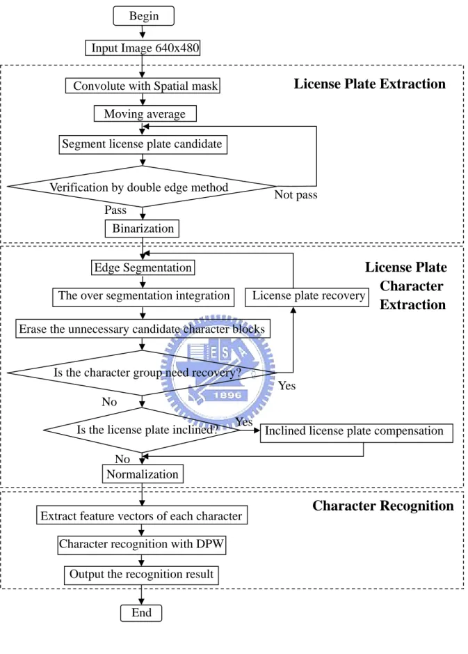
Fig 1.1 The flowchart of the LPR system in this thesis.………5

Fig 2.1 The gray level distribution of a character vertical stroke………..8

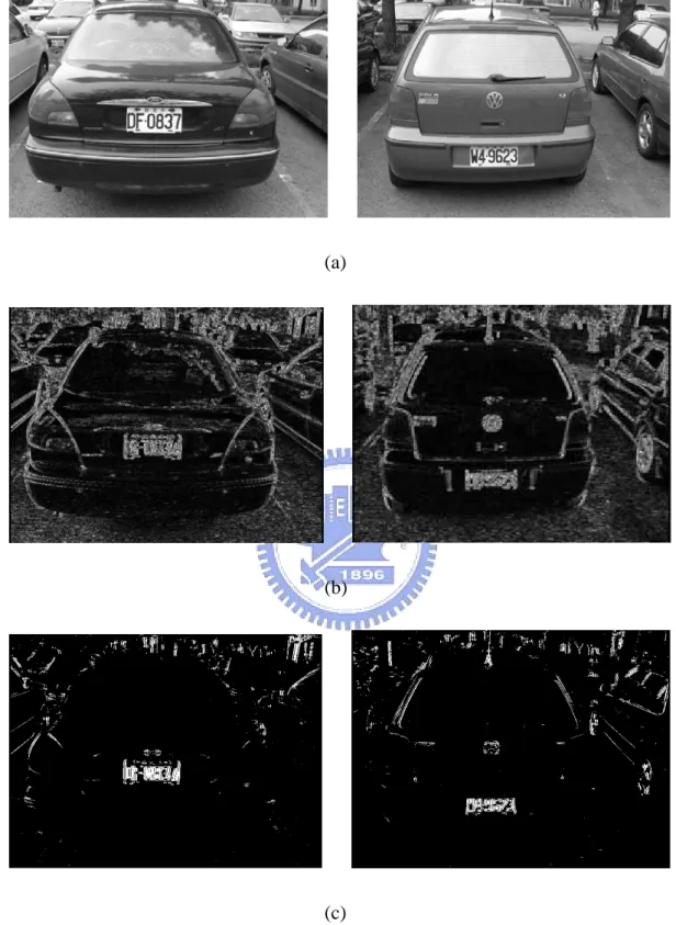
Fig 2.2 (a) original images, (b) Spatial domain images and (c) binary image………...9

Fig 2.3 (a) Binary of spatial domain images, (b) results of moving average, and (c) binary images……….12

Fig 2.4 Rough license plate segmentation by projection……….14

Fig 2.5 License plate candidates………..14

Fig 2.6 Incorrect license plate candidates………15

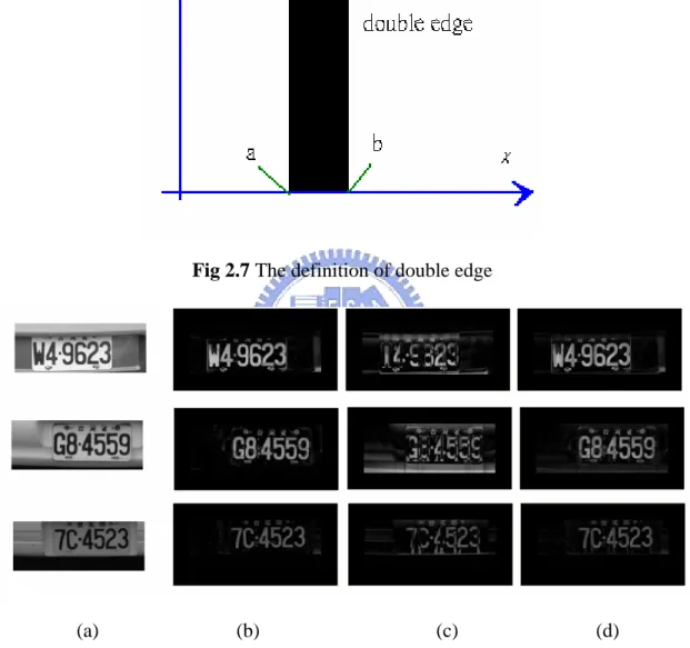
Fig 2.7 The definition of double edge………..17

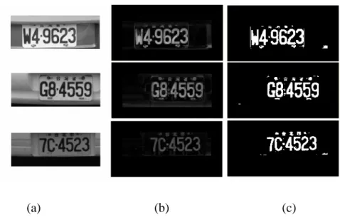
Fig 2.8 The double edge result, (a) the original images, (b) the result of the horizontal double edge, (c) the result of the vertical double edge, and (d) the finally result………...17

Fig 2.9 The double edge result (a) the original result, (b) the result of double edge, and (c) the binary image of double edge……….18

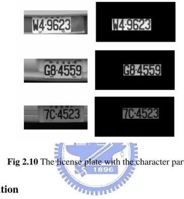
Fig 2.10 The license plate with the character part………...19

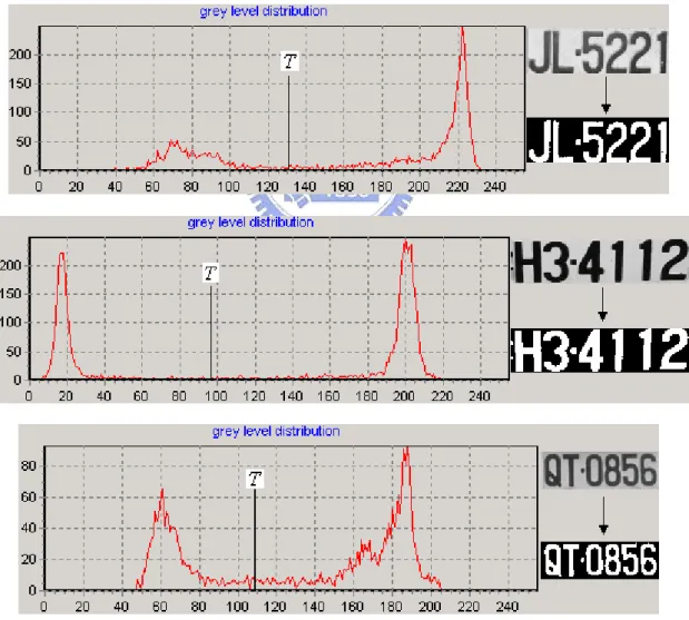
Fig 2.11. the grey level distribution of character groups and the related binary images ………...……….20

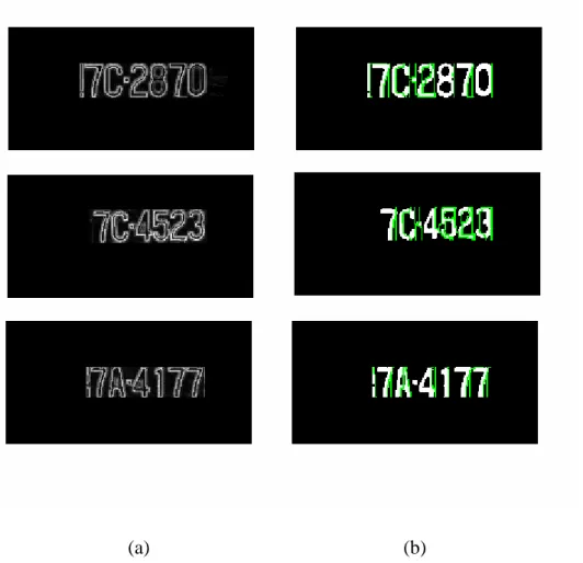
Fig 3.1 (a) the original license plate, and (b) the result of the character edge detection

………24

Fig 3.2 (a) the spatial domain image of edge, and (b) the segmentation result, and the green lines are the segmentation path………28

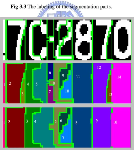
Fig 3.3 The labeling of the segmentation parts………30

Fig 3.4 Integrating with the parts that with little white points………….………30

Fig 3.5 The Integrating result………...32

Fig 3.6 The erasing result……….34

Fig 3.7 Erase the repeat candidate character blocks………35

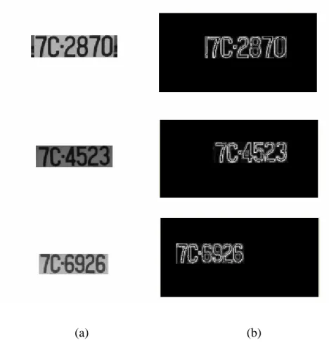
Fig 3.8 Compare edge segmentation method with projection method and connected component segmentation. (a) The edge segmentation method, (b) the projection method, and (c) the connected component segmentation ………36

Fig 3.9 License plate recovery……….37

Fig 3.10 Inclined license plate compensation………..38

Fig 4.1 The minimum cost related to the optimal path………42

Fig 4.2. Aircraft routing network and the minimum-fuel cost from city a to each other ………45

Fig 4.3 The RAV curve of each reference character………47

Fig 4.5. The “path” of (4.13) ………51

Fig 4.6. A comparison between the reference character and the shifted character image and their related CAV1s……….….52

Fig 4.7 The “path” of a shifted input ϕ_xc1………...53

Fig 4.8 Three allowed sub-path in DPW………..54

Fig 4.9. The legal region of the path………56

Fig 5.1 The input grey-level images and the extracted license plates ……….60

Fig 5.2 The three images failed in license plate extraction step………..61

Fig 5.3 The successful examples of the license plate character extraction ………….62

Tables

Table 3.1 Normalized character templates……….……..39 Table 4.1 The value of important parameters……….……..57 Table 5.1 The different contrast and blur of license plate images………64 Table 5.2 The license plate character extraction rate in the four conditions…………64 Table 5.3 The accuracy of each kind of extraction methods………65 Table 5.4 The number of each alphanumeric character extracted from input images ………..66 Table 5.5 The number of each numeric character extracted from input images……..67

Chapter 1

Introduction

1.1 Preliminary

Recently, more and more investigators have paid attentions to the Intelligent Transport System (ITS), in which the license plate recognition (LPR) plays an important role and has been widely used in numbers of applications, such as unattended parking lots, security control of restricted areas, traffic law enforcement, and automatic toll collection. Therefore, the license plate recognition has become a significant topic in research.

In general, the LPR system can be separated into three steps. First step is extracting the license plate, which could be implemented by methods based on morphology [5][18] and neural networks [14]. Second step is extracting the characters from the license plate, processed by several methods, for examples the projection method [16][7]. However, the character extraction rate will be influenced by the low contrast or blur of the license plate images. Hence, in this thesis, a method called Edge Segmentation method is proposed to enhance the accuracy of the license plate character extraction. The final step is recognizing the characters, which most of the investigators have worked on, and derived a lot of algorithms, such as the template

matching method [3] and neural network [4]. It is known that the recognition rate could be directly influenced by the detecting and recognizing processes. Besides, some physical factors will impair the recognition rate, such as varying illumination outdoors, blurring image of a moving vehicle, dirty or inclined license plates, and so forth. In order to achieve a higher recognition rate, it is required to deal with the above problems. The following section will introduce the problems to be solved in this research.

1.2 Problem Statements

While the LPR system operates outdoors, it is seriously affected by two kinds of problems; one is related to the headlamp or radiator of the vehicles and the other is caused by the illumination variation and the complex texture of vehicles. It has been known that these two problems will highly reduce the recognition rate. In order to effectively design LPR systems, it is necessary to analyze the disturbances in the above problems, which are described as below:

1) Disturbances caused by the headlamp or radiator of vehicles

To achieve a better LPR rate, the license plate must be accurately extracted in the first step of the license plate recognition. Some methods with spatial masks have

been proposed to extract the license plate, but they often encounter a serious problem caused by the vehicle’s headlamp or radiator, whose features abstracted from spatial masks are similar to the license plate. As a result, their algorithms may fail to extract the real license plate. Hence, how to improve the algorithms to alleviate the influence of the headlamp and radiator becomes an important problem.

2) The disturbances caused by the illumination variation and complex texture of vehicles

In an outdoor environment like roadways or highways, the varying illumination and the complex texture of vehicles could easily cause the mistakes in the second step of the LPR system, license plate characters extraction. The same problem also exists when the license plate is dirtied. These interferences will make the characters extraction over-segmented or under-segmented, and finally, will reduce the accuracy of the LPR system. Therefore, how to enhance the extraction rate will be an important problem in this thesis.

In order to improve the above drawbacks, this paper employs the double edge method to reject the disturbances caused by the vehicle headlamp or radiator, which will be introduced in next chapter. Besides, the edge segmentation method is proposed to deal with illumination variation and complex texture of vehicles, and it will be

mentioned in Chapter 3. In addition, an efficient character recognition approach incorporated with Dynamic Projection Warping methods will be introduced in Chapter 4.

1.3 The Three Steps of the LPR System

In this section, the methods used in the three steps of the LPR system, license plate extraction, license plate character extraction and character recognition, in this thesis are shown in Figure 1.1. In the first step of the license plate extraction, the spatial mask and moving average are utilized to strengthen the feature of the license plate, and the double edge method is proposed to the verification of the license plate candidates. In the license plate character extraction process, the edge segmentation method is developed to extract the license plate character well. Finally the DPW method is applied to the character recognition. The detail introduction of the license plate extraction, license plate character extraction and character recognition are mentioned in Chapter 2, Chapter 3 and Chapter 4 respectively.

Begin

Input Image 640x480 Convolute with Spatial mask

Moving average

Segment license plate candidate Verification by double edge method

Not pass Pass

Binarization Edge Segmentation

The over segmentation integration Erase the unnecessary candidate character blocks

Is the character group need recovery?

Yes

License plate recovery

No

Is the license plate inclined? Yes Inclined license plate compensation Normalization

Extract feature vectors of each character Character recognition with DPW

Output the recognition result No

Character Recognition

License Plate

Character

Extraction

License Plate Extraction

End

Chapter 2

The License Plate Extraction

2.1 Introduction

Generally, the procedure of the LPR system usually consists of three steps, license plate extraction, character extraction and character recognition. The first step of the LPR system is the license plate extraction. In the past two decades, several techniques of license plate extraction had been proposed such as color extraction method [9], symmetry [8], vertical edges [11], spatial mask [20] [22], and so on. In this thesis, the used methods of the license plate extraction are spatial mask [22], moving average, candidate segmentation, double edge method, and the binarization. Usually, the lamps and the radiators of vehicles reduce the extraction rate because of the similar features to the license plates with the spatial mask. Fortunately, a method, double edge, is found to solve the problem cause by the lamps and the radiators, and the double edge method will be introduced in section 2.5. Then the following sections will present the process of the license plate extraction and chapter 3 and chapter 4 will introduce the character extraction and character recognition.

2.2 Spatial Mask

It is known that the spatial mask is a fundamental technology to abstract features in gray-level or color images, such as vertical objects and horizontal objects [22]. Hence, a color image to be processed with spatial mask should be changed to gray-level first. In this thesis, the spatial mask will be adopted to find the feature of vertical strokes, which are needed for extracting the license plate. Since the images processed here are color images, they should be changed to gray-level before the spatial mask is used.

The first step of the LPR system is to extract the license plate, which is regarded as a white rectangular metal plate and contains black characters set including two alphanumeric characters and four numeric characters. In this paper the spatial mask is utilized to filter out character vertical strokes. Usually, the character stroke is 5 pixels in width for a license plate about 110x40 pixels, and figure 2.1 illustrates the distribution of a character vertical stroke in gray level image. Then a spatial mask h is shown as below

[

−1 −1 −1 1 4 1 −1 −1 −1

]

= , , , , , , , ,

h (2.1)

which is designed to enhance the black vertical strokes from the white background. Let f be the input gray level image and g is the output image in spatial domain; the relation between image f and image g can be expressed as followed

( )

, |

( ) (

,

)

| 4 4

∑

− = + = k y k x f k h y x g (2.2)

where h(k) is the k-th element of h, −4≤k≤4, and and represent the gray level of the pixel at (x,y) in the input image and the spatial domain image, respectively. However, after the spatial mask the result, g, may not be a value between 0 and 255, a range for gray-level. In order to process g conveniently, g should be linearly normalized to be gray-level and shown in an image as Fig 2.2(b). Then, for selecting correct vertical strokes, a threshold T is set to binarize the resulted image of

g and an output binary image is obtained as

) , (x y f g(x,y) (2.3)

( )

( )

⎩ ⎨ ⎧ > = otherwise 0 255 g x,y T y x, b

where 255 represents the point of a vertical stroke, and 0 represents a useless point. Figure 2.2 shows the result of the spatial mask and binary image. In this thesis, the threshold T of (2.3) is set as 128, the middle value. In the Figure 2.2(c), there are still some white portions existing that don’t belong to the license plate and cause by the shadow and background. The following section will explain the method, moving average, which is used to remove useless white portions.

(a) (b) (c)

2.3 Moving Average

Generally, the moving average is used to filter out the noise in the image, but it blurs the image. Although the image would be blurred, but moving average is utility for eliminating the noise from the mage. Hence, in this thesis, we still use moving average to filter out the noise.

Consider the binary image Fig.2.2(c), which is the result after the spatial mask and contains many useless white portions caused by the background or the shadow. However, these useless portions are usually treated as noise, which are broken, small and of low density when compares to the portions belonging to the license plate. Hence, the moving average can be used to suppress the unnecessary portions, and the moving average function is shown below

2 ) , ( ) , ( k j y i x b y x M k k i k k j

∑ ∑

− = =− + + = (2.4)

where M is the result image of the moving average and k is the width of the window. In this thesis, k is set as 5, and Figure 2.3(b) shows the result of the moving average. Finally, the same with the spatial mask, for selecting correct portions, a threshold Tm is set to binarize the resulted image of M and an output binary image is obtained as

(2.4)

( )

( )

⎩ ⎨ ⎧ > = otherwise 0 y x, 255 y x, m m T M b

where 255 represents the point of a vertical stroke that locate in the license plate, and 0 represents a vertical stroke cause by the shadow and background and useless point.

Figure 2.3(c) shows the result binary image, bm. In this thesis, the threshold Tm of (2.4) is set as 102, an experiential value. After the spatial mask step and moving average step, the characteristics of the license plate have been choose, then the next section will show how to use these characteristics to select the license plate from the whole image.

(a) (b) (c)

Fig 2.3 (a) Binary of spatial domain images, (b) results of moving average, and (c) binary images.

2.4 License Plate Candidate Segmentation

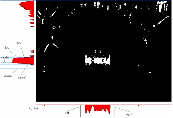
Generally speaking, the license plates are located at the lower part of a car. Hence searching the license plate in the direction from down to top is easier and more efficient. Besides, the lower part of image has few noises such as lamps, symbols, radiators, etc. Base on these concepts, a method called projection extraction method is used to rough license plate segmentation. In this thesis, the license plates are from 90x30 pixels to 130x50 pixels, so in this step choose a rough range 160x60 that can complete include a license plate. First, use the y-axis projection to search the and , and Figure 2.4 shows the location of and . Because of the slant of the license plate, the range from to may cut the license plate. Hence choose the location with largest projection value between and be the center of the license plate, , and choose and with the following equation ' top P ' down P Ptop' Pdown' ' top P P_down' ' top P P_down' center P Ptop Pdown 30 − = center top P P 29 + = _center down P P (2.5)

which the range from Ptop to Pdown is 60 pixels.

Then by utilizing the x-axis projection of the selected vertical range of image, the detected license plate left and detected license plate right will be selected as below,

left

(2.6) ( ) X Proj

[

i j P j i left =

∑

+ = ∈ 159 0 640 , 1 _ max

]

160 + = left right P P (2.7)

where is the accumulated value of i-th column of the selected vertical range of image. Figure 2.5 shows the result of the projection method, but sometimes the method will cause a wrong result because of the lamps, radiators, etc. Figure 2.6 shows the wrong result cause by the lamps and the radiators. Therefore, the next section will introduce how to use the double edge method to determine if the range including a license plate, and to extract the license plate accurately.

[ ]

i Proj X _

Fig 2.4 Rough license plate segmentation by projection

Fig 2.6 Incorrect license plate candidates

2.5 Double Edge Method

The strokes of the license plate characters are about 5 pixels in this thesis, so an algorithm using in the background removal is chosen to find the less than 5 pixels strokes in the license plate candidates. This thesis proposes a method, called double edge method, to extract the license plate characters, which is similar to the method introduced by Xiangyun Ye, Mohamed Cherret, and Ching Y. Suen [19]. Based on the double edge method, whether a candidate is a license plate or not can be determined. The double edge method regards a pixel with the following characteristics as an object pixel

1) it has a gray level lower than that of its local neighbors;

2) it belongs to a thin connected component with width less than a predefine value.

Then the definition of the double edge is shown as follows

(2.8) ⎩ ⎨ ⎧ < < = elsewhere 0 if 1 ) ( , b x a , y x, f

where 1 represents the point that belong to the edge, and 0 represent the point that belong to the background. Then a and b are the boundaries of the edge as shown in

Figure 2.7. In a one-dimensional profile, a stroke with thickness less than W can be treated as a double edge stroke, whose intensity is

) ( ))} ( ), ( ( { ) (x Max Min f x i f x W i f x I W 1 1 i DE = =− − + − − (2.9)

where f is the gray scale value of the point. In this thesis, the two-dimensional double edge strokes are more useful in character segmentation and recognition. Therefore use the one-dimensional double edge method in horizontal and vertical to set up the two-dimensional double edge strokes. The relation between horizontal double edge and vertical double edge is as following

(2.10) ) ( ) ( ) ( ) (x,y γI x,y 1 γ I x,y IDE = DEd=0 + − DEd=1

where d=0, 1 refer the two directions, and γ is the ratio between horizontal double edge strokes and vertical double edge strokes. In this thesis the horizontal double edge is more important than the vertical, so γ is set as 0.75. Figure 2.8 shows the result of the double edge, and in this thesis the W is set as 15. Then, the binarization still has to do in this part in order to select the strokes of the characters, and the function is shown below (2.11) ⎩ ⎨ ⎧ > = ortherwise 0 ) ( if 255 ) ( , y x, I , y x, b DE DE T

where 255 and 0 respectively represent the pixel (x,y) is in a stroke and within the background. Besides, )} ( {I x,y Max T =λ _DE (2.12)

where λ represents the ratio to choose the threshold, and λ is set as 0.333 in this thesis. Then Figure 2.9 shows the result of the double edge, and continues white points are shown as a stroke of the characters.

Fig 2.7 The definition of double edge

(a) (b) (c) (d)

Fig 2.8 The double edge result, (a) the original images, (b) the result of the horizontal double edge, (c) the result of the vertical double edge, and (d) the finally result.

(a) (b) (c)

Fig 2.9 The double edge result (a) the original result, (b) the result of double edge, and (c) the binary image of double edge

In a license plate, there are six characters and one dash, so in a row of the license plate there are at least 6 strokes and at most 13 strokes. However there exist noise and destruction of the license plate, the range can be change to 4 strokes to 18 strokes in this thesis. Hence a row is seen as a part of the license plate if the number of strokes in the row is between 4 and 18. Similarly, a candidate image is decided to include a license plate if the rows that belong to a license plate are continuous and the number of the row is between 18 and 45. If the candidate doesn’t include a license, then we should return to the license plate candidate segmentation to find another candidate until a candidate is decided to include a license plate. By the result image of double edge method the height of the license plate can be found, and use the x-projection on the binary image of the double edge result to find the width of the license plate.

Figure 2.10 shows the license plate that after the statistics, and we can see that only the character part can be kept. In the next section, the binarization is done to the character part to make the character segmentation and character recognition more easily.

Fig 2.10 The license plate with the character part.

2.6 Binarilization

After extracting the character group from the rough license plate, the binarilization process is usually employed as the pre-process of character recognition. Nevertheless, for different lighting conditions to have a best result the threshold should be different. Many methods of choosing the threshold from a grey level image such as binarilization by average, Ostu’s method [13], etc. According to the grey level distribution of extracted character group image, three examples are given in, the threshold used in this paper is a dynamic value, which is selected by the following steps. Suppose the extracted character group image, denoted as f ,

(

x y

)

, with m×n

pixels, each pixel can be classified to either higher grey level class H or lower grey level class L, and the number of pixels in H is equal to L. Let σ_H and σ_L be the average grey level of H and L respectively, the threshold T is selected as (2.13) and the binary character group image B can be obtained from (2.13).

(

H L

)

T = σ +σ 2 1 (2.13)

( )

( )

_{( )}

⎩ ⎨ ⎧ ≥ < = T y x, f , T y x, f , y x, if 0 if 255 B (2.14)

Three examples of binary images are shown in Figure 2.11.

Fig 2.11. the grey level distribution of character groups and the related binary images.

By the mentioned steps, spatial mask, moving average, double edge method and binarization, the license plate extraction is completely finished. And these steps are also the pre-processing works of the character segmentation and recognition. Hence the following two chapters will introduce the license plate character segmentation and character recognition.

Chapter 3

The License Plate Character Extraction

3.1 Introduction

Although the LPR system is discussed for many years, but the character extraction is seldom mentioned. Usually, the projection [16] and the connected component segmentation [12][17] are used to extract the license plate characters. Unfortunately, some undesired factors will reduce the extraction rate, such as the noise, the illusion, and the destruction or the slant of the license plate. In order to avoid theses undesired factors, this paper presents a novel method called edge segmentation to extract the characters. This method refers to the work by Nafiz, Fatos, and Yarman for the cursive handwriting recognition [1], and modifies their algorithms to extract the character in this thesis. The projection method and the connected component segmentation are used in the binary image, and these two methods rate are influenced by the quality of the binarization very much. In the edge segmentation methods, it is worked on the characteristic image of the edge, so it is seldom influenced by the binarization. Before introducing the edge segmentation in Section 3.3, it is required to detect the character edge, a kind of pre-process similar to the spatial mask, which will be given in Section 3.2.

3.2 Character Edge Detection

Different to the one-dimensional spatial mask method in Section 2.2 for the detection of character strokes, the spatial mask method introduced here is a kind of two-dimensional method and applies to the detection of character edges. The spatial masks chosen for edges in the angles of 0, π/4, π/2, and 3π/4 to be detected are all given as (3.1) ⎪ ⎩ ⎪ ⎨ ⎧ = − = − = − = 1 1 0 2 1 1 ) ( k , k , k , k h_e

which has been commonly used to enhance the edges. Let f be the license plate image in gray level. With the above spatial mask, four images in spatial domain in the angles of 0, π/4, π/2, and 3π/4 can be attained as

| k y x, f k h | y x, g₀

∑

_e − = + = 1 1 ) ( ) ( ) ( k (3.2) | k y k, x f k h | y x, g _/

∑

_e − = − + = 1 1 4( ) ( ) ( ) k π (3.3) | y k, x f k h | y x, g _/

∑

_e − = + = 1 1 2( ) ( ) ( ) k π (3.4) | k y k, x f k h | y x, g _/

∑

_e − = + + = 1 1 4 3 ( ) ( ) ( ) k π (3.5)

where f(x,y) represents the gray level value of the pixel at (x,y) and

( )

x,y ∈R=

{

( )

x,y x=0,1,...,159,and y=0,1,...,59

}

. To include all the edge information related to the angles of 0, π/4, π/2, and 3π/4, a new spatial domain image is defined as

( )

x,y

(

g

( )

x,y g ₄

( )

x,y g ₂

( )

x,y g_{3 4}

( )

x,y

)

/4

g_e = ₀′ + _π′_/ + _π′_/ + ′_π/ (3.6)

where g′_a( yx, ) is the normalized from g_a( yx, ), a=0, π/4, π/2, and 3π/4, by

( )

( )

{

( )

}

255 ) ( = ⋅ ′ ∈ g x,y max y x, g y x, g a y x, a a R

Applying (3.6) to the edge segmentation yields the result shown in Figure 3.1. In the next section, the edge segmentation, will introduce how to use the spatial domain image g_e to extract the license characters.

(a) (b)

Fig 3.1 (a) the original license plate, and (b) the result of the character edge detection.

Usually, the character extraction methods in a LPR system are projection method or connected component segmentation. Unfortunately, these methods can only work well if the original images of the license plate are with no slant and with low noise and high contrast. Hence, in this thesis a method called edge segmentation is presented to extract the license characters avoiding the influences mentioned above. This method refers to the work by Nafiz, Fatos, and Yarman for the cursive handwriting recognition [1], and modifies their algorithms to extract the character. The edge segmentation method in this thesis can be separated into the following two steps:

1) Setting the start points to find the segmentation paths

In this thesis, the characteristic values corresponding to the right edge and the left edge of a stroke are used as important data to segment the characters of a license plate, and to avoid cutting the next character, respectively. In this step the binary image of a license plate is required to set the start points of the segmentation paths, which will be determined in the next step. There are two groups of the start points, respectively located at the horizontal lines in the 1/3 and 2/3 height of the binary image. The reason to choose these two groups is that the curvy strokes of 2, 5, 6, 9, C, G, and S complicate the segmentation paths, which will be explained in the next step. If a point at the horizontal lines is of gray value 255 and next to a point on the right of gray

value 0, then this point is set as a start point. Label the locations of all the start points at the spatial domain image correspondingly. Next, the segmentation paths will be found on the spatial domain image based on the locations labeled as the start points.

e

g

e

g

2) Determining the segmentation paths

In this step, the spatial domain image is used to find the segmentation path. The segmentation path can be separated into two parts: one is over each of start lines; the other is under the start lines.

e

g

a) The segmentation path over the start line

In over start line part, the segmentation path growing directions from the start points are 0, π/4, and π/2, and the reason to choose the three direction is to avoid the segmentation path growing to the under direction. The segmentation path growing direction is chosen the following equation

(

)

(

)

(

)

(

) (

)

(

)

(

)

(

)

(

)

(

) (

)

(

(

)

(

)

⎪ ⎪ ⎪ ⎪ ⎪ ⎪ ⎩ ⎪⎪ ⎪ ⎪ ⎪ ⎪ ⎨ ⎧ − > − + − > − + + > − + − + > + − > + − + > + + = ′ ′ otherwise and if and if , 1 y x, T 1 y 1, x g , 1 y x, g 1 y 1, x g , y 1, x g 1 y 1, x g , 1 y 1, x T y 1, x g , 1 y x, g y 1, x g , 1 y 1, x g y 1, x g , y 1, x y , x _{e e} e e e e e e e e e e

)

(3.7)

large enough to be considered as a part of edge, and in this thesis Te is set as 50. Originally, the point (x,y) in (3.7) is one of the location of the start points, and with (3.7) the next point of the segmentation path can be find as (x ′′ ). Then let (,y ) be (x,y) to do (3.7) again until the locations of

y , x ′′ x′ or y′ is the left boundary or the top

of the license plate.

b) The segmentation path under the start line

The method to find the segmentation in this part is almost the same with the over part, but the growing direction is 0, 7π/4, and 3π/2. The way to grow the segmentation path in the under part is

(

)

(

)

(

)

(

) (

)

(

)

(

)

(

)

(

)

(

) (

)

(

(

)

(

)

⎪ ⎪ ⎪ ⎪ ⎪ ⎪ ⎩ ⎪⎪ ⎪ ⎪ ⎪ ⎪ ⎨ ⎧ + > + + + > + + + > + + + + > + + > + + + > + + = ′ ′ otherwise and if and if , 1 y x, T 1 y 1, x g , 1 y x, g 1 y 1, x g , y 1, x g 1 y 1, x g , 1 y 1, x T y 1, x g , 1 y x, g y 1, x g , 1 y 1, x g y 1, x g , y 1, x y , x _{e e} e e e e e e e e e e

)

(3.8)

The same with (3.7), originally, the point (x,y) in (3.8) is one of the location of the start points, and with (3.8) the next point of the segmentation path can be find as ( ). Then let ( ) be (x,y) to do (3.8) again until the locations of or is the left boundary or the foot of the license plate.

y ,

x ′′ x ′′,y x′ y′

Observing (3.7) and (3.8), it is shown that if there is only one group of the start points, then the segmentation paths will cut the curvy strokes when the path growing

to the curvy strokes of characters 2, 5, 6, 9, C, G, and S because of the growing directions of each part. However, the right boundary of characters with curvy strokes is on the 1/3 or 2/3 height of the characters. Hence there must have two groups of the start points to avoid cutting the curvy strokes, and Figure 3.2 shows the segmentation result.

(a) (b)

Fig 3.2 (a) the spatial domain image of edge, and (b) the segmentation result, and the green lines are the segmentation path.

In Fig 3.2, it shows that there may be more than one segmentation path in a character, because there may be more than one start points in a character. Hence, with the edge

segmentation method, the segmentation is usually ‘over segmentation’, and next section and Chapter 4 will introduce how to integrate the over segmentation parts and how to use the DPW recognition method to get the license plate recognition result.

3.4 The Over Segmentation Integration

In this section, the segmentation paths should be labeled on the binary image of the license plate first. After the process of edge segmentation method, a character may be separated into 4 parts at most. Hence, in this section the over segmentation part will be integrate to find the complete character, and the integration process can be also separated into two steps:

a) Labeling the segmentation part in order

In the edge segmentation result, the license plate is separated into many parts, and a character may be separate into 4 parts at most. So, we just have to combine four parts at most to find a complete character, and the labeling method is shown as Fig 3.3. In Fig 3.3 we take one of the license plates for example. The labeling order of the segmentation part is up to down and left to right, and it can be observe clearly in Fig 3.3. However, some segmentation part only with little white points which are the character strokes. Therefore, in order to decrease the segmentation parts, these parts are integrated into the last order parts. The integrating result is shown in Fig 3.4.

Obviously, compare Fig 3.3 and Fig 3.4, the number of segmentation parts is decreased, and this will help reduce time in the recognition process.

Fig 3.3 The labeling of the segmentation parts.

b) Integrating the segmentation parts

With the edge segmentation method, a character block may be separated up to 4 sub blocks. Hence the integrating process should combine 1, 2, 3 or 4 segmentation parts, and work in the labeling order. The first character block, put label 1 to be a candidate character block, second put label 1 and 2 together to be a candidate character block, third combine label 1, 2 and 3, forth combine label 1, 2, 3 and 4, and then put label 2 to be a candidate character block and so on. Hence, if there are n segmentation parts, there will be 4(n-3)+6 candidate character blocks. However, the width of the license plate character is limited, so a candidate character with width bigger than is not to be considered as a character. In this thesis, is set as 45, and Fig 3.5 shows the integrating result. After the integrating process, there are still many candidate character blocks, and the next section will introduce how to reduce the candidate character blocks and to retain the candidate character blocks that contain a complete license plate character.

w

Fig 3.5 The Integrating result.

3.5 The Candidate Character Blocks Erasing by the Character

Factors

Some of the candidate character blocks are not a complete character or include more than one character because of the over-segmentation by the edge segmentation method. In order to erase these candidate character blocks, some character factors coefficient will be set as the following two points.

a) The ratio of the character height and width.

The ratio of the character height and width is limited because the measure of the license plate characters is ordered. The license plate characters can be separated into

two types, one type just includes character ‘1’ and ‘I’, the other type includes the other characters. In the first type, the ratio of height and width is between 3.5 and 4, and in the other type, the ratio of height and width is between 1.8 and 2.3. Then a candidate character block will be not seen as a character if the ratio of its height and width is not between 3.5 and 4 or 1.8 and 2.3.

b) The density of the character.

The same with the a) part, the density of the license plate characters can be separate into these two types. The density of the first type is between 0.55 and 0.63, and the density of the other type is 0.4 to 0.62. Hence, a candidate character block will be not seen as a character if the density is not between 0.55 and 0.63 or 0.4 and 0.62.

Before using the above coefficients to erase the candidate character blocks, the region growing is used in each candidate blocks to divide each uncorelation part. Then use the a) and b) features of character to decide if the uncorelation part is considered as a character or not, and Fig 3.6 shows the erasing result.

Fig 3.6 The erasing result.

After the integrating process and erasing process, only the uncorelation parts that conform to the character factors are kept, and the number of candidate character blocks is reduced. However, consider Fig 3.6, there still exist many candidate character blocks that include the same character because of the over-segmentation of the license plate characters. Then the next step is to erase the repeat uncorelation parts and the repeat candidate character blocks. Let A be one of the candidate character blocks, and B be another candidate character block. If A is

included in B, then A can be erased, and Fig 3.7 shows the result. Finally, the license plate character extraction is done, and Fig 3.8 will shows a license plate that the characters can be extract by the edge segmentation but can’t be extract by the projection method or connected component segmentation.

(a) (b) (c)

Fig 3.8 Compare edge segmentation method with projection method and connected component segmentation. (a) The edge segmentation method, (b) the projection

method, and (c) the connected component segmentation.

In Fig 3.8, the license plate is with low contrast and with a slant angle. Hence, the binary of the license plate characters many be linked, such like the characters ‘6’ and ‘0’ in Fig 3.8. Hence, the projection method and connected component segmentation will get the wrong result, and usually under-segmentation.

3.6 License Plate Recovery and Inclined License Plate Compensation

When characters are extracted out, some additional and necessary information of license plate and characters are also obtained. Given Figure 3.9 as an example of license plate recovery [21], if any boundary of character is on the boundary of the extracted character group image, it means that perhaps some pixels of the character are outside the character group image. Consequently, that boundary of character group image will be extended one pixel and characters will be extracted by edge segmentation method again. Repeat the above until every character is well-extracted.

Fig 3.9 License plate recovery

Due to the angle of camera capturing images, the extracted license plate is sometimes inclined with a small angle less than 10°. In order to have a better character recognition rate, an inclined license plate compensation procedure [18] is required. Let be the inclined license plate with its width and let

(

)

be the center of . In addition, let be the height difference between the centers of the first and the last characters of . Then, the compensated license plate image can be obtained from the following equation. Figure 3.10 shows the example of inclined license plate compensation.

p R w_R x ,_c y_c p R D_R p R p R′

( )

p

(

(

c

)

R R

)

p x y R x y x x D w R′ , = , − − * / (3.9)

Fig 3.10 Inclined license plate compensation

3.7 License Plate Character Normalization

Since the characters extracted out from different license plates are generally in different sizes which will make the character recognition more difficult, it is necessary to normalize the characters to a fixed size. By using the normalization method, all the characters processed in this paper is normalized to 30×15 pixels, such as the character templates in Table 3.1 However, the images received by CCDs often contain undesired noise caused by varying illumination, blurred effect, dirty plate, and fragmented characters. As a consequence, it is rather difficult to perfectly extract the characters out, and most importantly, the recognition rate may be reduced to a certain level. To tackle the above problem, this paper utilize a method, called dynamic projection warping (DPW), which will be introduced in the next chapter.

Table 3.1 Normalized character templates

Character Template Character Template Character Template

0 C P 1 D Q 2 E R 3 F S 4 G T 5 H U 6 I V 7 J W 8 K X 9 L Y A M Z B N

Chapter 4

License Plate Character Recognition

After the license plate extraction and license plate character extraction, the final step of the LPR system is the character recognition. In this thesis, the character recognition method refers to the recognition method, DPW [18]. In Section 4.1, first I will introduce the DPW method, in Section 4.2 the feature vector of character recognition is mentioned, and finally in Section 4.3, how to use DPW in the character recognition will be explained.

4.1 Introduction

Generally speaking, basic recognition method of recognizing the license plate characters could reach the recognition rate, 80% per character, for example 85% per character for the template matching method. However, the above recognition rate is only for clearly characters, which means with no noise and no destruction. In practice, a clearly character is hard to get in outdoor environments like roadways or highways, and the license plate character may sometimes be soiled, dirty or blurred. These characters usually have fragmented strokes, undesired shifted image, pared character images, or unwell-normalized images, etc. The recognition rate of these characters

may be reduced to less than 70% per character for basic recognition method. The proposed method, Dynamic Projection Warping, which reaches the recognition rate 99% of character recognition, would be used in this system, and next section will introduce the feature vector of the DPW.

4.2 Dynamic Programming Technique

Before introduce the DPW in character recognition method, this section will introduce the dynamic programming technique first. Dynamic programming technique has been extensively used in many fields such as speech recognition [10], optimal control [15], etc.

To illustrate the applicability of character recognition, a typical problem, called the optimal path problem, will be stated and discussed here. An example to explain the fundamental concept of the optimal path problem is given in Figure 4.1, which consists of N points labeled orderly from 1 to N. Besides, the cost moving directly from the i-th point to the j-th point in one step is represented by a nonnegative function ς

(

i,j

)

. The path from point 1 to point i may have many selections and leads to different costs. As a result, there should exist a minimum cost, denoted as ϕ

( )

1,i .

Fig 4.1 The minimum cost related to the optimal path

Using traditional terminology, the decision rule for determining the next point to be visited after point i is called a “policy”. Since the policy determines the sequence of points traversed from the (fixed) originating point 1 to the destination point i, the cost is therefore completely defined by the policy and the destination point

i. The question is what policy leads to the function ϕ

( )

1i, .

This principle of optimality, which is the basis of a class of computational algorithms for the above optimization problem, is according to Bellman [2],

An optimal policy has the property that, whatever the initial state and decision are, the remaining decisions must constitute an optimal policy with regard to the state resulting from the first decision.

computation algorithms, consider first moving from the initial point 1 to an intermediate point j in one or more steps. The minimum cost, as defined, is ϕ

( )

1,j . Since moving from point j to point i in one step incurs a cost ς

( )

j i, , the optimal policy, which determines which intermediate point j to pass through, (should one exist) satisfies the following equation

( )

1i

[

( ) ( )

1 j j i

j , ,

min

, ϕ ϕ

]

ϕ = + (4.1)

Generalizing (4.1) to the case in how to obtain the optimal sequence of moves and the associated minimum cost from any point i to any other point j, the following equation can be derived from (4.1)

( )

i j

[

( ) ( )

i l l j

l , ,

min

, ϕ ϕ

]

ϕ = + (4.2)

where ϕ

(

i,j

)

is the minimum cost from i to j in as many steps as necessary. (4.2) implies that any partial, consecutive sequence of moves of the optimal sequence from

i to j must also be optimal, and that any intermediate point must be the optimal point

linking the optimal partial sequences before and after that point.

To actually determine the minimum cost path between points i and j, in any number of steps, the following simple dynamic program would be used:

( ) (

1,l 1,l

)

1 ς ϕ = l =1,2,_K,N

( )

1l

[

( ) ( )

1 k k l

]

k 2 , minς , ς , ϕ = + k =1,2,_K,N N 2 1 l = , ,_K,

M

( )

1l

[

( ) ( )

1 k k l

]

k S , minς , ς , ϕ = + k =1,2,_K,N l =1,2,_K,N

( )

i j _s

(

i j S s 1min , , ϕ

)

ϕ ≤ ≤ = ⇒ (4.3)

where ϕ_s

( )

i,l is the s-step best path from point i to point l, and S is the maximum number of steps allowed in the path.

For a well-known aircraft routing problem illustrates in Figure 4.2, a, b, c, … represent cities, and the numbers represent the fuel required to complete each path. Using the principle of optimality the minimum-fuel problem could be solved easily. First each minimum-fuel cost, ϕ

( )

i,j , can be obtained by (4.3). For example,

( )

a,e =min

[

ς

( ) ( ) ( ) ( ) ( )

a,b +ς b,e,ς a,e,ς a,d +ς d,e

]

=4

ϕ (4.4)

( )

a,e =4

ϕ can be obtained as above. Because any partial, consecutive sequence of moves of the optimal sequence from i to j must also be optimal, the optimal path which is illustrated in red with the minimum-fuel cost from city a to city i, ϕ

( )

a,i =7, can also be obtained.

Fig 4.2. Aircraft routing network and the minimum-fuel cost from city a to each other.

The above is the introduction about dynamic programming technique, and this is the basic structure of the DPW method. Then the following section will set the feature vector of the DPW in this thesis.

4.3 Feature Vector of Character Recognition

The basic concepts of DPW are choosing projection accumulated vector of characters as feature vectors and applying these to dynamic programming method for

recognizing characters.

After the normalization, suitable feature vectors, which represented by a set of character features, have to be adopted for describing the character patterns that will be recognized. Projection accumulated vectors which reduce the dimension from 2-D image to 1-D curve are often adopted to be feature vectors in many LPR researches [6]. In the DPW method, it uses Projection Accumulated Vector, PAV in brief, as the feature vector, which can be decomposed into Column Accumulated Vector, CAV in brief, and Row Accumulated Vector, RAV in brief, defined as

( )

( )

[ ][ ]

(

)

[ ][

]

⎪ ⎪ ⎩ ⎪⎪ ⎨ ⎧ − = − = =

∑

∑

= = 30 1 15 1 j 30 k i k n i j i i i chr CAV chr RAV PAV (4.5)

where chr, m×n pixels, 30×15 pixels for this paper, is the binary image of the extracted character and chr[i][j] is the binary value of pixel (i,j). It is easy to find that CAV is a 15×1 vector and RAV is a 30×1 vector. Consequently, PAV is a 45×1 vector. Figure 4.3 and Figure 4.4 illustrates the RAVs and CAVs of each reference. With the use of PAV, the dimension of the characteristic vector is extended to 30+15=45. Consequently, the higher dimension makes the recognition easier and enough to classify different characters.

Fig 4.3 The RAV curve of each reference character

However, in the Figure 4.3 and 4.4, the PAV of the references may sometimes be similar in CAVs or RAVs, such that ‘L’ and ‘J’ are similar in CAV and ‘M’ , ’N’, and ‘U’ are similar in RAV. In order to discriminate each character more clearly, the definition of PAV could be changed as,

( )

( )

[ ][ ]

(

)

[ ][

]

⎪ ⎪ ⎩ ⎪⎪ ⎨ ⎧ ≤ ≤ − = − ≤ ≤ = =

∑

∑

− = − = 45 31 30 30 1 10 1 0 5 5 i i k chr n i CAV i j i chr i RAV i PAV _l l k l l l l l , , * ) *( 1 * 1) *( j (4.6)

where l=1,2,3 and PAV1, PAV2, and PAV3 satify (4.6),

( )

i PAV₁

( )

i PAV₂

( )

i PAV₃

( )

i

PAV = + + (4.7)

The difference between (4.5) and (4.7) is that in (4.5) the RAV and CAV is according to the whole character and in (4.7) that RAV and CAV is according to the 1/3 width and 1/3 height of the character. Hence the feature vector, PAV, of each character would be more different, and the dimension of the characteristic vector is extended to 30*3+15*3=135. Then how to use DPW in the character recognition will be introduce in the next section.

4.4 Dynamic Projection Warping

In the previous sections, PAV which represented by a set of projection accumulation features and dynamic programming technique have been discussed. This section discusses how to integrated dynamic programming technique with the

feature vector PAV for character recognition. The first subsection states that how to apply dynamic programming technique to the PAV for character recognition. Next, consider the disturbances of real LPR system, some constraints is proposed to constraint the “path” discussed in the previous section. Combining these constraints, the DPW method becomes complete for character recognition.

4.4.1 Fundamental Concepts of DPW

This subsection expresses the integration of dynamic programming and PAV for character recognition. The pattern recognition always utilizes either maximum correlation or minimum dissimilarity classifying patterns.

Before formal introduction of the fundamental concept of DPW, for convenience, the CAV and RAV of a character respectively denoted as ϕ_xcl and ϕ_xrl, shown in (4.8).

( )

( )

( )

[ ][ ]

(

)

(

)

[ ][

]

⎪ ⎪ ⎩ ⎪⎪ ⎨ ⎧ − = − = − = = =

∑

∑

− = − = l l k xl xcl l l xl xrl xl i k chr i CAV i j i chr i RAV i i PAV _* ) *( * ) *( j 10 1 10 5 1 5 30 30 30 ϕ ϕ (4.8)

where l equals to 1, 2, and 3. The CAV and RAV of reference characters are respectively denoted as ϕ and _ycl ϕ , shown in (4.9). _yrl

( )

( )

( )

[ ][ ]

(

)

(

)

[ ][

]

⎪ ⎪ ⎩ ⎪⎪ ⎨ ⎧ − = − = − = = =

∑

∑

− = − = l l k yl ycl l l yl yrl yl i k ref i CAV i j i ref i RAV i i PAV _* ) *( * ) *( j 10 1 10 5 1 5 30 30 30 ϕ ϕ (4.9)

where ref, m×n pixels, 30×15 pixels for this paper, is the binary image of the reference character and ref[i][j] is the binary value of pixel (i,j). Ignoring the shifting, scaling, paring and fragmenting of the extracted character images caused by disturbances, d_l

( )

i,j , dϕcl

(

chr,ref

( )

k

)

, dϕrl

(

chr,ref

( )

k

)

and dϕl

(

chr,ref

( )

k

)

will

be defined as (4.10), (4.11), (4.12) and (4.13)

( )

i,j

( )

i

( )

j i, j dl = PAVxl −PAVyl = (4.10)

( )

(

)

_∑

( )

( )

= − = 30 1 i xrl yrl rl , k i i d_ϕ chr ref ϕ ϕ (4.11)

( )

(

)

_∑

( )

( )

= − = 15 1 i xcl ycl cl , k i i d_ϕ chr ref ϕ ϕ (4.12)

( )

(

)

(

( )

)

(

( )

)

_∑

= = + = 45 1 i l cl rl l , k d , k d , k d i,i

d_ϕ chr ref _ϕ chr ref _ϕ chr ref

( )

)

(4.13) where is the dissimilarity function of 1/3 row or 1/3 column accumulated values between two character images,

(

i,j d_l

( )

(

, k

)

dϕcl chr ref and

represent the total dissimilarity between two RAV

( )

(

chr ref k

)

dϕrl ,

ls and CAVls, respectively, and

is the total dissimilarity between two PAV

( )

(

, k dϕl chr ref

)

)

ls. In the Figure 4.5, take l=1 for example, can be calculated by summing up each

corresponding to the grid point along the “path”, denoted as P.

( )

(

, k

Fig 4.5. The “path” of (4.13)

Unfortunately, the extracted character images usually contain more or less disturbances which cause the images shifted, scaled, pared and fragmented. Hence the “path” has to be changed when the extracted character image contains disturbance. An example to explain how to choose the path is given in Figure 3-6, which illustrated an undesired character image, the under “Z”, which is normalized, over-extracted disturbances in the left two columns and under-extracted right two columns of the upper “Z” in Figure 4.6. It is apparent that ϕ_xc1 which is shown below is almost a curve shifted two columns from ϕ . _yc1

( )

1

(

2

)

1 i = yc i− xc ϕ

ϕ ,3≤ i≤15 (4.14)

Hence, the “path” in Figure 4.5 should be replaced by P’ which is illustrated in Figure

4.7.

Fig 4.6. A comparison between the reference character and the shifted character image and their related CAV1s.

Fig 4.7 The “path” of a shifted input ϕ_xc1

Now, the main disturbances, which resulting from character extraction and normalization such as shifting, paring, and scaling, had been discussed. According to the above examples, each kind of character image has its related path to map the corresponding CAV to the CAV of reference image. Each path can be decomposed

into three kinds of path, P1, P2 and P3, shown in Figure 4.8. Therefore, these three