適用於具指向性天線無線隨意網路之媒介接取控制與路由協定之聯合設計

全文

(1)國立交通大學電信工程學系碩士班碩士論文. 適用於具指向性天線無線隨意網路之媒介接取控制與路由協定之聯合設計. Joint Design of MAC and Routing Protocols for Wireless Ad Hoc Networks Using Directional Antennas. 研究生：謝宜達. Student: Yi-Ta Hsieh. 指導教授：李大嵩博士. Advisor: Dr. Ta-Sung Lee. 中華民國九十三年六月.

(2) 適用於具指向性天線無線隨意網路之媒介接取控制與路由協定之聯合設計. Joint Design of MAC and Routing Protocols for Wireless Ad Hoc Networks Using Directional Antennas 研究生：謝宜達. Student: Yi-Ta Hsieh. 指導教授：李大嵩博士. Advisor: Dr. Ta-Sung Lee. 國立交通大學電信工程學系碩士班碩士論文. A Thesis Submitted to Institute of Communication Engineering College of Electrical Engineering and Computer Science National Chiao Tung University in Partial Fulfillment of the Requirements for the Degree of Master of Science in Communication Engineering June 2004 Hsinchu, Taiwan, Republic of China. 中華民國九十三年六月.

(3) 適用於具指向性天線無線隨意網路之媒介接取控制與路由協定之聯合設計學生：謝宜達. 指導教授：李大嵩博士. 國立交通大學電信工程學系碩士班. 摘要無線隨意網路（wireless ad hoc network）是由多個可任意移動位置之行動主機所組成。為了避免主要由隱藏節點（hidden node）問題所導致的封包衝撞，目前提出的許多媒介接取控制協定採用請求發送/允許發送（RTS/CTS）交換機制以保留媒介給正在傳送或接收的節點。然而當網路負載過重時，許多節點會不必要地被禁止傳輸，而導致網路的整體效能下降。指向性天線由於能將輻射能量集中在某一特定方向，因而顯著地提升了空間再使用的可能性。藉由指向性天線的使用，在鄰近範圍內的二組或以上的節點可同時進行資料傳輸。然而指向性天線的特點卻受到媒介接取控制協定中的媒介保留策略的限制而無法發揮。在本論文中，吾人針對使用指向性天線的媒介接取控制與路由協定提出一整合性的修正。指向性天線具有估測訊號到達方向的能力，因此可利用到達方向的資訊將請求發送/允許發送封包以指向性的方式傳送。如此將僅有在傳輸方向範圍內的節點會被限制傳輸，且這些點並非在所有方向上都受到限制，不僅達成了空間的再使用，也大幅地提升了網路的整體效能。此外，為了能完全發揮指向性天線的特性，吾人提出一能尋找遭受最少干擾路徑之路由策略。利用訊號到達方向可決定與各鄰近節點之相對角度，以及各方向上節點的擁擠程度，如此封包便可經稀疏分佈區域而被送達目的地。最後，相較於使用全向性天線的系統，吾人藉由電腦模擬驗證上述具指向性天線的無線隨意網路系統架構大幅地改進了網路的整體效能。. I.

(4) Joint Design of MAC and Routing Protocols for Wireless Ad Hoc Networks Using Directional Antennas Student: Yi-Ta Hsieh. Advisor: Dr. Ta-Sung Lee. Institute of Communication Engineering National Chiao Tung University. Abstract A wireless ad hoc network is a collection of wireless mobile hosts that are dynamically and arbitrarily located in a certain area. In order to avoid packet collisions which are mainly caused by the hidden node problem, most proposed MAC protocols utilize the RTS/CTS exchanging mechanism to reserve medium for acting nodes. However, in a heavy-load network, lots of nodes are unnecessarily prohibited from transmitting, and the throughput performance goes down accordingly. By focusing energy in an intended direction, directional antennas increase the potential for spatial reuse significantly, and simultaneous data transmissions of two or more pairs of nodes located in each other’s vicinity may be allowed. However, the advantages of directional antennas cannot be exploited under the medium reservation policy in the MAC protocol. In this thesis, we propose an integrated refinement of MAC and routing protocols with the use of directional antennas. Directional antennas have the ability to estimate the direction of arrival (DOA) of an incoming signal. With DOA information available, RTS/CTS packets can be transmitted directionally. Therefore, only those nodes located within the direction of transmission are blocked, and these nodes are not blocked in all directions. Spatial reuse can thus be achieved, and the throughput performance is improved significantly. Furthermore, to fully exploit the advantages of directional antennas, we propose a routing strategy to discover a route that experiences the least interference. The DOA information helps a node to identify the relative directions of its neighbors and the crowd level in all directions. Therefore, packets can be routed to the destination through a sparsely populated area. Finally, we evaluate the performance of the proposed system architecture by computer simulations, and confirm that utilizing directional antennas in ad hoc networks improves the throughput performance greatly over omni-directional communications. II.

(5) Acknowledgement I would like to express my deepest gratitude to my advisor, Dr. Ta-Sung Lee, for his enthusiastic guidance and great patience. I learn a lot from his positive attitude in many areas. Heartfelt thanks are also offered to all members in the Communication Signal Processing (CSP) Lab for their constant encouragement. Finally, I would like to show my sincere thanks to my parents and friends for their invaluable encouragement and love.. III.

(6) Contents Chinese Abstract. I. English Abstract. II. Acknowledgement. III. Contents. IV. List of Figures. VI. List of Tables. VIII. Acronym Glossary. IX. 1. Introduction. 1. 2. Issues in Wireless Ad Hoc Networks. 4. 2.1 Medium Reservation......................................................................................... 4 2.1.1. Hidden Node Problem .......................................................................... 5. 2.4.2. RTS/CTS Exchanging Mechanism ....................................................... 6. 2.4.3. IEEE 802.11 DCF protocol................................................................... 7. 2.2 Blocking Problem ............................................................................................. 9 2.3 Summary..........................................................................................................10. 3. Performance Enhancement via Directional Antennas. 15. 3.1 System Architecture.........................................................................................15 3.2 Layer 1: Directional Antennas .........................................................................17 3.2.1. Features of Directional Antennas.........................................................17 IV.

(7) 3.2.2. Antenna Model ....................................................................................18. 3.3 Layer 2: Medium Access Control (MAC) ........................................................19 3.3.1. Neighbor Node Location Identification...............................................20. 3.3.2. Modification of RTS/CTS Exchanging Mechanism ............................21. 3.3.3. Directional Network Allocation Vector (DNAV).................................22. 3.4 Layer 3: Routing ..............................................................................................24 3.4.1. Classification of Current Routing Protocols........................................25. 3.4.2 Modification of DSDV Routing Protocol ............................................26 3.4.2.1 Route Discovery .........................................................................28 3.4.2.1 Route Maintenance .....................................................................32 3.5 Summary..........................................................................................................33. 4. Computer Simulations. 42. 4.1 Blocking Problem ............................................................................................43 4.2 Effects of Mobility...........................................................................................44 4.3 Effects of Antenna Beamwidth ........................................................................46 4.4 Summary..........................................................................................................47. 5. Conclusion. 54. Bibliography. 57. V.

(8) List of Figures Figure 2.1. Hidden node problem: Node C is sending data packet to node B. Node A is out of radio range of node C, and thus is a hidden node. Collision occurs at node B when node A initiates transmission.............................12. Figure 2.2. Node B and node C do the RTS/CTS exchanging before data transmission. Node A and node D are blocked by RTS packet and CTS packet, respectively. ................................................................................12. Figure 2.3. Packet transmission timing based on IEEE 802.11 MAC protocol ........13. Figure 2.4. Blocking problem: Node A and node B are transmitting data packets. Only nodes in the gray area are required to be blocked. Node E and node G are unnecessarily blocked. This figure also shows how blocking problem propagates.................................................................................14. Figure 3.1. Network capacity is improved via directional antennas. Four sessions is allowed to be held simultaneously without interfering with each other. While in the case of omni-directional communication, most nodes are blocked....................................................................................................34. Figure 3.2. Antenna gain pattern of an 8-element circular array...............................35. Figure 3.3. A 7-element electronically steerable passive array radiator antenna. The central element is connected to the main RF radiator. Each passive parasitical element is loaded with a variable reactor. .............................35. Figure 3.4. A modified RTS/CTS exchanging mechanism using directional antennas. The updates of DOA information are achieved by RTS/CTS exchanging. With the latest DOA information, transmission of data packet can be much more reliable. ................................................................................36 VI.

(9) Figure 3.5. Spatial reuse can be achieved by the adoption of DNAV. Two DNAVs reserve the wireless medium for nodes B and C. The blank area represents available directions for node A’s transmission. .....................37. Figure 3.6. Flowchart of routing information update................................................38. Figure 3.7. Two different routes are available for node A to reach node D. By the calculation of crowd level, a sparse route can be determined, and packets will not be relayed through a crowded area............................................39. Figure 4.1. Alleviation of blocking problem: traffic load. (a) Throughput performance versus. (b) Average delay of packet transmission versus traffic. load..........................................................................................................49 Figure 4.2. Comparison on different system architectures: (a) Dependence of throughput on node mobility (b) Dependence of packet delivery ratio on node mobility (c) Dependence of average delay on node mobility ........51. Figure 4.3. Comparison on different size of beamwidth: (a) Dependence of throughput on node mobility (b) Dependence of packet delivery ratio on node mobility (c) Dependence of average delay on node mobility ........53. VII.

(10) List of Tables Table 3.1. Routing table.......................................................................................... 40. Table 3.2. Update packet. ....................................................................................... 40. Table 3.3. Neighborhood table................................................................................ 40. Table 3.4. Example of routing table update. With the same sequence number, a route with a smaller metric is preferred. A sparse route from node A to node D is completed after the update of routing table........................... 41. VIII.

(11) Acronym Glossary ABR ACK AODV CGSR CSMA CTS DBF DCF DIFS DMAC DNAV DOA DSDV DSR DST DVCS ESPAR FSR GPS GSR MAC MACA NAV PCF PHY RTS SIFS SSA TORA WRP ZRP. associativity based routing acknowledgment ad hoc on-demand distance vector clusterhead gateway switching routing carrier sense multiple access clear to send distributed bellman-ford distributed coordination function distributed inter frame space directional medium access control directional network allocation vector direction of arrival destination sequence distance vector dynamic source routing dynamic source tracing directional virtual carrier sensing electronically steerable passive array radiator fisheye state routing global positioning system global state routing medium access control multiple-access with collision avoidance network allocation vector point coordination function physical request to send short inter frame space signal stability-based adaptive temporally ordered routing algorithm wireless routing protocol zone routing protocol IX.

(12) Chapter 1 Introduction There has been a growing interest in wireless mobile ad hoc networks in recent years. A wireless ad hoc network is a collection of wireless mobile nodes that are dynamically and arbitrarily located in a certain area, and is very distinctive from cellular-based networks mainly because of their lack of centralized control. Moreover, a wireless ad hoc network may consist of many partially overlapping radio coverage areas where a single transmission channel is shared by all of its nodes. In this case, nodes interfere with each other, and without an effective medium access control (MAC) protocol, packet collisions occur frequently. However, the medium reservation policy in recently proposed MAC protocols limits network capacity greatly [1]. Directional antennas can provide higher gain and reduce interference by focusing energy towards an intended direction. Spatial reuse of wireless medium can thus be achieved, and network capacity is increased accordingly. Current MAC protocols, such as IEEE 802.11 standard [2], do not benefit when using directional antennas, because these protocols have been designed for omni-directional antennas. It is clear that the MAC protocols must be accommodated to exploit the features of directional antennas. In a wireless ad hoc network, a node can communicate directly with the nodes. 1.

(13) within transmission range and indirectly with other nodes using a dynamically computed, multi-hop route via the other nodes. For packets to be delivered successfully, a route from the source to the destination must be effectively discovered before transmitting. Due to lack of fixed infrastructure, nodes themselves function as routers which discover and maintain routes to other nodes in the network. There have been a large number of routing protocols developed for wireless ad hoc networks, which are characterized by unpredictable network topology changes, high degree of mobility, energy-constrained mobile nodes, and bandwidth-constrained intermittent connection [3]-[14]. In order to achieve high energy efficiency, most of these protocols attempt to find the shortest path. Directional antennas have the ability to estimate the direction of arrival (DOA) of an incoming signal and thus can identify the relative directions of its neighbors. Therefore, packet delivery can be more reliable by avoiding relaying packets through crowded area. However, the advantages of directional antennas may not be exploited under these routing protocols. In this thesis, we propose an integrated refinement of MAC and routing protocols with the use of directional antennas. We assume that each node has an electrically steerable directional antenna system. With DOA information available, RTS/CTS packets can be transmitted directionally. Upon receiving these control packets, the corresponding direction and duration of the incoming data transmission can be recorded. Therefore, only those nodes located within the direction of transmission are blocked, and these nodes are not blocked in all directions. Spatial reuse can thus be achieved, and the throughput performance is improved significantly. Furthermore, to fully exploit the advantages of directional antennas, we propose a routing strategy to discover a route that experiences the least interference. The DOA information helps a node to identify the relative directions of its neighbors and the 2.

(14) crowd level in all directions. Therefore, packets can be routed to the destination through a sparsely populated area, and packet delivery can be more reliable. The experimental results show that compared with omni-directional approach, the proposed system architecture improves network performance significantly. To investigate the effects of antenna beamwidth on the efficiency of medium usage, we also present the network performance evaluation under various settings of beamwidth. This thesis is organized as follows. In Chapter 2, we address issues of medium access control in wireless ad hoc networks. A congestion problem under heavy traffic loading is also discussed. In Chapter 3, we give a detailed description of the proposed system architecture including Layer 1 to Layer 3. Afterwards, computer simulations are presented in Chapter 4. Finally, we conclude this thesis and propose some potential future works in Chapter 5.. 3.

(15) Chapter 2 Issues in Wireless Ad Hoc Networks One of the most important key points of wireless ad hoc networks is medium access control (MAC) mechanism. Though there have been lots of MAC protocols proposed and designed for wireless ad hoc networks, the IEEE 802.11 MAC protocol [2] is widely used as the standard of wireless local area networks. However, this protocol does not function well in multihop ad hoc environments. In this chapter, we will discuss some limitations induced from the IEEE802.11 MAC protocol.. 2.1. Medium Reservation. In a wireless ad hoc network, a single transmission channel is shared by all of the stations. Therefore the network contains many partially overlapping radio coverage areas where stations interfere with each other. A collision occurs when the receiving end hears two or more signals at the same time, which is mainly induced from interference. Obviously, collisions can result in poor network performance. In order to meet the network performance requirements, MAC protocols with collision avoidance must be well designed. Due to lack of fixed infrastructure, the interoperability between stations in an ad hoc network becomes much harder. Most proposed MAC protocols are based on the 4.

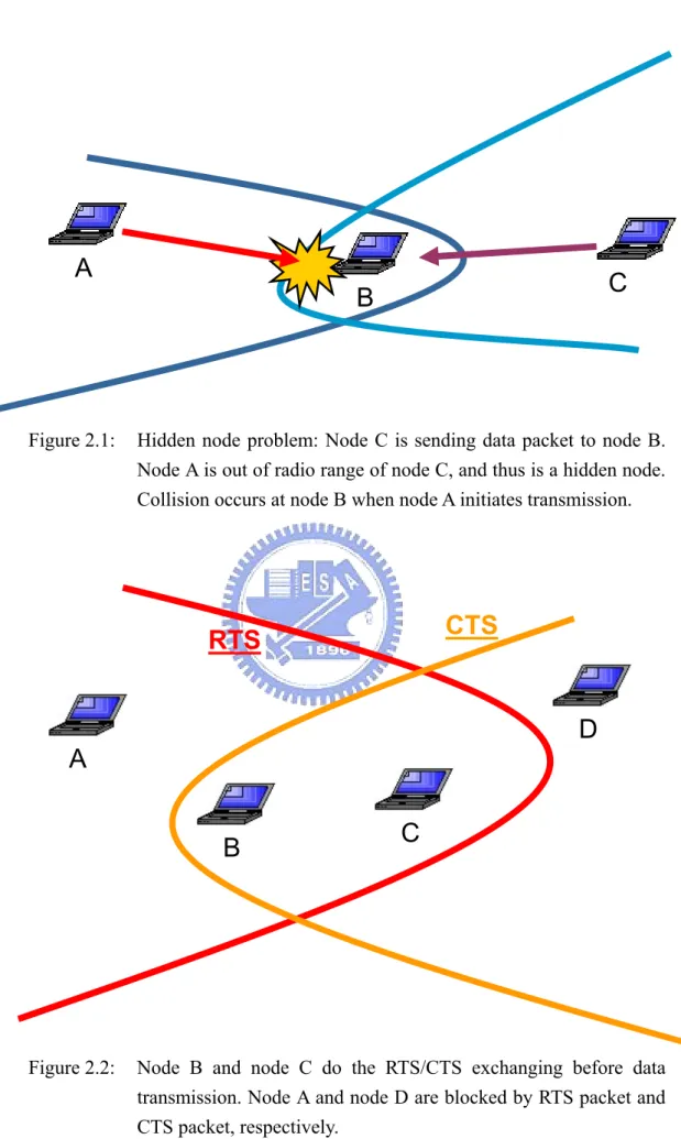
(16) carrier sense multiple access (CSMA) mechanism. The basic idea of CSMA is to reserve the radio channel for the source of a certain on-going transmission by carrier sensing. Any station wishing to transmit must sense the medium first. If some other nodes are already transmitting, the node sets a random timer and then waits for this period of time to try again. On the other hand, if the medium is currently idle, the node begins its transmission. However, the simple CSMA mechanism is susceptible to the hidden node problem, especially in wireless ad hoc networks. We begin our discussion by giving a specific description of hidden node problem.. 2.1.1 Hidden Node Problem In a wireless ad hoc network, a node can communicate with every other node in a certain range directly or use other nodes as relays. Due to lack of fixed infrastructure, it is hard for a node to be aware of other on-going transmissions. Hidden nodes are those out of range of other nodes or a collection of nodes. Thus if some neighbor nodes are already transmitting, a hidden node could send out a signal unintentionally at the same time. The signal from the hidden node collides with the transmitting signal at the receiving end and information will be lost. As depicted in Fig. 2.1, node A is out of the transmission range of node C. If node C is transmitting signal to node B, node A will not know that node B is receiving signal from node C. In the meanwhile, collision could occur at node B if node A decides to send out signal. In this case, node A is known as a hidden node. As mentioned before, hidden nodes can cause costly packet collisions and significantly reduce network performance. When a collision of data packet occurs, the data packet will be discarded, and the system must waste time on retransmissions. Therefore, many MAC protocols have been proposed to eliminate the hidden node problem. 5.

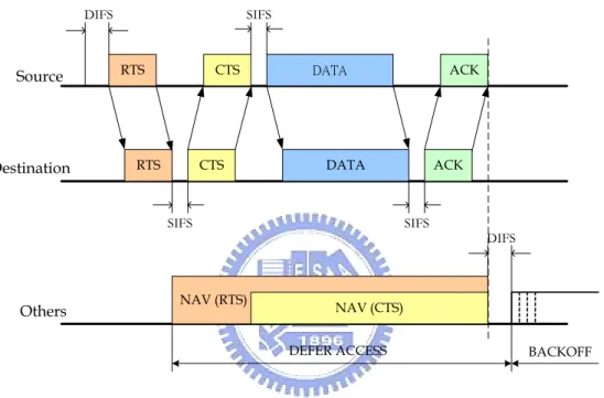
(17) 2.1.2 RTS/CTS Exchanging Mechanism In order to solve the hidden node problem, and thus achieve high throughput, a mechanism known as RTS/CTS exchanging is widely used. The RTS/CTS exchanging mechanism was initially proposed in a protocol called multiple-access with collision avoidance (MACA) [15]. A node wishing to send a data packet must firstly broadcast a request-to-send (RTS) control packet which contains the length of the data packet that will be sent. After receiving the RTS packet, the receiver responses by sending out a clear-to-send (CTS) control packet which also contains the length of the upcoming data packet. According to the data length information, any node hearing either RTS or CTS packet must set a timer to record the end of upcoming data transmission. Thus all the neighbors of the transmitting end and the receiving end will be informed about the data transmission by RTS and CTS control packets respectively. These nodes remain silent until the data transmission is completed, and therefore collisions are avoided. As shown in Fig. 2.2, node B wants to communicate with node C. Node B first sends out an RTS control packet and waits for response from node C. At the same time, node A is blocked by this RTS packet and remains silent until the end of the following data transmission. Upon receiving the RTS packet, node C sends out a CTS packet to show that it is ready for receiving data from node B. Node D also receives this CTS packet and will not send out any signal. After exchanging RTS/CTS packets, node B can start transmit data packet to node C without been interfered. This example clearly shows how the hidden node problem is eliminated by RTS/CTS exchanging mechanism, and thus collisions are avoided. Via this control packet exchanging process, all the hidden nodes won’t transmit during the period of data transmission, and the effect of hidden node problem is eliminated.. 6.

(18) However, in an ad hoc network with heavy load, there could be lots of nodes wishing to transmit data packets at the same time. This could result in the flood of RTS packets, and the flooded control packets could prohibit a large number of nodes from transmitting any packet. Consequently, the throughput of the network goes to zero as the load increases. Before giving a further description of this problem, the most widely used MAC protocol, IEEE 802.11 MAC protocol, will be introduced in the following section.. 2.1.3 IEEE 802.11 DCF protocol The IEEE 802.11 protocol covers the MAC and physical (PHY) layer. The MAC layer defines two different access methods, the distributed coordination function (DCF) and point coordination function (PCF). Since the PCF cannot be used in ad hoc networks, the following discussion will focus on the DCF protocol. IEEE 802.11 DCF protocol is basically a carrier sense multiple access with collision avoidance mechanism which is implemented by RTS/CTS exchanging. All other nodes receiving either the RTS or CTS packet set their virtual carrier sensing indicator, called a network allocation vector (NAV). The NAV is a counter counts down to zero at a constant rate, which is updated according to the duration field in the control packet. Before the NAV counts down to zero, the virtual carrier is sensed busy. Thus the area covered by the transmission range of the sender and the receiver is reserved for data transmission. In addition to the RTS/CTS packets, IEEE 802.11 DCF protocol requires an acknowledgment (ACK) packet transmitted by the receiver after the successful reception of data packet. The sender ascertains the success of data transmission by receiving the ACK packet. If no ACK packet is received, data retransmission can be initiated immediately. 7.

(19) IEEE 802.11 DCF protocol also employs a congestion control mechanism based on random backoff. When a node has data to transmit, it detects the wireless medium first. If the medium has been idle for more than a time interval called distributed inter frame space (DIFS), this node can transmit the data packet immediately. Otherwise, it waits until the medium becomes idle, and then defers for another DIFS interval. If the medium remains idle after this DIFS interval, the random backoff mechanism is started. Without the backoff mechanism, collisions may occur just at the moment because there may be more than one node waiting for the medium to become free. The node sets a backoff time that is randomly selected from interval [0 CW], where CW is the contention window value maintained in every node. At the first transmission attempt, CW is set as CWmin, and it is doubled at each retransmission up to CWmax. Once CW is set to CWmax, it remains at the value of CWmax until it is reset. The backoff timer counts down as the channel is sensed idle, pauses during data transmission, and reactivates when the medium is sensed idle again. When the backoff timer expires for more than a DIFS and the medium is still idle, the node starts transmission. If data is transmitted successfully, or maximum retry limit is reached, CW will be reset to CWmin. Fig. 2.3 shows a complete packet exchanging timing diagram of an IEEE 802.11-based wireless ad hoc network, where SIFS stands for short inter frame space. SIFS is the smallest time interval defined in the IEEE 802.11 MAC protocol. After a SIFS, only acknowledgements, CTS or data frames may be sent. At the end of a defer process, every node starts a backoff process to avoid collision at this very moment. As mentioned before, the RTS/CTS exchanging mechanism could result in poor throughput performance, especially in heavy load networks. The following section will give a thorough explanation of this RTS/CTS-induced congestion problem.. 8.

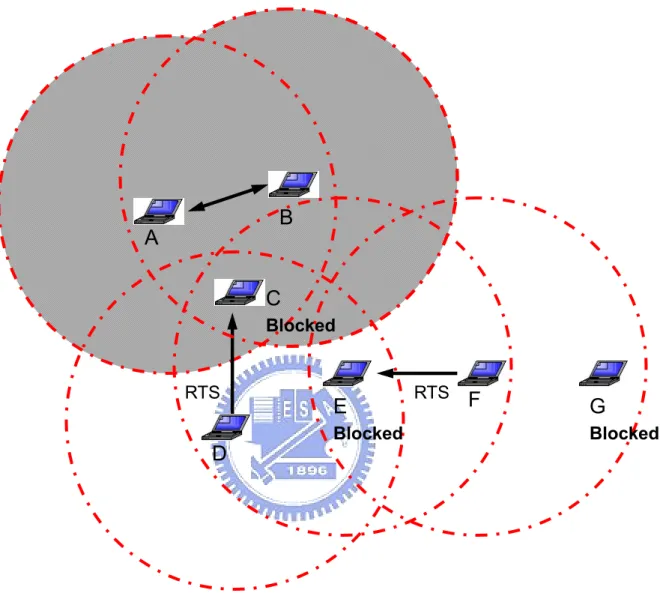
(20) 2.2. Blocking Problem. In the RTS/CTS exchanging mechanism, any node receiving either an RTS or CTS packet will be blocked for a certain period of time to ensure not to interfere with on-going transmissions. Since nodes in an ad hoc network share a single transmission channel, only one node is allowed to transmit at any time within the range of a receiver, and all the other nodes may be blocked. As for the neighbors of a blocked node, these nodes will not be aware of the fact that this node is blocked. Therefore, communication with the blocked node may still be initiated by its neighbors. In this situation, the sender sends out an RTS packet and waits for response. However, the blocked destination will not respond to this RTS packet. Since the sender does not get any response to its RTS packet, it enters into an exponential backoff mode. Furthermore, this RTS packet forces every other node that receives it to inhibit any transmission even though the blocked destination does not respond. Without a CTS response, data transmission will not be ignited. It’s a waste of medium that stations been inhibited from transmitting while no data transmission takes place actually. Fig. 2.4 explains the problem. In this figure, data packets are transmitting between node A and node B, and node C is blocked by the RTS/CTS packets from nodes A and B. In the period that node C is blocked, node D sends out an RTS packet to node C and won’t get CTS response back. Meanwhile, node E is blocked due to the RTS packet from node D. However, node E is unnecessarily blocked because it is out of the transmission range of nodes A and B. This blocking situation could propagate through the network and result in a severe problem that the throughput of the network goes to zero. If node F sends an RTS packet to node E while node E is blocked, not only node F enters into backoff mode, but also node G is unnecessarily blocked due to the RTS packet from node F. Only nodes in the gray area are required. 9.

(21) to be blocked. However, node E and node G are blocked as well. As for node D and node F, they are forced to enter backoff mode. Neither nodes in backoff mode nor nodes been blocked can transmit data, which wastes lots of radio resource. This is how blocking problem propagates and it may affect network performance severely as the load increases. From this example, we clearly show how the RTS/CTS-induced blocking problem affects the network performance. The most significant drawback is the poor throughput performance. As the load of network increases, more RTS packets are sent out, and thus more nodes are blocked. Since no node transmits data, the throughput is drastically reduced.. 2.3. Summary. In a wireless ad hoc network, a single transmission channel is shared by all of the stations. The main function of MAC layer is to manage the use of the shared medium. IEEE 802.11 MAC protocol is the most widely used protocol in the current implementation of wireless ad hoc network. This protocol is basically based on the CSMA protocol. In order to solve the hidden node problem, IEEE 802.11 MAC protocol also exploits the RTS/CTS exchanging mechanism. The RTS/CTS exchanging mechanism is widely used in wireless ad hoc networks to avoid collisions caused by hidden nodes. Any node that receives an RTS or CTS packet inhibits itself from transmitting. Therefore, data transmission can be completed without the occurrence of collision. However, the RTS/CTS exchanging mechanism could lead to blocking problem where a node could be blocked even though there is no nearby node transmitting. Moreover, the blocking problem may propagate through the network, and the throughput goes down as the load increases. From a network point of view, the 10.

(22) blocking problem reveals the tricky point of MAC functionality. On the one hand, MAC protocols must manage the shared medium to ensure successful data transmission, but on the other hand the medium reservation policy induces congestion in the network, like the blocking problem. Directional antennas have been suggested to be used in wireless ad hoc networks to reduce interference outside the intended direction, which increases spatial reuse of the transmission medium. However, from the previous sections we know that the throughput reduction results from the limitation of medium reservation. Features of directional antenna cannot be exploited without MAC protocol modification. In the following chapters, we will present ways to fully take the advantage of directional antennas.. 11.

(23) A. C. B. Figure 2.1:. Hidden node problem: Node C is sending data packet to node B. Node A is out of radio range of node C, and thus is a hidden node. Collision occurs at node B when node A initiates transmission.. CTS. RTS. D A C. B. Figure 2.2:. Node B and node C do the RTS/CTS exchanging before data transmission. Node A and node D are blocked by RTS packet and CTS packet, respectively.. 12.

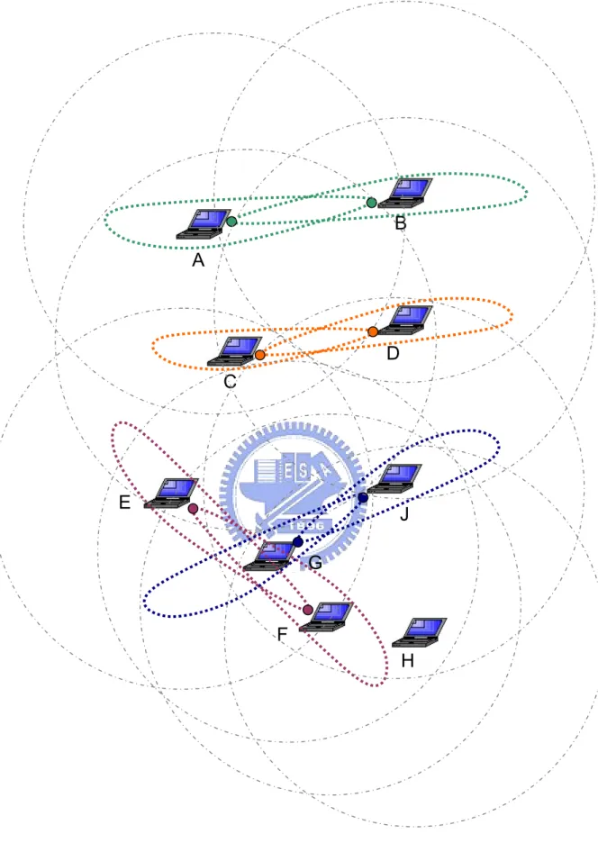
(24) DIFS. Source. Destination. SIFS. RTS. CTS. RTS. CTS. DATA. SIFS. Others. ACK. SIFS. NAV (RTS). DIFS. NAV (CTS) DEFER ACCESS. Figure 2.3:. ACK. DATA. BACKOFF. Packet transmission timing based on IEEE 802.11 MAC protocol.. 13.

(25) B. A. C Blocked. RTS. E Blocked. D. Figure 2.4:. RTS. F. G Blocked. Blocking problem: Node A and node B are transmitting data packets. Only nodes in the gray area are required to be blocked. Node E and node G are unnecessarily blocked. This figure also shows how blocking problem propagates.. 14.

(26) Chapter 3 Performance Enhancement via Directional Antennas Directional antennas offer tremendous potential for improving the performance of wireless communication systems. Continuing reductions in the cost and size of antenna arrays make it feasible for wireless mobile ad hoc networks. By using directional antennas, radio interference can be reduced effectively, thereby improving the utilization of wireless medium. With directional antennas, simultaneous data transmissions of two or more pairs of nodes located in each other’s vicinity may be allowed. However, we have shown that the throughput reduction results from the medium reservation policy in MAC protocol. Therefore the merits of directional antennas may not be fully exploited without the modification of upper layer protocols. In this chapter, we present an integrated solution to utilize the advantages of directional antennas.. 3.1. System Architecture. From the previous chapter, we know that the throughput of a wireless ad hoc network could go to zero as the traffic load increases. The goal is to utilize the 15.

(27) features of directional antennas and diminish this situation. Fig. 3.1 illustrates a network situation where network capacity is improved by using directional antennas. Node C is allowed to initiate data transmission to node D while nodes A and B are transmitting. Moreover, although node G is located in the middle of nodes E and F, data transmission between nodes G and J will not interfere with nodes E and F. However, transmission between nodes G and H is not allowed, because node G is blocked in the direction of data transmission between nodes E and F. In normal situations where nodes are equipped with omni-directional antennas, most of these nodes are blocked. Data transmission between these nodes must take turns by contention. At most two sessions are allowed to be held simultaneously. In the following discussion, the main idea is to share the knowledge of the wireless medium at the PHY layer with higher layers. In standard wireless ad hoc networks, omni-directional antennas are utilized at the PHY layer, which provides only information about received power. A more useful information, direction of arrival (DOA) can be gained via the use of directional antennas. The DOA information will be shared with higher layers. From the previous chapter, we know that the fundamental resolution to blocking problem is to modify the MAC protocol. The MAC layer protocol should not block all the other neighbors in all directions. Since directional antennas can focus energy in an intended direction, spatial reuse can be achieved. With DOA information available, nodes can be aware of directions of on-going transmissions. As a result, data transmission may be initiated on the premise that no on-going transmissions will be interfered. In order to fully exploit the advantages of directional antennas, the DOA information can be further utilized at the network layer. Since directional antennas have the ability to reduce interference in a certain range of angle, our goal is to find a routing strategy to discover a path along which the packet delivery experiences the least interference. The DOA 16.

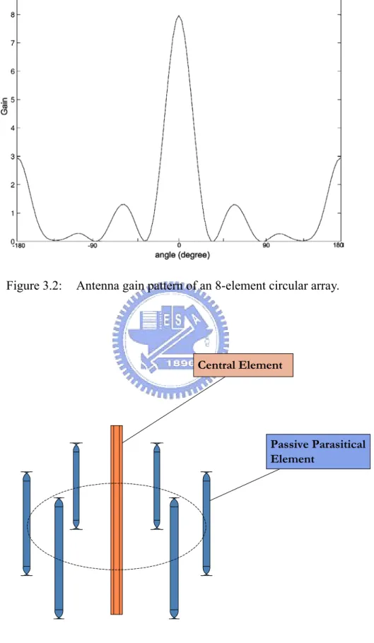
(28) information helps a node to identify the relative directions of its neighbors and the crowd level in all directions. A next hop which has fewer neighbors is preferred in our routing strategy. In this case, packets can be led through a sparsely populated area, and thus experience less interference.. 3.2. Layer 1:. Directional Antennas. Wireless ad hoc networks are conventionally equipped with omni-directional antennas. However, the technology of directional antennas for wireless mobile communication has received enormous interest in recent years. In this section, we present the implementation of directional antennas at the PHY layer.. 3.2.1 Features of Directional Antennas Directional antennas have the ability to concentrate the radiation towards the intended direction of transmission or reception. Individual elements on a directional antenna transmit signals omni-directionally, and these signals interfere with each other constructively or destructively. As a result, signal strength increases in one or more directions and eliminates in the others. Consequently, the amount of radiated power to the destined node is reduced, which can largely improve the energy efficiency. However, in the case of omni-directional antenna, the transmitted power radiates equally well in all directions and only a small percentage of power reaches the destined node. Moreover, because directional antennas have a lower gain outside the intended direction, interference can be minimized. Fig. 3.2 shows an example of beam pattern steered by an 8-element circular antenna array [16]. It has a main lobe. 17.

(29) with about 60° width and gain of 8. The radiated power is concentrated in the range from -30° to 30°, and is suppressed outside the range. In addition to the main lobe, there are also several side lobes which represent the loss of energy. With more elements on a directional antenna, the increased signal strength in the intended direction can be larger, and the control over beamwidth and direction can be more effectively. The communication area can be extended via the use of directional antennas, and the communication link can benefit more by beamforming at both transmitter and receiver.. 3.2.2 Antenna Model Most studies on wireless ad hoc networks with directional antennas have assumed the use of a small, low-cost adaptive antenna which is known as electronically steerable passive array radiator (ESPAR) antenna [17]. As shown in Fig. 3.3, the (M+1)-element ESPAR antenna consists of one center element connected to the main radiator and M surrounded passive parasitical elements in a circle. The main radiator exhibits an omni-directional radiation pattern. Each passive parasitical element is loaded with a variable reactor. The antenna pattern is formed according to the bias voltage on the reactors, and thus the reactance values. The ESPAR antenna is capable of forming either omni-pattern or sector pattern. For omni-pattern forming, the bias voltage on each reactor is set equally on condition that the received power is maximized [18]. For sector pattern forming, an optimized set of bias voltage on reactors is obtained such that the received signal power is maximized in the direction of the source. In the following discussion, the antenna system on each node is assumed to be capable of operating in two modes; omni-mode and directional mode. Both the omni 18.

(30) and the directional modes can be used to transmit or receive signals. In omni-mode, a node is capable of receiving or transmitting in all directions with a constant gain. A node stays in omni-mode while idle. In directional mode, a node can point its antenna beam towards an intended direction with a gain which is typically larger than that in omni-mode. Consequently, a node in directional mode has a greater transmission range than in omni-mode. The direction in which the main lobe should be steered for a given transmission is specified to the antenna by the upper layer protocol. When a node is in the omni-directional receiving mode, it is susceptible to interference from all directions. Only when the node has formed a beam to a specific direction, it can avoid the interference from other directions.. 3.3. Layer 2: Medium Access Control (MAC). Current MAC protocols, such as IEEE 802.11 standard, do not benefit when using directional antennas, because these protocols have been designed for omni-directional antennas. To best utilize directional antennas, a suitable MAC protocol must be well designed. The use of RTS/CTS exchanging mechanism is optional in the standard, and is assumed to be used in the following sections. The basic idea of directional MAC (DMAC) protocol is to block only those nodes located within the direction of upcoming data transmission. An intuitive way to achieve this goal is to transmit RTS/CTS packets directionally, which can thus largely reduce the number of blocked nodes. Furthermore, those nodes which received RTS/CTS packets are not blocked in all directions. Through the adoption of directional network allocation vector (DNAV) [19], these nodes can initiate data transmissions in some other directions. In the following, a DMAC protocol based on directional virtual carrier sensing (DVCS) [20] will be introduced. 19.

(31) 3.3.1 Neighbor Node Location Identification In order to steer the antenna beam to an accurate direction in its next hop and send out RTS/CTS packets directionally, the sender needs to know the relative locations of its neighbors. Some related works on DMAC protocol assume that the physical location information may be obtained by using the global positioning system (GPS), ultrasound, or multiple orthogonal channels for control packet transmission. However, these additional resource requirements could make the protocol impractical and unrealistic. For nodes equipped with directional antennas, neighbor node locations can be obtained by direction of arrival estimation techniques. Each node caches estimated DOAs from neighbor nodes when it hears any signal, regardless of whether the signal is sent to the node. In a complex environment where lots of scattering, reflection and diffraction could be induced, the result of DOA estimation may not match the physical relative direction which could be obtained by external devices such as GPS. However, the DOA information based on signal strength evaluation may be much more practical than physical location information. In other words, the DOA is the most effective direction to reach the transmitter with the minimum path loss. The DOA information is updated every time the node receives a new signal from the same neighbor. With DOA information available, RTS/CTS packets can be transmitted in an accurate direction. Therefore, only those nodes located within the direction of upcoming data transmission will be blocked. The DOA caching mechanism is implemented at routing layer and will be introduced in Section 3.4.2.1.. 20.

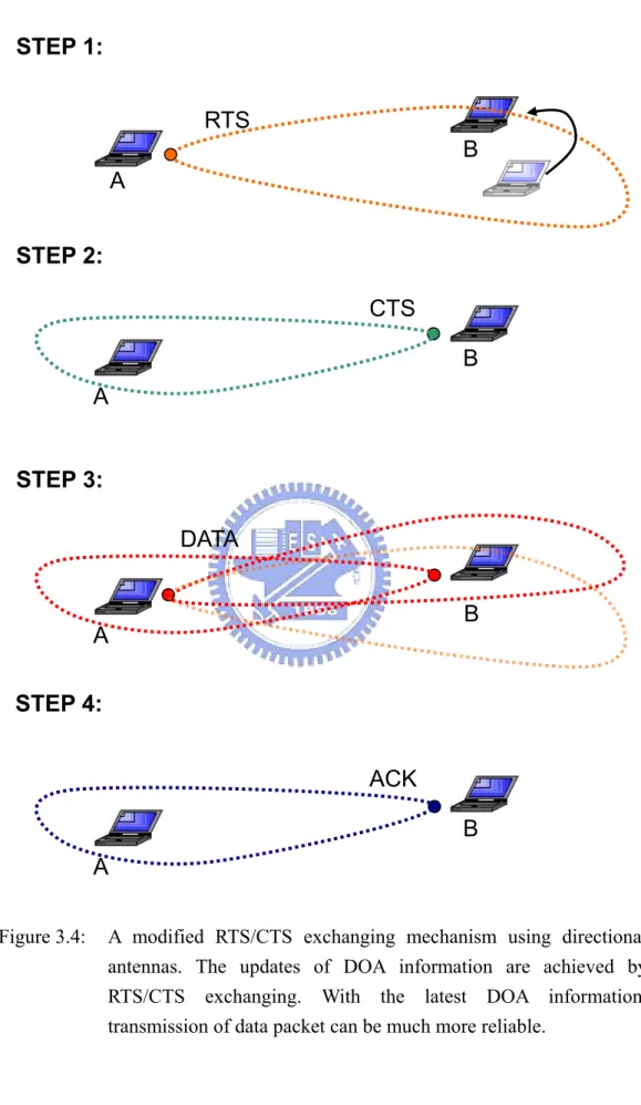
(32) 3.3.2 Modification of RTS/CTS Exchanging Mechanism This DMAC protocol is an enhancement to the IEEE 802.11 MAC protocol. As mentioned before, two modes of antenna operation are available; omni-directional mode and directional mode. A node listens to the channel omni-directionally when idle. In the DMAC scheme, the RTS, CTS, DATA, and ACK packets are sent directionally. Firstly, as in the IEEE 802.11 protocol, the sender sends out an RTS packet prior to data transmission. The RTS packet is sent directionally to the receiver according to the DOA information. When the receiver receives this RTS packet, it not only updates the DOA information, but also adapts its beam pattern to maximize the received power and locks the pattern for the CTS transmission. Once the sender receives the CTS packet, it updates the DOA information and adapts its beam pattern for the data transmission as well. This beam pattern adaptation process provides a more reliable data transmission. During the data transmission, beam patterns are locked toward each other for both transmission and reception, and are unlocked after the completion of ACK packet transmission. These locked patterns maximize the signal power at the receiver as long as the channel condition remains the same. Since the period from CTS through ACK transmission is for only a short period of time, the channel response may be assumed to be stable. Fig. 3.4 shows the steps of beam locking and unlocking. Assume that node A has data to be sent to node B. At the first step, node A transmits an RTS packet directionally toward node B according to the last updated DOA from node B. Although this RTS packet may not be sent in an accurate direction due to node movements, the direction of the upcoming data transmission can be corrected in the following steps. Upon receiving the RTS packet, node B updates its DOA information and locks its beam pattern to this newly derived direction for CTS packet. 21.

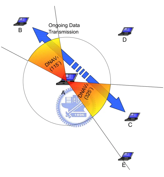
(33) transmission. At the second step, node B sends out a CTS packet toward node A. Node A updates its DOA information and locks its beam pattern to node B as well. At the third step, node A starts to transmit data packet. These locked beam patterns provide reliable data transmission at both sides. Eventually, data transmission is completed with an ACK packet replied from node B directionally.. 3.3.3 Directional Network Allocation Vector (DNAV) The value of network allocation vector indicates the duration of the ongoing transmission in the vicinity, and the node must reserve the channel for those acting nodes by deferring its own transmission. Directional NAV is an enhancement of NAV, which reserves the channel only in a certain range of directions. The design of DNAV is to release the medium which is not necessarily reserved, and thus spatial reuse can be achieved. If a node receives an RTS or a CTS packet from its neighbors, a DNAV is set. Each DNAV is tagged with two important values; the direction where the control packet comes from and the duration of the corresponding data transmission. A node cannot transmit any signals whose direction is in the range of unexpired DNAVs. Another important factor is the width of DNAV, which is based on the beamwidth formed by the directional antennas. The DNAV width of a node must be larger than the beamwidth. Assume that the width of DNAV is 2w degrees and the beamwidth is 2b degrees. For a node to transmit safely, it must refer to its DNAV table and the difference between the transmitting direction and all the DNAVs must exceed (w+b) degrees. In other words, the antenna beam intended to a certain direction must not overlap with any unexpired DNAVs. Fig. 3.5 shows a simple example where spatial reuse is achieved. Node B has data to be sent to node C, and data transmission is initiated 22.

(34) after RTS/CTS exchanging. Node A received RTS and CTS packets from nodes B and C, respectively. Two DNAVs with 60° width are set upon the reception of these control packets. The numbers in the parentheses represent the relative angles between node A and these two active nodes. If node A has a packet to be sent to node E or node D, it must refer to its DNAV table to check if there is any transmission ongoing in the corresponding direction. Node A cannot transmit any signal to node E until the expiration of DNAV2 which was set upon the reception of the CTS packet from node C. However, transmission to node D is not deferred by any DNAV, and can be ignited. As mentioned in Section 3.3.1, the DOA is always the most effective direction towards the transmitter with the minimum path loss. This also implies that transmissions towards the DOA of the transmitter could cause the most interference. Therefore, the most effective way to avoid collisions is to set DNAV according to the DOA even the signal DOA does not match where the transmitter is physically located. The width of the DNAV can also be adjusted for the control of aggressiveness of a transmitter. A DNAV with a narrower width makes more directions available for transmission, and thus makes the transmitter more aggressive. To best exploit the advantages of directional antennas, the routing protocols should be modified as well. The relative direction information of neighbor nodes can be further utilized. With DOA information available, a path from the source to the destination which may experience less interference can be determined. In the following section, we introduce the basic concepts of routing protocols in ad hoc networks, and achieve our goal by modifying a well-known routing protocol, the DSDV routing protocol.. 23.

(35) 3.4. Layer 3:. Routing. A wireless ad hoc network is a collection of mobile nodes that are free to move arbitrarily in a certain area where interconnections between nodes could change continuously. Moreover, in a wireless ad hoc network, a node can communicate with every other node in a certain range directly or use other nodes as relays. Due to lack of infrastructure, nodes themselves function as routers which discover and maintain routes to other nodes in the network. Discovering a route is to form a path from a source node to a destination node by selecting nodes in the network as relays. And maintaining a route is to take actions to reconstruct a broken route when one of the relays on the route is no longer available. Without an effective construction of routes, packets cannot be delivered reliably from one node to another, especially in a fast changing topology. The design of efficient routing protocols is the central challenge in such dynamic wireless networks. In order to fully exploit the advantages of directional antennas, we want to find a solution to explore a path which experiences the least interference. Intuitively, relaying packets through a crowded area could suffer severe interference and most of the nodes in this area could be blocked as well. If packets can be led through a sparsely populated area, packets experience less interference, and thus the transmission can be much more reliable. Therefore, our goal is to establish a routing mechanism which can discover a sparse path to dodge crowded area. Before proceeding with the discussion of our proposed routing protocol, the classification of current routing protocols will be introduced in the following section.. 24.

(36) 3.4.1 Classification of Current Routing Protocols There have been several routing protocols proposed for wireless ad hoc networks. Depending on when the route is computed, these routing protocols may be categorized as: table-driven routing and on-demand routing protocols [21]. Table-driven routing protocols are also called proactive routing or pre-computed routing protocols. As implied by the name, table-driven routing protocols attempt to maintain a table which consists of up-to-date routing information from each node to every other node in the network. In order to maintain a consistent network view, updates of routing information are propagated throughout the network periodically or whenever the link state of the network changes. The advantage of table-driven routing protocols is that a route to the destination is already available when a source wants to send packets to a certain node in the network. However, the propagation of routing information could result in flooding of update packets, which consumes a lot of the wireless network bandwidth. Destination sequence distance vector (DSDV) [3], clusterhead gateway switching routing (CGSR) [4], wireless routing protocol (WRP) [5], global state routing (GSR) [6], and fisheye state routing (FSR) [7] are examples of table-driven routing. On-demand routing protocols is also called reactive routing protocols. In this method, routes are created only when they are needed. In other words, the route may not exist in advance and it is computed just before the packet is sent. When a source needs a route to send packets to a destination, it initiates a route discovery process within the network. This process is completed once a route is found, and the route will be maintained by a route maintenance procedure which includes the detecting and rebuilding of a broken route. The major advantage of on-demand routing protocols is that the precious bandwidth of wireless ad hoc networks is greatly saved.. 25.

(37) The bandwidth consumption due to the exchange of routing information is limited because only those routes that are needed will be maintained. However, the source node must wait until such a route can be discovered. Dynamic source routing (DSR) [8], ad hoc on-demand distance vector (AODV) [9], temporally ordered routing algorithm (TORA) [10], dynamic source tracing (DST) [11], associativity based routing (ABR) [12], and signal stability-based adaptive (SSA) [13] are examples of on-demand routing. Furthermore, hybrid methods make use of both to come up with a more efficient one which minimizes the overhead incurred during route discovery and maintenance. Zone routing protocol (ZRP) [14] is an example of hybrid methods.. 3.4.2 Modification of DSDV Routing Protocol In order to establish a routing mechanism which lead packets through a sparsely populated area, routing protocols must be redesigned for this purpose. The DSDV routing protocol is a well-designed routing protocol with completed routing functionality. To lead packets along a sparse path, we propose some modifications to this routing protocol. The DSDV routing protocol described in [3] is a table-driven routing algorithm. In distance vector routing algorithms, every node maintains for each destination a set of distance vectors, each of which includes destination ID, next hop, distance, and so on. In order to keep the distance estimates up-to-date, each node exchanges distance vectors with its neighbors periodically. When a node receives distance vectors from its neighbors, it updates its distance vectors and the shortest distance to every other node is computed. By combining the next hop of nodes on the path from the source to the destination, a route with the shortest distance is completed in a distributed manner. The distance vector algorithm 26.

(38) described above is the classical distributed Bellman-Ford (DBF) algorithm [22]. A significant problem with the DBF algorithm is slow convergence. A node could take a very long time to build a path to a certain destination, especially after significant changes in the network topology. Another major performance problem with DBF algorithm is that the algorithm could cause routing loops. The primary cause of the routing loops is that nodes choose their next hops in a completely distributed fashion based on information which can possibly be stale, and therefore incorrect. One approach to the routing loop problem is to tag each routing table entry with a sequence number so that nodes can quickly distinguish stale routes from the new ones and thus avoid formation of routing loops. In the DSDV routing protocol, each node must maintain a routing table containing the next hop information for all of the possible destinations within the network. Each entry of the routing table is tagged with a sequence number assigned by the destination. As mentioned before, the sequence numbers enable the mobile nodes to distinguish stale routes from new ones, which can avoid the formation of routing loops. Update packets of routing table are periodically transmitted throughout the network to maintain table consistency. An entry with a newer sequence number is always preferred. As for those entries with the same sequence number, the one with a smaller hop count is chosen as the next hop. In other words, DSDV selects the shortest path based on the number of hops to the destination. Routing functionality is completed by exchanging routing table information throughout the network. To alleviate the potentially large amount of bandwidth required by update packets, two types of route update are defined. The first is known as a full dump which carries all the available routing information. The other one is called an incremental. An incremental routing update carries information which has changed since the last full dump. The full dump routing update can be transmitted relatively infrequently when 27.

(39) mobile nodes move slowly. Routing information exchanging can be completed by merely incremental routing updates. When movement becomes frequent, and the size of an incremental routing update increases, a full dump can be scheduled. After a full dump broadcast, the size of the following incremental routing update will be smaller. By employing these two types of update packets, the network traffic can be largely reduced. Detailed description of our proposed modification to the DSDV routing protocol is introduced in the following sections. The DOA information from the PHY layer is utilized here to determine the neighbor distribution in each direction. A neighborhood table records the relative directions to each reachable neighbor of a node, and thus the crowd level in a certain direction can be computed.. 3.4.2.1. Route Discovery. As in the DSDV routing protocol, our proposed modification requires each mobile node to maintain a routing table which lists all the possible destinations within the network. As shown in Table. 3.1, each entry is tagged with some important routing information such as a sequence number, the metric and the next hop to each destination, and the install time of each entry. The sequence number, as mentioned before, provides a judgment on the freshness of a route. Every time a destination node advertises its routing table, the corresponding sequence number is increased. Upon receiving the routing information, a route with a more recent sequence number is always preferred. For those candidates with the same sequence number, a route with the smallest metric is selected, and the corresponding node is chosen as the next hop. In a multi-hop environment, the next hop succeeds the data packets and relays forward the destination. The metric represents the crowd level of each route all the 28.

(40) way to the destination. The definition and calculation of the crowd level will be discussed later. The install time field indicates when the entry is installed in the routing table. Examining the install time of each route helps to determine when to delete stale routes. In fact, not all of the information in the routing table is exchanged through the network. As shown in Table. 3.2, update packets contains only information about reachable destinations and the corresponding metrics and sequence numbers. In addition to the routing table, a neighborhood table is maintained in each mobile node. As shown in Table. 3.3, a neighborhood table lists all the reachable neighbors and the corresponding directions. Each entry in the neighborhood table is also tagged with the install time as in routing tables. Every time a node hears a signal from one of its adjacent nodes, the DOA of this signal is estimated at the PHY layer. Since the signal can be received by this node, the sender of the signal represents a reachable neighbor of this node. If this neighbor is never heard before, it is added into the neighborhood table along with the DOA. If this neighbor is already recorded in the neighborhood table, the DOA is updated. Therefore, a node can be aware of all its reachable neighbors and the corresponding direction to each. The neighborhood table not only helps to calculate the crowd level of a route to a certain destination, but also guides the antenna beam to the right direction. Recall that at the MAC layer, an RTS packet requires a DOA caching mechanism to be sent directionally toward an intended node. That is, when relaying a data packet, a node must check its routing table for the next hop. After making sure that it has a route to the destination, an RTS packet is sent directionally toward the next hop according to the DOA information recorded in the neighborhood table. In the following, we present a routing strategy to discover a route along which packet transmission experiences the least interference. An intuitive way to achieve 29.

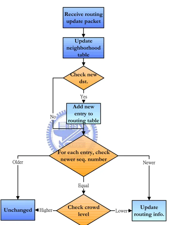
(41) this goal is to relay packets through a sparsely populated area. Firstly, the crowd level is calculated as follows. When a node receives a signal from one of its neighbors, the DOA of this signal is estimated at the PHY layer, and the neighborhood table is updated as mentioned before. If this received signal is a routing update, the node will refer to its neighborhood table for the calculation of crowd level before updating its routing table. According to the neighborhood table, the number of neighbors within a certain range of the DOA which the signal comes from can be determined. This number is regarded as the crowd level of this single hop in the corresponding direction. Secondly, the routing table is updated. The metric of each entry in the routing update is accumulated with the newly derived single-hop crowd level. As a result, the crowd level of each route in which the routing update source node is used as the next hop can be derived. An entry with a small metric represents a route along which nodes are sparsely located, and thus is preferred. The routing information update process is shown by a flow chart in Fig. 3.6. A latest sparse route can thus be derived. Fig. 3.7 is an example of sparse route selection. As shown in this figure, by the advertisement of routing update, node D is a reachable destination of node A through two different routes. Upon receiving the routing updates of nodes B and E, node A chooses one of these two nodes as the next hop to node D. According to the neighborhood table in node A, there are five neighbors in the direction of node E while there is only one neighbor in the direction of node B. Therefore, the metric in the routing updates of node E and node B are added by five and one, respectively. Similarly, as node B receives the routing update from node C, the metric is added by one. With the same sequence number, it is obvious that node A chooses node B as the next hop to reach node D. As a consequence, a sparse route is discovered. Table 3.1 shows the update of node A’s routing table. Table 3.1(a) is the routing table of node A 30.

(42) which is updated based on the routing update sent by node E at time T50. The table lists all reachable destinations and the next hop to each. The corresponding metric and sequence number of each entry are also listed for reference. To reach nodes C and D, node A relays its packets through node E. Table 3.1(b) is the routing update which was advertised by node B at time T52. This table lists all reachable destinations of node B. Each entry is tagged with a metric and a sequence number which is generated by the corresponding destination. The larger the sequence number is, the newer the route is. This routing update informs all the neighbors of node B that these destinations are reachable through node B. Upon receiving this routing update, node A refreshes its routing table which is shown in Table 3.1(c). For a certain destination, a route with a newer sequence number is preferred. Originally, to reach node C, node A has a route via node E with a sequence number of S962. After receiving node B’s routing update, the next hop is replaced with node B, and the new route has a sequence number of S964. To reach node D, node B has a route with a sequence number of S1000 which is the same as that listed in Table 3.1(a). However, the route via node B has a smaller metric and is preferred. This update of routing table completes a sparse route from node A to node D. From the previous example, we note that using node B as the next hop, node A needs three hops to reach node D while in the case of using node E as the next hop, node D is only two hops away. Since our objective is to find a sparse route, the obtained sparse route is not necessarily the shortest route. However, update information along a shorter path could arrive earlier, and is preferred for its newer sequence number. Not long after the arrival of the update along the sparse route, the former one is replaced. In order to suppress the fluctuations of the routing table, routing updates are kept for a short period of time between the arrival of the first and the arrival of the sparse route. After the arrival of the sparse route, a node can make a 31.

(43) right decision. The delay of update also helps to reduce the number of rebroadcasts of possible route entries that normally arrive with the same sequence number.. 3.4.2.2. Route Maintenance. The mobility of nodes causes broken links. The broken link may be detected by the layer-2 protocol, or it may also be inferred if no broadcasts have been received for a while from a former neighbor. Since a broken link could result in serious transmission error, a broadcast routing update containing this information should be arranged immediately. In the routing table, a broken link is described by a metric of. ∞ . Once a node detects a broken link, i.e. an unreachable next hop, it immediately assigns an ∞ metric to any route through that next hop and generates an updated sequence number. This is the only situation when the sequence number is generated by any mobile node other than the destination node. Sequence numbers defined by the originating mobile nodes are generated as even numbers, and sequence numbers generated to indicate ∞ metrics are odd numbers. Upon receiving the notification of a broken link, a node updates its routing table and continues to advertise the broken link. When a node receives an ∞ metric, and it has a later sequence number with a finite metric, it triggers a route update broadcast to disseminate the important news about that destination. In summary, the amount of overhead required for the proposed routing strategy is the extra memory for neighborhood table and the computation of crowd level. However, both the MAC and routing functionality can benefit from the establishment of neighborhood table. Furthermore, the directional antenna adopted at the PHY layer has no effect on the amount of overhead. In other words, a smaller sector size or beamwidth of a directional antenna does not result in more overhead. 32.

(44) 3.5. Summary. From the previous chapter, we know that the throughput reduction results from the medium reservation policy in MAC protocol, and the merits of directional antennas cannot be fully exploited without the modification of upper layer protocols. In this chapter, we propose an integrated refinement of MAC and routing protocols with the use of directional antennas. A node equipped with directional antennas has the ability to estimate the DOA of an incoming signal and thus can identify the relative directions of its neighbors. Before transmitting data packets, nodes exchange RTS/CTS packets directionally, therefore, only those nodes located within the direction of transmission are blocked. Moreover, if a node receives an RTS or a CTS packet from its neighbors, a DNAV is set according to the DOA of that control packet, and the duration as well. With the help of DNAV, a node is blocked only for those directions where RTS/CTS packets come from, and spatial reuse can thus be achieved. Furthermore, to fully exploit the advantages of directional antennas, we propose a routing strategy to discover a route that experiences the least interference. The DOA information helps a node to identify the relative directions of its neighbors and the crowd level in every direction. Our proposed routing strategy prefers a next hop which has fewer neighbors. Therefore, packets can be routed to the destination through a sparsely populated area. The joint design of MAC and routing protocols fully exploits the advantages of directional antennas and improves the throughput performance significantly. In the following chapter, we present some computer simulation results to verify improvements over the omni-directional approach.. 33.

(45) B A. D C. E. J G. F H. Figure 3.1:. Network capacity is improved via directional antennas. Four sessions is allowed to be held simultaneously without interfering with each other. While in the case of omni-directional communication, most nodes are blocked. 34.

(46) Figure 3.2:. Antenna gain pattern of an 8-element circular array.. Central Element. Passive Parasitical Element. Figure 3.3:. A 7-element electronically steerable passive array radiator antenna. The central element is connected to the main RF radiator. Each passive parasitical element is loaded with a variable reactor. 35.

(47) STEP 1: RTS B A STEP 2: CTS B A STEP 3: DATA B. A STEP 4: ACK. B A Figure 3.4:. A modified RTS/CTS exchanging mechanism using directional antennas. The updates of DOA information are achieved by RTS/CTS exchanging. With the latest DOA information, transmission of data packet can be much more reliable.. 36.

(48) B. Ongoing Data Transmission. D. A. DN (32 AV2 5° ). V1 A ) DN 15° (1. C. E. Figure 3.5:. Spatial reuse can be achieved by the adoption of DNAV. Two DNAVs reserve the wireless medium for nodes B and C. The blank area represents available directions for node A’s transmission.. 37.

(49) Receive routing update packet Update neighborhood table Check new dst. Yes. No. Add new entry to routing table. For each entry, check newer seq. number. Older. Newer. Equal. Unchanged. Higher. Figure 3.6:. Check crowd level. Lower. Update routing info.. Flowchart of routing information update.. 38.

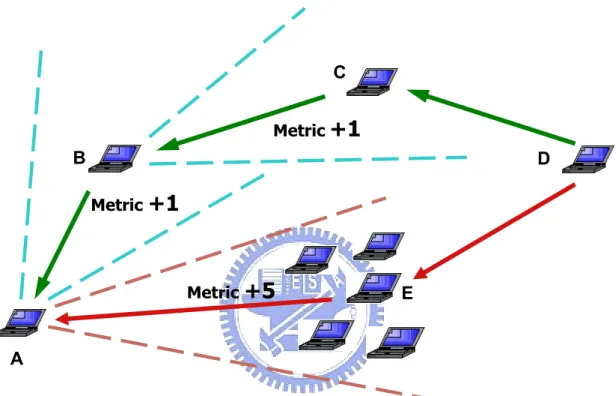
(50) C Metric +1. B. D Metric +1. Metric +5. E. A. Figure 3.7:. Two different routes are available for node A to reach node D. By the calculation of crowd level, a sparse route can be determined, and packets will not be relayed through a crowded area.. 39.

(51) Table 3.1: Destination. Metric. Routing table.. Sequence number. Table 3.2: Destination. Neighbor. Update packet.. Metric. Table 3.3:. Next hop. Sequence number. Neighborhood table.. Angle. 40. Install time. Install time.

(52) Table 3.4:. Example of routing table update. With the same sequence number, a route with a smaller metric is preferred. A sparse route from node A to node D is completed after the update of routing table.. (a) Routing table of node A after receiving the update from node E Destination. Metric. Sequence number. Next hop. Install time. A. 0. S1012. A. T46. D. 6. S1000. E. T50. C. 7. S962. E. T50. E. 5. S850. E. T50. (b) Routing update sent by node B at time T52 Destination. Metric. Sequence number. B. 0. S920. A. 1. S1012. C. 1. S964. D. 2. S1000. (c) Routing table of node A after receiving the update from node B Destination. Metric. Sequence number. Next hop. Install time. A. 0. S1012. A. T46. D. 3. S1000. B. T52. B. 1. S920. B. T52. C. 2. S964. B. T52. E. 5. S850. E. T50. 41.

(53) Chapter 4 Computer Simulations To evaluate the performance of the proposed system architecture, we use the NCTUns 1.0 network simulator [23]. As NCTUns does not support network environment with directional antennas, we implement the directional antenna module based on the system architecture described in Chapter 3. Each node in the network is assumed to have an electrically steerable directional antenna system. For simplicity, as most studies on wireless ad hoc networks using directional antennas, a flat-topped antenna pattern is used in our simulation. A flat-topped antenna pattern has a constant gain for all directions within the specified angle, and has a lower constant gain for all other directions, representing side lobes of the pattern. This beam is steered under the control of the routing protocol as discussed in Section 3.4.2. In our simulations, a directional antenna gain of 8 is assumed within a 60-degree angular region, and a lower gain of 0.2 is assumed for all other regions. The destination of each transmitting node is chosen randomly. The packet length is constant and equals to 1000 bytes. The approximate omni-transmission range is 250 meters. We use the two-ray ground propagation model as the path loss model. Each simulation run is conducted for 200 seconds, and each data point is the average of 3 simulation runs. The following sections present some simulation results that show how the capacity of wireless ad hoc networks depends on these parameters. 42.

(54) 4.1. Blocking Problem. Recall that in Chapter 2, we have shown that the RTS/CTS exchanging mechanism may lead to a congestion situation where most of the nodes in a network are unable to transmit any packets during long periods of time. As a result, the network throughput decreases with increasing traffic load instead of maintaining its peak value. In this section, we present the simulation result of the blocking problem. We use a rectangular grid arrangement of the nodes. The network consists of 25 static nodes arranged as a 5×5 square. The distance between nodes horizontally and vertically is 200 meters. Fig. 4.1 shows the simulation result of the throughput performance as the traffic load increases. The traffic load is defined as the percentage of source nodes in the network wishing to transmit data. Two different configurations of operating mode are included: directional mode and omni-mode. In the directional mode, as described in Chapter 3, each node adopts the DMAC and the modified DSDV routing protocol for directional transmission. In the omni-mode, each node transmits and receives packets omni-directionally with the standard IEEE 802.11 DCF and unmodified DSDV routing protocol. From Fig. 4.1(a), it is clear that the throughput of the network operating in the omni-mode goes to zero as the traffic load is increased, which implies that the network behaves like a congested network. While in the case of directional mode, the throughput performance is greatly improved and maintains an acceptable value under heavy traffic loading. Another important factor, the average delay of packet delivery is also improved in the operation of directional mode. Fig. 4.1(b) shows the average packet delay as the traffic load increases. The difference between these two operating modes is not significant under low loading situation. However, as the traffic load exceeds 50%, the average delay of standard omni-mode increases drastically, while in the case of directional mode, the average. 43.

(55) delay remains stable until the traffic load exceeds 80%. Also, under any load situation, operating in the directional mode yields a lower average delay. This gives an indication of the alleviation of RTS/CTS-induced congestion problem by spatial reusing.. 4.2. Effects of Mobility. The main objective of the simulations is to qualitatively analyze the capacity improvement in wireless ad hoc networks when directional antennas are used for communication. In this section, we present the simulation result of the overall system throughput. The network consists of 15 mobile nodes randomly distributed in an 800 meters ×800 meters square area, in which 5 nodes are randomly selected as source nodes wishing to send data packets. In the mobility scenario, the random waypoint model is used as the mobility model in which each node moves straight towards a randomly chosen destination at a constant speed. After the node reaches the destination, it chooses another point and moves toward the new destination without pause. Three different configurations of operating mode are included: directional mode, omni-mode, and direction mode with unmodified DSDV routing protocol. In the third configuration, the PHY and MAC layers are implemented as the directional mode, while the routing layer adopts the unmodified DSDV routing protocol. Fig. 4.2(a) shows the simulation result of the throughput performance as the moving speed of nodes in the network increases. For all the three cases, the throughput performance goes down as the mobility increases. However, it is clear that the two modes using directional antennas at the PHY layer and the corresponding DMAC have outstanding performance over the omni-mode. This indicates that the potential of spatial reuse has a significant improvement on 44.