表面聲波陀螺儀的設計

全文

(1)國立交通大學機械工程學系碩士論文. 表面聲波陀螺儀的設計. Design of Surface Acoustic Wave Gyroscope. 研究生：邱仕釧指導教授：陳宗麟. 教授. 中華民國九十四年七月.

(2) 表面聲波陀螺儀的設計 Design of Surface Acoustic Wave Gyroscope. 研究生：邱仕釧. Student：Shih-Chuan Chiu. 指導教授：陳宗麟. Advisor：Tony Chen. 國立交通大學機械工程學系碩士論文. A Thesis Submitted to Department of Mechanical Engineering College of Engineering National Chiao Tung University in Partial Fulfillment of the Requirements for the Degree of Master of Science in Mechanical Engineering July 2005 Hsinchu, Taiwan, Republic of China. 中華民國九十四年七月.

(3) 表面聲波陀螺儀的設計學生: 邱仕釧. 指導教授: 陳宗麟. 博士. 國立交通大學機械系碩士班. 摘要近年來，微機電 (MEMS) 系統的感測器越來越受到重視。由於利用是標準積體電路製造技術製得，因此通常有輕量化、微小化、功率損耗較小和低成本等優點。表面聲波陀螺儀是由表面聲波諧振器 (surface acoustic wave resonator) 和表面聲波感測器 (surface acoustic wave sensor) 所組合而成。表面聲波陀螺儀相較於目前微機電陀螺儀本身的性能的限制，具有低成本、強健性和穩定性等優點。本研究中，針對此種操作在射頻 (radio frequency) 的表面聲波陀螺儀的設計與其性能加以分析、探討。並且利用表面聲波元件其能量傳遞與粒子真實位移的轉換，來預估表面聲波陀螺儀之感測精度。. I.

(4) DESIGN OF SURFACE ACOUSTIC WAVE GYROSCOPE Student: Shih-Chuan Chiu. Advisor: Dr. Tony Chen. Department of Mechanical Engineering National Chiao Tung University. Abstract The preliminary design and performance evaluation of a radio frequency MEMS gyroscope, based on a surface acoustic wave resonator (SAWR) and a surface acoustic wave sensor (SAWS) is presented in this work. In addition, the method to convert the transmitted power into exact particle displacement is introduced to predict the sensing resolution of this MEMS gyroscope. Microelectromechanical systems (MEMS) sensors have received more attention over the last decade. They generally have the advantages of being lightweight, small in size, low power consumption and low cost, due to standard IC fabrication techniques. The gyroscopes, operated on the surface acoustic wave, are expected to have a better performance limitations over current MEMS vibratory gyroscope designs, for example, low cost, better robustness and reliability.. II.

(5) 致謝本論文得以順利完成，首先要感謝我的指導教授陳宗麟老師的指導，在老師嚴謹的治學帶領下，總是能周詳地考慮所面臨的問題，在作者產生疑惑時，一針見血地點明癥結點，並且加以指導、糾正；兩年的光陰，作者受益良多，在此致上最誠摯的感謝。同時感謝口試委員尹慶中教授、蘇育全教授對本論文給予的指導與建議，以及固控組諸位老師，對於作者課業上的指導與關懷。感謝實驗室學長紀建宇對作者研究上的指教，同學陳奕龍、黃建評、郭威廷及學弟許齡元、林志柏、高忠福的相互砥礪，使本人的課業及研究工作得以順利進行，在此一併致謝。另外感謝好友陳億珊、賴穎鋒以及大學、高中的好友們的支持與精神鼓勵，使作者的研究生活得以順利進行。最後謹將本論文獻給最親愛的母親，感謝他們多年來付出的辛勞，在她的細心呵護下，本人才有今天小小的成果，希望能與她分享今日的喜悅；以及親友的支持與鼓勵，使作者在無後顧之憂下完成學業，謹此獻上最誠摯的謝意。. III.

(6) Table of Contents Abstract (Chinese)................................................................................................. I Abstract (English) ................................................................................................II Acknowledgement.............................................................................................. III Table of Contents ............................................................................................... IV List of Figures .................................................................................................... VI Chapter 1 Introduction ................................................................................... 1 1.1. Vibratory Gyroscope .......................................................................... 1. 1.2. Surface Acoustic Wave (SAW) ......................................................... 2. 1.3. Comparison between conventional MEMS vibratory gyroscope and SAW gyroscope.................................................................................. 2. 1.4. Literature Survey................................................................................ 3. Chapter 2 Interdigital-Electrode Transducers for Surface Waves ............ 5 2.1. 2.2. 2.3. Coupling-of-Modes Theory ............................................................... 5 2.1.1. The 2×2 Reflector Matrix [G] .................................................. 6. 2.1.2. The 3×3 IDT Matrix [T] ........................................................... 6. 2.1.3. The 2×2 Acoustic Spacing [D] ................................................. 9. Crossed-Field Model ........................................................................ 10 2.2.1. Electroacoustic Equivalences ................................................. 11. 2.2.2. Admittance Matrix for IDT .................................................... 11. Electromechanical Interaction.......................................................... 13. Chapter 3 Design and Simulation of SAW Gyroscope............................... 19 3.1. Surface Acoustic Wave Gyroscope.................................................. 19. 3.2. Preliminary Design of SAW Gyroscope.......................................... 20. 3.3. 3.2.1. Operating Frequency .............................................................. 20. 3.2.2. Substrate.................................................................................. 21. 3.2.3. Interdigital Transducer............................................................ 21. 3.2.4. Reflector.................................................................................. 22. 3.2.5. Spacing.................................................................................... 22. 3.2.6. Metallic Dot Array.................................................................. 22. Transformation of Coriolis force...................................................... 23 IV.

(7) 3.4. Estimation of Sensing Resolution for SAW Gyroscopes ................ 24. 3.5. Discussion ........................................................................................ 24. Chapter 4 Conclusion and Future Work..................................................... 26 4.1. Conclusion........................................................................................ 26. 4.2. Future Works .................................................................................... 26. Reference........................................................................................................... 28. V.

(8) List of Figures Fig. 1. The Coriolis effect............................................................................ 31. Fig.2a. Displacement of particles on the surface of half space due to the Rayleigh wave .................................................................................. 32. Fig. 2b. Interdigital transducer, formed by patterning electrodes on the surface of a piezoelectric crystal, for exciting surface acoustic wave: (a) SAW electrical potential, (b) plan view, (c) side view ............... 32. Fig. 3. Configuration of the IDTs, the reflectors and the perturbation electrodes.......................................................................................... 33. Fig. 4. (a) Basic elements of gyroscope: IDT, acoustic spacing and reflector. (b) Schematic representation of a SAW devices using transmission matrix ............................................................................................... 33. Fig. 5. The SAW reference planes at the ith element of a SAW reflection grating of length L............................................................................ 34. Fig. 6. Schematic representation of electrical and acoustic ports ............... 34. Fig. 7. Schematic matrix representation of a two-port SAW resonator ...... 35. Fig. 8. An instantaneous E-field direction in the crossed-field model........ 35. Fig. 9. (a) Representation of the SAW IDT as a three network, Port 1 and 2 are normally assigned to the “ acoustic” ports, while Port 3 is the electrical port. (b) In the crossed-field model, acoustic signals at Port 1 and 2 are converted to equivalent electrical transmission-line parameters ........................................................................................ 36. Fig. 10. Crossed-field model of equivalent circuit representation ................ 36. Fig. 11. (a) The ABCD matrix representation of a transmission-line section of length d, with characteristic impedance ...................................... 37. Fig. 12. Transducer composed Nt number of fingers, acoustically in cascade and electrically in parallel................................................... 38. Fig. 13. Block diagram of receiving transducer configurations. Transducer with acoustic generator at port 1 ...................................................... 38. Fig. 14. Layout of the system for the excitation of surface Rayleigh waves in a piezoelectric medium .................................................................... 39. Fig. 15. Coriolis forces acting on particles.................................................... 39. Fig. 16. Working principle of the MEMS SAW gyroscope .......................... 40. Fig. 17. Design of SAW gyroscope ............................................................... 40 VI.

(9) Fig. 18. The design of interdigital transducer ............................................... 41. Fig. 19. Result of the numbers of RIDT electrodes vs. transmitted power... 41. Fig. 20. SIDT output voltage vs. number of electrodes of SIDT .................. 42. Fig. 21. The transmitted power with different fingers of reflector of SAW resonator on two ends....................................................................... 42. Fig. 22. The sensing resolution of the proposed SAW gyroscopes with 90 fingers of sensor IDT and calculated data by Varadan et al. ........... 43. Fig. 23. The sensing resolution of the proposed SAW gyroscopes with 89 fingers of sensor IDT and calculated data by Varadan et al. ........... 43. VII.

(10) Chapter 1 Introduction. Recently, there have been increasing needs for smaller and inexpensive gyroscope (or angular rate sensors) due to the emergence of new consumer and automotive products that demand angular velocity information. Currently, the existing technologies for gyroscope including: rotating wheel gyroscopes, fiber optic gyroscopes, laser gyroscopes, vibratory gyroscope, and etc. Although, they are expensively, they have been used extensively in navigation and guidance systems. The SAW gyroscope is an MEMS device with the moderate performance. It can be made cheap and thus can have a great potential in the consumer electronics appliances in near future. The SAW gyroscope is a new technology that combines surface acoustic wave and vibratory gyroscope for the angular rate sensing, proposed by Kurosawa [8]. Many other researchers did the similar designs [10, 11, 12] and discussed their feasibility. However, none of a report stated clearly of their analysis work regarding the prediction of sensing resolution for the gyroscope. In this report, we attempted to estimate its sensing resolution by combining three analysis methods, which were well-accepted by SAW devices researchers. They are “COM theory”, “Crossed-field model” and “Electromechanical interaction”. The background knowledge for the vibratory gyroscope and surface acoustic wave is introduced below.. 1.1. Vibratory Gyroscope Angular rate sensing is typically accomplished by measuring the effect of Coriolis. acceleration on a moving body. To understand the Coriolis effect, let’s imagine a particle traveling in space with a velocity vector. ( vv ) . An observer sitting on X-axis of the XYZ. coordinate system, shown in Fig. 1, is watching this particle. If the coordinate system along. v. ( ). with the observer starts rotating around the Z-axis with an angular velocity Ω , the observer would think that the particle is changing its trajectory toward the X-axis with acceleration. v. v. equal to 2Ω × v . Since the force is proportional to the angular rate of the rotating frame, this effect has been widely used as one mean to measure the angular rate, and is the basic 1.

(11) operating principle underlying all vibratory structure gyroscopes [1]. Vibratory gyroscope mainly contains proof mass and spring. Recent advances in micro-machining technology have made the design and fabrication of MEMS vibratory gyroscopes possible. These devices are several orders of magnitude smaller than conventional mechanical gyroscope, and can be fabricated in large quantities by batch processes [2]. There are several types of MEMS gyroscope, such as: piezoelectric, piezoresistive, capacitive, acoustic wave, and optical methods.. 1.2. Surface Acoustic Wave (SAW) The stress-free boundary imposed by surface of a crystal gives rise to a unique acoustic. mode whose propagation is confined to the surface, and is therefore known as a surface-acoustic-wave (SAW). They can be classified according to different materials, boundary. conditions. and. directions. of. propagation. such. as. Rayleigh. wave,. Bleusstein-Gulyave wave, love wave, and etc. In 1887, Lord Rayleigh discovered this mode of propagation in which acoustic energy is confined very near the surface of an isotropic solid. This mode, now know as the Rayleigh wave, is of interest to seismologists because it can be used to describe earthquakes [3]. The displacement of particles near the surface due to the Rayleigh wave has an out-of-surface motion that traces an elliptical path, as shown in Fig. 2a. The Rayleigh wave can be generated at the surface of piezoelectric material and elastic material by applying a voltage to an interdigital transducer (IDT) patterned on the substrate, as shown in Fig. 2b.. 1.3. Comparison between conventional MEMS vibratory gyroscope and SAW gyroscope Due to the working principle of the vibratory gyroscopes, the vibratory gyroscopes. usually have a suspended structure to achieve vibratory motion. It is usually difficult and expensive to fabricate the suspended mechanical structures with matching resonant frequencies for the need of gyroscopes, and thus result in performance limitation for the gyroscopes sensing resolutions. Furthermore, the suspended of vibrating structure is easily subjected to the external shock and vibration, which may taper the use of gyroscopes in severe environment. In addition, to achieve high Q-factor for MEMS devices, the vacuum packing. 2.

(12) should be employed to decrease the loading from the atmosphere [5]. These constraints greatly taper the applications of MEMS gyroscopes. The SAW gyroscope can overcome those limitations since it has no suspended mechanical structure that can avoid external shock and vibration. Plus, it is a two-dimensional structure similar to the current SAW filters, as it can be fabricated by depositing electrodes on the surface of piezoelectric materials. Besides, since there is no suspended structure in SAW gyroscope, it can have high sensitivity without the need of vacuum packaging. Therefore, SAW gyroscopes have a great potential to lots of applications.. 1.4. Literature Survey It was not a new concept of using surface acoustic wave propagating on medium to. detect angular rate of an object in motion. In the early 1974, the research of surface acoustic gyro was started. In 1977, it was reported several types of simulation structures of surface acoustic wave gyro. They used aluminum alloy cylinder or fuse quartz cylinder as propagating medium for surface acoustic wave, which was excited and detected by outboard electromagnetic transducer. Besides, Forst et al. had measured real signal of SAW gyroscopes based on the design above. The operation principle of SAW gyroscopes was similar to optical gyroscopes, i.e. two surface wave propagated in opposite direction along surface of cylinder is subjected to rotation. It would produce phase difference between two surface waves, and the angular velocity is found by measured this phase difference. Due to the velocity of SAW five order smaller than light, it was predicted that the sizes of SAW gyroscopes would better than optical gyro. So far, there was no follow-up paper about this research. In 1980, B.Y. Lao [5, 7] derived theoretically the dependence of SAW velocity on the rotation rate of wave-propagating medium and it was established that, for an isotropic medium, the rotation rate was a function of Poisson’s ratio. From the relation, he proposed a new design of SAW gyroscope. It was using fuse quartz cylinder which deposited a layer of thin piezoelectric film as propagating medium. The acoustoelectric transformation for excited and detected surface acoustic wave was directly using the piezoelectric effect of material, not outboard electromagnetic transducer. According to the report, with the use of piezoelectric materials, it could increase efficiency of the transformation and greatly reduce the size of SAW gyroscope. In 1985, a new concept of SAW gyroscope was proposed [5]. It was a planar structure. 3.

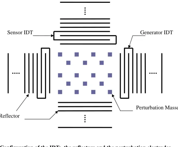
(13) The surface acoustic wave was excited by interdigital transducer on a piezoelectric material substrate. In 1998, M. Kurosawa [8] proposed a new type of SAW gyro sensor. He did the design simulations based on the equivalent circuit of the piezoelectric material. This gyro consists of generator interdigital transducer (GIDT), sensor interdigital transducer (SIDT), reflectors and perturbation mass, as shown in Fig. 3. The angular velocity of a body in motion was detected by the standing wave produced by these components. According to the report, the angular velocity could not be experimentally measured yet because the resonant frequency of RIDT and anti-resonant frequency of SIDT were not matched in experiment. In 1999, Varadan and coworkers [9, 10, 11] presented another SAW gyroscope design with a two-port resonator and sensor. The sensing resolution was 1o sec obtained in experiment. In 2002, R. C. Woods et al. [12] reported experimental trials of several SAW devices to evaluate the performance of SAW gyroscope and also made an order-of-magnitude estimate of the sensitivity. His conclusion for this device was that this device was extremely insensitive to measure the angular velocity.. 4.

(14) Chapter 2 Interdigital-Electrode Transducers for Surface Waves. Interdigital-electrode transducers were used to excite and detect the waves on the piezoelectric substrate, such that Rayleigh wave, Love wave, and etc. They play key roles in most of the SAW devices. This chapter introduces two methods which are suitable for modeling the behavior of interdigital-electrode transducers for surface wave. In the last of this chapter, we will present a study on the electromechanical interaction between interdigital-electrode transducers and a semi-infinite piezoelectric material. All of these three methods would be utilized in the design process of our SAW gyroscope.. 2.1. Coupling-of-Modes Theory The COM theory [13, 14, 15, 16, 17, 18, 19] has been extensively used since 1950s in. various problems related to optical and electromagnetism for the description of wave propagation in periodically perturbed media. It provides an efficient and highly flexible approach for modeling various kinds of SAW devices by a set of transfer matrices. In general, there are three types of the representative elements for a SAW device: IDT, spacing, and reflector, which can be described as transmission matrices [T], [D] and [G]. Depending on the configuration of a SAW devices, any number of [T], [D] and [G] matrices can be used, but their basic form remain the same. For example, the basic elements of SAW devices consist of an IDT and reflector can be modeled as shown in Fig. 4. Fig. 4(a) shows the basic elements, which has IDT, acoustic spacing and reflector. It can be represented with [ T1 ], [ D2 ], and [ G3 ], as shown as Fig. 4(b). The indexes 1－3 are just for book-keeping purpose. a and b denote complex electrical input and output signals respectively. The SAW coming in and out of each representative section is described by the complex amplitudes of forward, W + , and backward, W − . The amplitudes have dimensions of Power . In matrix form, amplitudes at an ith reference axis are ⎡Wi + ⎤ [Wi ] = ⎢ − ⎥ . ⎣Wi ⎦. (2.1). 5.

(15) Thus, any (i − 1)th SAW amplitudes coming in and out of ith section has following relation, where components of the transmission matrices are T, D and G: ⎡Wi −+1 ⎤ ⎢ − ⎥ = [T , D, G ]n ⎣Wi −1 ⎦. ⎡Wi + ⎤ ⎢ − ⎥. ⎣Wi ⎦. (2.2). 2.1.1 The 2×2 Reflector Matrix [G] Matrix [G] is a 2×2 transmission matrix applied to the SAW reflection gratings, as shown in Fig. 5. The wave amplitudes at x = －L in terms of the wave amplitudes at x = 0 yields the following transmission relation. ⎡W + ( − L ) ⎤ ⎡W + ( 0 ) ⎤ G = ⎢ − ⎥ [ ]⎢ − ⎥, W L W 0 − ( ) ( ) ⎣ ⎦ ⎣ ⎦. (2.3). where the transmission matrix [G] is. ⎛⎡ σ ⎤ j β0 L ⎛ δ − jα ⎞ + j⎜ ⎜⎢ ⎟ tanh (σ L ) ⎥ e ⎜ κ12 ⎝ κ12 ⎠ ⎦ [G ] = C ⎜ ⎣ ⎜ − je jθr tanh (σ L ) e − j β0 L ⎜ ⎝. ⎞ ⎟ ⎟ ⎟, ⎡σ ⎤ − j β0 L ⎟ ⎛ δ − jα ⎞ − j⎜ ⎢ ⎟ tanh (σ L ) ⎥ e ⎟ ⎝ κ12 ⎠ ⎣ κ12 ⎦ ⎠ je − jθr tanh (σ L ) e j β0 L. (2.4). where 1. 2 2 σ = ⎡κ12 − (δ − jα ) ⎤ ,. ⎦. (2.5). ⎛κ ⎞ C = ⎜ 12 ⎟ cosh (σ L ) , ⎝σ ⎠. (2.6). ⎣. and α is the grating attenuation constant (m-1), L is grating length (m), θ r is the reference phase, κ = κ12 is the mutual-coupling coefficient (m-1), and δ = 2π ( f − f 0 ) v0 + κ11 is the frequency-deviation (detuning) parameter from the Bragg frequency f 0 , where κ 11 is the self-coupling coefficient (m-1) related to velocity shift. ( dv v ) .. 2.1.2 The 3×3 IDT Matrix [T] The transmission matrix T of an IDT can be found by manipulating the admittance 6.

(16) matrix based on a Mason equivalent circuit model which described in detail at section 2.2. It is required to relate electrical and acoustic parameters for each IDT. The transmission matrix [T] can be equated to these by. ⎡Wi −+1 ⎤ ⎡Wi + ⎤ ⎢ −⎥ ⎢ −⎥ ⎢Wi −1 ⎥ = [T ] ⎢Wi ⎥ , ⎢ bi ⎥ ⎢ ai ⎥ ⎣ ⎦ ⎣ ⎦. (2.7). where ai and bi , respectively, denote complex electrical input and output strengths at the. ith port. Reference planes for the IDT are as shown in Fig. 6. The IDT matrix elements in Eq. (2.7) are given as [15] ⎡ t11 ⎢ [T ] = ⎢ t12 ⎢⎣ st13. where s = ( −1). Nt. −t12 t22 − st23. t13 ⎤ ⎡t t23 ⎥⎥ = ⎢ τ t33 ⎥⎦ ⎣ s. τ⎤. , t33 ⎥⎦. (2.8). is a symmetry parameter and s = 1 or s = −1 for an IDT with an even or. odd number of electrodes N t , and the elements in matrix is ⎡ ⎛ Ga ( Rs + Z e ) ⎞ jθ ⎢ s ⎜1 + ⎟e t 1 θ j + e ⎢ ⎝ ⎠ t=⎢ ⎢ s ⎛ Ga ( Rs + Z e ) ⎞ ⎜ ⎟ ⎢ ⎝ 1 + jθ e ⎠ ⎣. ⎛ G ( R + Ze ) ⎞ −s ⎜ a s ⎟ ⎝ 1 + jθ e ⎠. ⎤ ⎥ ⎥ ⎥, ⎛ Ga ( Rs + Z e ) ⎞ − jθt ⎥ s ⎜1 − ⎟e ⎥ 1 + jθ e ⎠ ⎝ ⎦. (2.9). with. θ e = (ωCT + Ba )( Rs + Z e ) ,. (2.10). θt = Nt Λδ ,. (2.11). ⎡ 2Ga Z e jθt 2 ⎤ e ⎢ ⎥ ⎢ 1 + jθ e ⎥ τ =⎢ ⎥, jθt 2 G Z a e ⎢ e 2 e − jθt ⎥ ⎢⎣ 1 + jθ e ⎥⎦. (2.12). and. ⎡. 2Ga Z e jθt 2 e ⎢⎣ 1 + jθ e. τ s = ⎢s. −s. 2Ga Z e jθt 2 − jθt ⎤ e e ⎥, 1 + jθ e ⎦⎥. 7. (2.13).

(17) t33 = 1 −. 2 jθ c , 1 + jθ e. (2.14). where. θ c = ωCT ( Rs + Z e ) .. (2.15). The total IDT capacitance CT is. CT =. 1 ( Nt − 1) Cs , 2. (2.16). where Cs is the static capacitance per electrode pair, Z e is load resistance of source resistance, N t is number of IDT electrodes (not pairs) ,and Rs is combined IDT metal and lead resistance. The radiation conductance Ga can be represented by the unperturbed sinc function expression [13]: ⎧ 8G0 ( N t − 1)2 , ⎪⎪ 2 Ga = ⎨ 2 ⎡ sin (θ t 2 ) ⎤ ⎪8G0 ( N t − 1) ⎢ ⎥ , ⎣ θt 2 ⎦ ⎩⎪. if ω = ω0 (2.17) otherwise. where. G0 = K 2Cs f 0 ,. (2.18). and K 2 is the electromechanical coupling constant. The radiation susceptance Ba is ⎧ 0, ⎪ Ba = ⎨ 2 ⎡ sin (θ t ) − θ t ⎤ 2 8 1 G N × × − ( ) ⎢ ⎥, t 0 ⎪ θt 2 ⎣ ⎦ ⎩. if ω = ω0 otherwise (2.19). The equation for acoustic waves at the ( i + 1) th and ith reference planes is. [Wi −1 ] = [ti ][Wi ] + ai ⋅ [τ i ] ,. (2.20). [bi ] = [τ i ] [Wi ] + ai ⋅ ( t33 )i .. (2.21). T. 8.

(18) 2.1.3 The 2×2 Acoustic Spacing [D]. The remaining matrix for the two-port SAW resonator design is a 2×2 one corresponding to each acoustic transmission line separating IDTs and SAW reflection gratings. This is. ⎡W + ( − L ) ⎤ ⎡W + ( 0 ) ⎤ D = ⎢ − ⎥ [ ]⎢ − ⎥, W L W 0 − ( ) ( ) ⎣ ⎦ ⎣ ⎦. (2.22). where the elements of complex matrix [D] are ⎡ e j β0 L. [ D] = ⎢. ⎣ 0. 0 ⎤ ⎥, e ⎦. (2.23). − j β0 L. in terms of wave number β 0 and acoustic length L between appropriate reference planes. This matrix (2.2) representation of a lumped system model of SAW devices can be implemented to other SAW structures also since any SAW devices is combination of IDTs, reflectors and spacing. For example, there is a model of a two-port SAW resonator as shown in Fig. 7. Complex SAW structures can also be modeled by adding more transmission matrices at appropriate locations. The total acoustic matrix [M] of the constituents of the two-port SAW resonator is now obtained as the product of the composite building blocks. Such that [M] is a 2×2 complex acoustic matrix. [ M ] = [G1 ][ D2 ][t3 ][ D4 ][t5 ][ D5 ][G7 ].. (2.24). Here, [G1 ] and [G7 ] are relate to two SAW reflectors at the end. [ D2 ] and [ D6 ] are the spacing between the grating and adjacent IDTs. [ D4 ] is the separation between IDTs. [t3 ] and [t5 ] are the acoustic sub-matrices as shown in Eq. (2.9). From Eq. (2.20), however, the SAW amplitudes associated with transducer T3 are given by. [W2 ] = t3 [W3 ] + a3 ⋅ [τ 3 ] ,. (2.25). which represents two equations with four unknowns W2± and W3± . Eq. (2.24) is solved by applying the boundary condition W0+ = W7− = 0.. (2.26). 9.

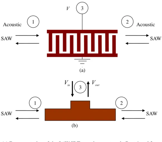
(19) Thus, the reference axis of transducer T3 gives. [W0 ] = [G1 ][ D2 ][W2 ] ,. (2.27). [W3 ] = [ D4 ][t5 ][ D6 ][G7 ][W7 ].. (2.28). and. By combining Eq. (2.25) through Eq. (2.28), the outward propagating SAW wave W7+ and W0− are related to the input a3 by ⎡W7+ ⎤ ⎡ 0 ⎤ = M [ ] ⎢ ⎥ + a3 [G1 ][ D2 ][τ 3 ] . ⎢W − ⎥ ⎣ 0 ⎦ ⎣ 0 ⎦. (2.29). In addition, a choice of matched conditions at input and output yields voltage values b3 = a7 = 0.. (2.30). At the output transducer T5 ,. [W5 ] = [ D6 ][G7 ][W7 ].. (2.31). Finally, the electrical output voltage Vout is derived from the scalar product Vout = b5 = [τ ] [W5 ] . T. 2.2. (2.32). Crossed-Field Model The crossed-field (Fig. 8) model is derived from Mason equivalent circuit model. employed for modeling acoustic bulk wave piezoelectric devices [18, 19, 21]. The equivalent circuits also have been widely used as approximate equivalent circuit for SAW IDTs [18, 22, 23]. In crossed-field model, the acoustic wave is represented by an electrical wave on a transmission line, and the piezoelectric energy conversion by a transformer. Moreover, the mechanical force and particle velocity at the acoustic ports are represented by its equivalent voltage and current, respectively. As a result, the equivalent circuits for SAW IDTs have two symmetric acoustic ports and one electric port, as shown in Fig. 9. In the terminology followed here, Port 1 and 2 represent electrical equivalent of “acoustic” ports, while Port 3 is. 10.

(20) a true electrical port.. 2.2.1 Electroacoustic Equivalences. All of three ports as shown in Fig. 9 are treated in equivalent electrical terms. At Port 1 and 2, the acoustic force F (in newtons) are transformed to electrical equivalent voltages V, while mechanical SAW velocities v are transformed to equivalent currents I. In terms of a common proportionality constant φ these transforms are V=. F. ,. (2.33). I = vϕ ,. (2.34). ϕ. where parameter φ is interpreted as the turns-ratio of an equivalent acoustic-to-electric transformer. This can be written in terms of electromechanical coupling coefficient K 2 , frequency f 0 , and total capacitance of the IDT, CT as. ϕ = 2 f 0CT K 2 Aρ v ,. (2.35). where ρ is the density of substrate and A is the effective crossed-sectional area.. 2.2.2 Admittance Matrix for IDT. Fig. 10 shows the unit cell of IDT and each model can be cascaded depending on number of pairs for sensor IDTs. Essentially, the IDTs are arranged acoustically in cascade and electrically in parallel. The equivalent current-voltage relations for a unit cell of IDT are given as ⎡ I1 ⎤ ⎡V1 ⎤ ⎢ I ⎥ = Y ⎢V ⎥ , ⎢ 2 ⎥ [ ]⎢ 2 ⎥ ⎣⎢ I 3 ⎦⎥ ⎣⎢V3 ⎦⎥. (2.36). where the 3×3 admittance matrix [Y] may be expanded as ⎡Y11 Y12 Y13 ⎤ [Y ] = ⎢⎢Y21 Y22 Y23 ⎥⎥ . ⎢⎣Y31 Y32 Y33 ⎥⎦. (2.37). 11.

(21) In order to calculate the overall response of the three acoustic transmission sub-matrices, ABCD matrix manipulations must be employed as shown in Fig. 11 [13]. ABCD matrix representation of a transmission line section of length d with equivalent electric impedance Z 0 on the unmetallized region, which is assumed to be a lossless transmission line segment, is ⎡ cos (θ ) Bu ⎤ ⎢ = 1 Du ⎥⎦ ⎢ j sin (θ ) ⎢⎣ Z 0. ⎡A [ Ru ] = ⎢Cu ⎣ u. jZ 0 sin (θ ) ⎤ ⎥. cos (θ ) ⎥ ⎥⎦. (2.38). The corresponding matrix [ Rm ] for a lossless metallized-strip may be represented by ⎡A [ Rm ] = ⎢Cm ⎣ m. ⎡ cos (θ m ) Bm ⎤ ⎢ = 1 sin (θ m ) Dm ⎥⎦ ⎢ j ⎢⎣ Z m. jZ m sin (θ m ) ⎤ ⎥. ⎥ cos (θ m ) ⎥⎦. (2.39). where the transit angle θ is obtained for the equivalent electric impedance Z 0 as. θ=. π f. .. 4 f0. (2.40). And, the transit angle θ m is obtained for the mechanical impedance Z m as. θm =. π f 2 fm. .. (2.41). From these, the total sub-matrix [ Rt ] for three cascaded sections of the transmission line in Fig. 10 is obtained as. [ Rt ] = [ Ru ][ Rm ][ Ru ].. (2.42). To obtain the total 2×2 ABCD matrix [Q] for the equivalent transmission line of the complete IDT with N t fingers, as shown in Fig. 12, the matrix in Eq.( 2.42) is cascaded to obtain ⎡Q. [Q ] = ⎢Q11 ⎣. 21. Q12 ⎤ N = [ Rt ] t . ⎥ Q22 ⎦. (2.42). Working backwards and employing ABCD-to-Y matrix conversions, the acoustic sub-matrix ⎡⎣Yaf ⎤⎦ for the total IDT is 12.

(22) ⎡Y f ⎡⎣Yaf ⎤⎦ = ⎢ 11f ⎣Y21. ⎡ Q22 Y12f ⎤ ⎢⎢ Q12 ⎥= Y22f ⎦ ⎢ 1 ⎢− Q ⎣ 12. −1 ⎤ Q12 ⎥ ⎥. Q11 ⎥ Q12 ⎥⎦. (2.43). Acoustic reflections from IDT fingers can lead to internal resonances and associated losses. Dealing with such losses required inclusion of an attenuation coefficient α f in a general ⎡⎣Y f ⎤⎦ -matrix representation for the IDT with finger reflections. In [13], the admittance matrix is approximated as ⎡ I1 ⎤ ⎡V1 ⎤ ⎢ I ⎥ ≈ ⎡Y f ⎤ ⎢V ⎥ , ⎢ 2⎥ ⎣ ⎦⎢ 2⎥ ⎢⎣ I 3 ⎥⎦ ⎢⎣V3 ⎥⎦. (2.44). where ⎡ Y11f Y12f ⎢ ⎡⎣Y f ⎤⎦ ≈ ⎢ Y21f Y22f ⎢ ⎢ −ϕ Gm tanh (α f + jθ m ) ϕ Gm tanh (α f + jθ m ) ⎣. −ϕ Gm tanh (α f + jθ m ). ⎤ ⎥ ⎥. ϕ Gm tanh (α f + jθ m ) ⎥ jωGT + 4 N tϕ 2Gm tanh (α f + jθ m ) ⎥⎦ (2.45). And 2×2 acoustic submatrix terms are given by Eq. (2.43). Solving Eq. (2.44) for the electrical admittance of the transducer, YL ( f ) , with the application of matched boundary conditions such that I1 = −V1 Z 0 = −V1G0 and I 2 = −V2 Z 0 = −V2G0 = I1 yields 2 (Y13 ) I YL ( f ) = 3 = . V3 ( G0 − Y11f − Y12f ) f. 2. (2.46). We consider the case shown in Fig. 13 where an acoustic wave is incident at Port 1, Port 2 is acoustically terminated, and Port 3 is electrically terminated in Z L ( f ) = 1 YL ( f ) . The transfer function with input and output voltage at port 3 can be obtained by simple electrical network analysis.. 2.3. Electromechanical Interaction The purpose of this section is to derive the electromechanical interaction due to a surface. electrode attached to the surface of a semi-infinite piezoelectric material [6, 33]. Let us 13.

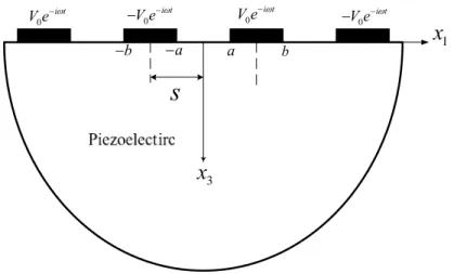
(23) consider the two-dimensional electroelastic problem concerned with the excitation of harmonic waves in a piezoelectric half-space, as shown in Fig. 14. The electrodes attached to the surface of the piezoelectric are assumed to be weightless, perfectly flexible and conducting, and have length W, which is assumed to be much larger than width. (λ 4). with. an important consequence that the electroelastic fields in the material are independent of the x2 -coordinate. The electroelastic fields in a piezoelectric are described by the following equation. The equations of move [24]: ∂σ 11 ∂σ 13 ∂ 2u + = ρ 21 , ∂x1 ∂x3 ∂t. (2.47). ∂σ 31 ∂σ 33 ∂ 2u + = ρ 23 . ∂x1 ∂x3 ∂t The equation of electrostatics: ∂D1 ∂D3 ∂φ ∂φ + = 0, E1 = − , E3 = − . ∂x1 ∂x3 ∂x1 ∂x3. (2.48). The equations of state:. σ 11 = C11E u1,1 + C13E u3,3 − e31φ,3 ,. σ 13 = C44E ( u1,3 + u3,1 ) − e15φ,1 , σ 33 = C13E u1,1 + C33E u3,3 − e33φ,3 ,. (2.49). D1 = e15 ( u1,3 + u3,1 ) − ε11S φ,1 , D3 = e31u1,1 + e33u3,3 − ε 33S φ,3 ,. where we denote, by σ ij , ui , Di , φi , ρ ,. ( i, j = 1,3) the. stress, the displacement, the. dielectric displacement, the potential, and the mass density, respectively. Accordingly, the problem reduces to the following system of (two-dimensional electroelastic) equations for the amplitude coefficients of the potential, φ , and displacement components, x1 and x3 C11E u1,11 + C44E u1,33 + ( C13E + C44E ) u3,13 − ( e31 + e15 ) φ,13 = ρ u&&1 ,. 14.

(24) (C. E 44. + C13E ) u1,13 + C44E u3,11 + C33E u3,33 − e15φ,11 − e33φ,33 = ρ u&&3 ,. (2.50). ( e15 + e31 ) u1,13 + e15u3,11 + e33u3,33 − ε11S φ,11 − ε 33S φ,33 = 0. Here and afterwards the harmonic time dependence e jωt is suppressed. Assume that the displacement and potential vectors are u = A ⋅ f (ξ ) ,. (2.51a). φ = φ0 ⋅ f (ξ ) ,. (2.51b). where ξ = k ⋅ x − ωt = ω ( s ⋅ x − t ) , and ω is angular frequency, k is wave vector, s is slowness vector in the x direction, and k =ω × s. Then ul , jk =. ∂ul = k j kk Al f ′′(ξ ), ∂x j ∂xk. d 2ui u&&i = 2 = ω 2 Ai f ′′(ξ ), dt. φ, jk. (2.52). ∂ 2φ = = k j kkφ0 f ′′(ξ ). ∂x j ∂xk. It follows that ⎡C11E s12 A1 + C44E s32 A1 + ( C13E + C44E ) s1s3 A3 − ( e31 + e15 ) s1s3φ0 − ρ A1 ⎤ f ′′ (ξ ) = 0, ⎣ ⎦ E E 2 E 2 2 2 ⎡ E ⎤ ′′ ⎣( C44 + C13 ) s1s3 A1 + C44 s1 A3 + C33 s3 A3 − e15 s1 φ0 − e33 s3 φ0 − ρ A3 ⎦ f (ξ ) = 0,. ⎡⎣( e15 + e31 ) s1s3 A1 + e15 s12 A3 + e33 s32 A3 − ε11S s12φ0 − ε 33S s32φ0 ⎤⎦ f ′′ (ξ ) = 0. If the second derivative of the disturbance f " (ξ ) exists, then we have an eigenvalue problem as follow: ⎡ A1 ⎤ M ⋅ ⎢⎢ A3 ⎥⎥ f ′′ (ξ ) = 0, ⎢⎣ φ0 ⎥⎦. (2.53). where. 15.

(25) ⎡C11E s12 + C44E s32 − ρ C13E + C44E ) s1s3 ( ⎢ C44E s12 + C33E s32 − ρ M = ⎢ ( C44E + C13E ) s1s3 ⎢ e15 s12 + e33 s32 ⎢ ( e15 + e31 ) s1s3 ⎣. − ( e31 + e15 ) s1s3 ⎤ ⎥ −e15 s12 − e33 s32 ⎥ , ⎥ −ε11S s12 − ε 33S s32 ⎥ ⎦. ⎛1 ⎞ s = ( s1 , s3 ) = ⎜ , η ⎟ . ⎝c ⎠. (2.54a). (2.54b). There exists a non-trivial solution if the determinant of Eq. (2.54a) vanishes, i.e., det ( M ) = 0 . Hence, three eigenvalues ηk2 must satisfy the bicubic equation of η 2 as. follows: Aη 6 + Bη 4 + Cη 2 + D = 0,. (2.55). where. (. ). A = −C44E C33E ε 33S − e332 , B=. 1 E 2 S (C44 c ρε 33 + C11E e332 + ρ c 2 e332 + e15 2C33E − C44E C33E ε11S − C11E C33E ε 33S 2 c + C13E 2ε 33S + 2e31e15C33E + e312C33E − 2C13E e13e33 − 2C13E e15e33 − 2C44E e31e33 + 2C13E C44E ε 33S ) 1 (− ρ c 2C33E ε11S − ρ c 2C44E ε11S − C44E c 2 ρε 33S − e312C44E + C11E C44E ε 33S 4 c + C11E C33E ε11S + 2 ρ c 2 e15e33 − 2C11E e15e33 − 2C13E C44E ε11S + 2C14E e31e15. C=−. + ρ 2 c 4ε 33S + e312 ρ c 2 + 2C13E e15 2 + ρ c 2 e15 2 − C13E 2ε11S − C11E ρ c 2ε 33S + 2e31e15 ρ c 2 ) D=−. 1 (−C11E ρ c 2ε11S + C11E C44E ε11S + ρ 2 c 4ε11S − C11E e15 2 − ρ c 2C44E ε11S + ρ c 2 e15 2 ) 6 c. The equation (2.55) can be directly solved by formula. It is noted that η k may be real or complex. For definiteness of single-value and bounded condition at infinity we assumed, Im (ηk ) ≥ 0.. (2.56). The corresponding four eigenvectors satisfy the proportional relation, k k A1( k ) A3( ) φ0( ) = = = Ck , p1k p2 k p3k. (2.57). where the superscript (k) denotes the k-th eigenvalue or eigenvector. The proportional factors. 16.

(26) pik are defined as p1k = s1η k ⎡⎣( C13E + C44E )( −e15 s12 − e33η k 2 ) + ( e31 + e15 ) ( C44E s12 + C33Eηk 2 − ρ ) ⎤⎦ , p2 k = ⎡⎣ − s12ηk 2 ( e31 + e15 ) ( C44E + C13E ) + ( e15 s12 + e33η k 2 )( C11E s12 + C44E η k 2 − ρ ) ⎤⎦ , p3k = ⎡( C11E s12 + C44E η k 2 − ρ )( C44E s12 + C332 η k 2 − ρ ) − s12ηk 2 ( C44E + C13E ) ⎢⎣. 2. ⎤. ⎥⎦. Hence, the displacement field may be assumed to be. u = P DC ei( k1x1 -ωt ) ,. (2.58). where. u =. {u1 u3 φ }. ⎡ p11 P = ⎢⎢ p21 ⎢⎣ p31. ⎡ eiωη1x3 ⎢ D=⎢ 0 ⎢ 0 ⎣. T. (2.59a) p13 ⎤ p23 ⎥⎥ p33 ⎥⎦. p12 p22 p32. 0 e. iωη2 x3. 0. (2.59b). 0 ⎤ ⎥ 0 ⎥, eiωη3 x3 ⎥⎦. (2.59c). ⎡ C1 ⎤ C= ⎢⎢C2 ⎥⎥ . ⎢⎣ C3 ⎥⎦. (2.59d). The unknown coefficients Ci must be determined by boundary conditions. It is a set of mechanical and electrical boundary conditions. The surface traction acting on an arbitrary horizontal plane is given by. σ 13 ( x1 , 0 ) = σ 33 ( x1 , 0 ) = 0.. (2.60). ( C1q11 + C2 q12 + C3q13 ) ei( k x −ωt ) = 0,. (2.61). ( C1q21 + C2 q22 + C3q23 ) ei( k x −ωt ) = 0,. (2.62). q1k = iC44E ( p1kη k + p2 k s1 ) − ie15 p3k s1 ,. (2.63). or 1 1. 1 1. where. 17.

(27) q2 k = iC13E p1k s1 + iC33E p2 kηk − ie33 p3kηk ,. k = 1, 2,3.. (2.64). The C1 , C2 , C3 satisfy the proportional relations, C3 C1 C2 = = = Q. q12 q23 − q13q22 q13q21 − q11q23 q11q22 − q12 q21. (2.65). Substitute these relations to Eq. (2.59) and the general form of displacement field is obtained. Then, u3 and φ0 have a general relation (proportional constant) with the first line of Eq. (2.59) divide by second.. 18.

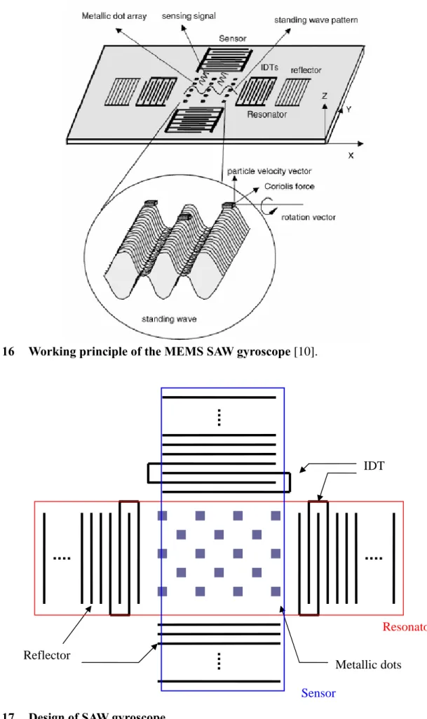
(28) Chapter 3 Design and Simulation of SAW Gyroscope. In this chapter, we present a preliminary design of SAW gyroscope using the COM theory, crossed-field model, and electromechanical interaction. The simulation work is done with MATLAB software package and the simulation results are listed together with the experimental data reported in the work of V. K. Varadan et al. [9] for comparison. For the design simplicity, we neglect the loss and attenuation of SAW propagation due to piezoelectric materials and metallic dots, bulk-wave conversion loss, and reflection and electrical interaction between metallic dots array, and etc.. 3.1. Surface Acoustic Wave Gyroscope. When a standing wave is generated on a piezoelectric material surface the anti-node v particles would vibrate in the vertical direction ( v in ± Z-direction). When substrate is v subjected to the angular rotation ( Ω in X-direction) perpendicular to the reference motion v v ( vv ) , the Coriolis force ( F = 2mΩ × vv in ± Y-direction) is produced in the direction perpendicular to the both vectors as shown in Fig. 15. Due to the wave motion along. X-direction, the Coriolis force acting on the surface particles along Y-direction would be distributed in the way of a wave motion. Base on the above-mentioned, the concept of utilizing SAW for the detection of rotation is described below and illustrated in Fig. 16. It consists of IDTs, reflectors, and a metallic dot array within the cavity, which are fabricated through micro fabrication techniques on the surface of a piezoelectric substrate. The metallic dots of mass m serve as proof mass for this gyroscope. The resonator IDTs create SAW that propagates back and forth between the reflectors and forms a standing wave pattern within the cavity due to the collective reflection from reflectors. SAW reflection from individual metal strips adds in phase if the reflector periodicity is equal to half a wavelength. For the established standing wave pattern in the cavity as explained in Fig. 16, a typical substrate particle at the nodes of standing wave has no amplitude of deformation in the Z-direction. However, at or near the anti-nodes of standing wave pattern, such particles experience larger amplitude of vibration in the Z-direction, which 19.

(29) serves as the reference vibrating motion for this gyroscope. Metallic dots of mass (m), which serve as the proof mass, are placed in the resonator region where standing waves are formed. To amplify the magnitude of the generated Coriolis force in phase, the metallic dots are v positioned strategically at the anti-node locations. The rotation ( Ω in X-direction)) v perpendicular to the velocity ( v in ± Z-direction) of the oscillating masses (m) produces v v v Coriolis force ( F = 2mΩ × v in ± Y-direction) in the direction perpendicular to the both vectors as shown in Fig.16. Since this Coriolis force is applied on a piezoelectric substrate, it generates a secondary SAW in the Y-direction with same frequency as the reference oscillation. The metallic dot array is placed along the Y-direction such that the SAW due to the Coriolis forces adds up coherently. The generated SAW is received by the sensing IDTs placed in the Y -direction [10]. The design of SAW gyroscope is subdivided to two parts, SAW resonator and sensor, as shown in Fig. 17. The former is to generate reference vibrating motion for proof mass; the latter can detect the Coriolis force with voltage output due to rotation from proof mass. It is important to know the characteristics of impedance, admittance, bandwidth and sensitivity near the operating frequency of the SAW gyroscope, because the sensing IDTs have to be designed such that they efficiently pick the SAW wave generated due to Coriolis force. The numerical simulation of the SAW resonator is done by coupling-of-modes (COM) theory because a SAW devices can be easily represented by several basic elements as discussed in Chap. 2. The SAW sensor is modeled using crossed-field model instead of COM theory due to the input to “SAW sensor” is the Coriolis force, not a voltage signal. Furthermore, to estimate the Coriolis force, we need to know the particle vibrating velocity in advance. Therefore, the “electromechanical interaction” method discussed in Chap. 2 is utilized to convert the transmitted power into exact particle displacement, so as to obtain the velocity term in the Coriolis force.. 3.2. Preliminary Design of SAW Gyroscope. 3.2.1. Operating Frequency. The periodicity of IDTs and reflectors, and the separation between the reflector gratings determine the operation frequency of the device. This device can be operating at higher 20.

(30) frequency with smaller device size or lower frequency with a larger device size. Generally, the frequency range of SAW filters is about 10M ~ 3G Hz. The SAW gyroscope which is similar to SAW filters might also be working at the range of GHz. However, for the comparison purpose, we design the operation frequency of our SAW gyroscope in accordance with data shown in [9] and [10]. In that regard, the SAW gyroscope has the minimum feature of about 6 µm and 75 MHz for the operation frequency. 3.2.2. Substrate In view of the working principle discussed above, any piezoelectric material such as. lithium niobate, lithium tantalite, or quartz can be used as a substrate. For efficient generation and detection of SAWs through IDTs, 128o YX LiNbO3 is chosen as a piezoelectric substrate due to its rather high electromechanical coupling. The material properties of 128o YX LiNbO3 are shown in Appendix. A few things to be noted that: Firstly, this electromechanical coupling coefficient ( K 2 ) in X-direction is different from that in. Y-direction, which is determined by formula [25]. Secondly, the wave velocity is different in the X- and Y-directions due to the anisotropy of 128o YX LiNbO3 , which measured as 3961 m s and 3656 m s , respectively. The errors between published data (3992 m s , as shown in Appendix) and the experimental results are mainly due to the effect of metallization and the metallic dot array [9], which will be discussed later. 3.2.3. Interdigital Transducer. The design of Interdigital transducer (IDT) of SAW gyroscope is similar to IDT existed in other SAW devices, and they are in charge of exciting and sensing the propagation wave. The IDTs are electrodes patterned on the piezoelectric substrate and a periodic strain field is generated in the piezoelectric crystal that produces propagating surface acoustic wave, when an alternating voltage is applied. This propagation wave gives rise to a standing wave when the propagating waves are launched in both directions away from the transducer. The transducer electrodes may be either gold or aluminum. The design of interdigital transducers of both of resonator and sensor is shown in Fig. 18, which utilized aluminum as the material of electrodes. According to [9], to obtain good resonator performance with this high-coupling-coefficient substrate, the constant finger 21.

(31) overlap or aperture of IDTs should be minimized, but it needs to be large enough to avoid acoustic beam diffraction. The aperture (W) of IDTs at two ends should be large enough so that the metal dots array is located within the apertures of IDTs. Fig. 19 shows the simulation result of the numbers of IDT electrodes vs. transmitted power, while keeping the reflector design the same in a resonator. The calculation in the simulation is based on the COM theory. As shown in plot, the maximum power transmitted took place at the 11 electrodes and 45 electrodes respectively. Here we choose 11 electrodes for the IDT resonator design to minimize the size of SAW gyroscope. On the other hand, Fig. 20 shows the IDT output voltage vs. number of electrodes, while keeping the input force the same. The calculation in the simulation is based on the crossed-field model. As it shows in the plot, the maximum output voltage takes place at 89 electrodes. Therefore we choose 89 electrodes for sensor IDT design.. 3.2.4. Reflector. SAW reflection from individual metal strips adds in phase if the reflector periodicity is equal to half a wavelength Λ = λ0 2 [10]. The transmitted power with different fingers of reflector of SAW resonator on two ends is shown in Fig. 21. The curve has periodicity and its period is about 45. From this figure, higher reflectivity with larger fingers of reflector is not revealed and the reasons for it are not clear to us at this point. In spite of this, we choose 47 fingers for reflector for minimize the size of device.. 3.2.5. Spacing. The separation between each component is chosen as an integral number of half wavelengths so that the standing waves can be created within the cavity.. 3.2.6. Metallic Dot Array. Metallic dots are placed within cavity in between IDTs on two ends. They fluctuate up-and-down along with the surface wave motion, and serves as the proof mass for the generation of Coriolis force. The material of metallic dot is chosen to be gold due to its large density (ρ) can provide large mass at small size. Their shapes were rectangles (almost squares) and each side was equaled to quarter of wavelength of both direction (X- and Y-direction) 22.

(32) respectively. The dimensions of the dot arrays are designed slightly smaller than aperture (W) of their corresponding IDTs to minimize the effects of wave front distortion at the edges of the IDT electrodes. There are 15 ×15 of metallic dots in this design case.. 3.3. Transformation of Coriolis force. So far, the design for the IDT resonator is done by the COM theory and the IDT sensor is done by the crossed-field model. The output of the COM theory is the square root of power of transmitted wave, while the input of the crossed-field model is the input force from Coriolis force. Therefore, we need to find a way to obtain the particle velocity out of the transmitted power so as to calculate the Coriolis force. In the COM theory, when input ports are a3 and a5 ( a3 = a5 ), and b3 = b5 = 0 (see Fig. 7), [W3 ] or [W4 ] is the output of resonator and will be the reference vibration motion of particle velocity for the calculation of Coriolis force. This Coriolis force is then the input of sensor IDT when it subjected to rotation. The mean power carried by a Rayleigh wave beam of width W is given in terms of surface electric potential by [17]: 1 2 P = α2 Φ , 2. 1. ⎛ ωWC0 ⎞ 2 α =⎜ ⎟ , 2 ⎝ K ⎠. (3.1). where α is a potential/power conversion factor with units ⎡⎣W 1 2 V ⎤⎦ and derives from piezoelectric permittivity method. In COM theory, 28, 29] and then, the wave amplitude is. [Wi ]. [Wi ] = α Φ .. 2. is the transported power [26, 27,. There exists a relation among the. surface electrical potential and particle displacement as we mentioned in section 2.3. Therefore, the particle displacement can be estimated. As shown in Eq. (2.65), we need to find out the Q, which is defined as the rate of energy transferred across a unit area, to proceed on the power-displacement conversion. Here, we introduce the Poynting vector [30], defined by. Pj ( x j , t ) = −σ ij. ∂D j ∂ui +φ . ∂t ∂t. (3.2). 23.

(33) Here the first term on the right hand side is the acoustic part of the Poynting vector and the second represents the electrical contribution. Its dimension is the power per unit area. The detail information of Poynting vector can be found in [30] and it says that, if there is an internal source in a volume V, the radiated power is P = ∫ P ⋅ n dS .. (3.3). S. S is the surface in volume and n is a unit vector normal to the surface. We assume that the amplitude of. [Wi ]. 2. which deduced from COM theory is the radiated power. Thus, the. constant Q can be found approximately and then u3 in Eq. (2.59a). In [10], it shows that 128o YX Lithium niobate has 2 Å Z-displacement per a unit surface potential and these experimental results agree with our numerical simulations. The Coriolis force could be calculated by F = 2mΩv3 , where v3 = u&3 = iωu3 for the mass dots. This Coriolis force is then fed into the crossed-field model to calculate for the IDT output voltage.. 3.4. Estimation of Sensing Resolution for SAW Gyroscopes The sensing resolution of the proposed SAW gyroscopes with 90 and 89 fingers of. sensor IDT are shown in Fig. 22 and Fig.23, respectively. The 89 electrodes design of the sensing IDT is the optimal design for the voltage output according to our simulations. The experimental data reported in Varadan et al. [9, 10], in which 60 electrodes were used, is shown in the same plot for comparison. As shown in the plot, the sensing resolution predicted by our approach (89 electrodes) is different from the experimental data, while the 90 electrodes design is close to the experimental data.. 3.5. Discussion As shown in Fig. 19 and Fig. 20, the transmitted power does not increase along with the. number of IDT electrodes; neither the voltage output of the IDT sensor increase along with the number of IDT electrodes. Besides, Fig. 21 also didn’t show the higher reflectivity with larger fingers of reflector. These simulation results somehow contradict with our intuition of IDT functionality. These simulation results will be investigated in future.. 24.

(34) The deviation of our prediction and experimental data, as shown in Fig. 22 and Fig. 23, may come from the way we combined the COM theory and crossed-field model to model the whole system. For example, the input to crossed-field model should be both of particle force and velocity. However, in this simulation, we used Coriolis force as the force input while the velocity is obtained by assuming the maximum power transmission. This could be erroneous and should be investigated later on. Furthermore, we have assumed that the metallic dot arrays have no effect on the transmitted power generated by the IDT resonator, but to generate Coriolis force the sensing IDT. The assumption is obviously impractical since the metallic dots have mass loading on the surface wave motion. Besides, the edges of metallic dots could cause diffraction and interfered with the wave propagation along Y-direction. All these effect will need further investigation.. 25.

(35) Chapter 4 Conclusion and Future Work. 4.1. Conclusion In this work, the design of a gyroscope, consisted of surface acoustic wave (SAW). resonator and sensor, is presented. The SAW resonator is designed and optimized using COM theory, while the design of SAW sensor is based on the crossed-field model. The output of the COM theory is the square root of power of transmitted wave in SAW resonator, while the input to the SAW sensor needs to be the force for crossed-field modeling. We have successfully used the “electromechanical interaction” method to obtain a relation between surface potential and particle displacement, so as to obtain the particle velocity for the calculation of Coriolis force. The simulation results shows that the optimal performance can be achieved by 11 electrodes of the IDT, 47 electrodes of the reflector in the SAW resonator at both ends; 89 electrodes of the IDT in the SAW sensor. This design is different from what shown in the report [9, 10]. The deviation could be due to the way we combined COM theory and crossed-field model, and the mass loading from metallic dots.. 4.2. Future Works The more complete simulations and experiments must be done in the future. Some. future works are listed below. 1.. Better understand the methods utilized for the SAW devices analysis.. 2.. Analyze the behavior of the metallic dot array in the cavity between IDTs in two ends.. 3.. Implement the SAW gyroscope when the analyses work is completed.. Other than that, the effects of metallic dot array contain mass loading, reflection, and electrical interaction. Further investigation will be needed to take all these effect into consideration. One possible approach to model the mass loading effect from metallic dots could be treating them as a reflector in a SAW device since they are located in a way similar 26.

(36) to parallel strips in view of the one-dimension propagation waves. If so, they can be simulated by various methods such as piezoelectric permittivity method, impulse response model, COM theory, and etc.. 27.

(37) Reference [1]. N. Yazdi, F. Ayazi, K. Najafi, “Micromachined Inertial Sensors,” Proceedings of the IEEE, Vol.86, No.8, pp.1640-1659, Aug. 1998.. [2]. S. Park, “Adaptive Control Strategies for MEMS Gyroscopes," University of California, Berkeley, Department of Mechanical Engineering, Ph.D. Thesis, 2000.. [3]. D. S. Ballantine, Acoustic wave sensors: theory, design, and physico-chemical applications, Academic Press, Boston, 1996.. [4]. D. S. Ballantine et al. “Acoustic wave sensors /theory, design, and physico-chemical application,” Academic Press, Boston, 1996.. [5]. 吕志清, 胡爱民, “MEMS-IDT声表面波陀螺,” Micronanoelectronic Technology, Vol.40, No.4, 2003.. [6]. FuQian Yang, “Electromechanical Interaction of Linear Piezoelectric Materials with a Surface Electrode,” Journal of Materials Science, Vol.39, No.8, pp.2811-2820, 2004.. [7]. B. Y. Lao, “Gyroscopic effect in surface acoustic waves,” IEEE Transactions on Sonic and Ultrasonic, Vol.28, No.5, pp.687-691, 1980.. [8]. M. Kurosawa, Y. Fukuda, M. Takasaki, T. Higuchi, “A surface-acoustic wave gyro sensor,” Sensors and Actuators A-Physical, Vol.66, No.1-3, pp.33-39, Apr. 1998.. [9]. V. K. Varadan, W. D. Suh, P. B. Xavier, K. A. Jose, V. V. Varadan, “Design and development of a MEMS-IDT gyroscope,” Smart Materials & structures, Vol.9 No.6, pp.898–905, Dec. 2000.. [10]. K. A. Jose, W. D. Suh, P. B. Xavier, V. K. Varadan, V. V. Varadan, “Surface acoustic wave MEMS gyroscope,” Wave Motion, Vol.36, No.4, pp.367-381, Oct. 2002.. [11]. V. K. Varadan, K. A. Jose, P. Xavier, D. Suh, V. V. Varadan, “Conformal MEMS-IDT gyroscopes and their performance comparison with fiber optic gyroscope,” in: V.K. Varadan (Ed.), Proceedings of the SPIE Symposium on Smart Electronics and MEMS, Vol.3990, pp. 335–344, 2000.. [12]. R. C. Woods, H. Kalami, B. Johnson, “Evaluation of a Novel Surface Acoustic Wave Gyroscope,” IEEE Transactions on Ultrasonics, Ferroelectrics, and Frequency Control, Vol.49, No.1, pp.136-141, Jan. 2002.. [13]. C. K. Campbell, Surface Acoustic Wave Devices for Mobile and Wireless Communications, Academic Press, New York, 1998.. [14]. J. R. Pierce, “Coupling-of-modes of propagation,” Journal of Applied Physics, Vol.25, No.2, pp.179-183, Feb. 1954.. [15]. P. S. Coss, R. V. Schmidt, “Coupled surface acoustic wave resonator,” Bell System Technical, Journal, Vol.56 No.8, pp.1447-1481, Oct. 1977.. [16]. H. Haus, P. V. Wright, “The Analysis of Grating Structures by Coupling-of-Modes Theory,” Proceedings of the IEEE Ultrasonics Symposium, Vol.1 pp. 277-281, Nov. 1980.. 28.

(38) [17]. D. Royer, E. Dieulesaint, Elastic waves in Solids Ⅱ: Generation, Acousto-optic Interaction, Applications, Springer-Verlag, Berlin, 2000.. [18]. W. R. Smith, H. M. Gerard, J. H. Collins, T. W. Reeder, H. J. Shaw, “Analysis of Interdigital Surface Wave Transducers by Use of an Equivalent Circuit Model,” IEEE Transactions on Microwave Theory and Techniques, Vol.17, No.11, pp.856-864, Nov. 1969.. [19]. W. R. Smith, Jr., “Studies of Microwave Acoustic Transducers and Dispersive Delay Lines,” Stanford University, Department of Applied Physics, Ph.D. Thesis, pp.1-147, 1969.. [20]. W. P. Mason, “Electromechanical Transducers and Wave Filters,” van Nostrand-Reinhold, 2nd Edition, Princeton, New Jersey, pp.201-209, pp.399-409, 1948.. [21]. W. R. Smith, H.M. Gerard, J. H. Collins, T. W. Reeder, H. J. Shaw, “Design of surface wave delay lines with interdigital transducers,” IEEE Transactions on Microwave Theory and Techniques, Vol.17, No.11, pp.865-873, Nov. 1969.. [22]. W. R. Smith, “Experimental Distinction Between Crossed-Field and In-Line Three-Port Circuit Models for Interdigital Transducers,” IEEE Transactions on Microwave Theory and Techniques, Vol.22, pp.960-964.. [23]. W. R. Smith, H.M. Gerard, W. R. Jones, “Analysis and Design of Dispersive Interdigital Surface-Wave Transducers,” IEEE Transactions on Microwave Theory and Techniques, Vol.20, No.7, pp.458-471, 1972.. [24]. V. Parton, B. Kudryavtsev, N. Senik, J. Tani, “Rayleigh Waves Excitation Using a Pair of Oppositely Charged Electrodes,” International Journal of Applied Electromagnetics in Materials, Vol.5, No.4, pp.291-310, 1994.. [25]. 周卓明，壓電力學，全華，台北，2003。. [26]. S.V. Biryukov, G. Martin, V. G. Polevoi, M. Weihnacht, “Derivation of COM Equations Using the Surface Impedance Method,” IEEE Transactions on Ultrasonics, Ferroelectrics, and Frequency Control, Vol.42, No.4, pp.602 – 611, 1995.. [27]. K. Nakamura, “A Simple Equivalent Circuit for Interdigital Transducers Based on the Coupled-Mode Approach,” IEEE Transactions on Ultrasonics, Ferroelectrics, and Frequency Control, Vol.40, No.6, pp.763 -767, 1993.. [28]. Dong-Pei Chen, A. H. Herman, “Analysis of Metal-Strip SAW Gratings and Transducers,” IEEE Transactions on Sonic and Ultrasonic, Vol.SU-32, No.3, pp.395-408, 1985.. [29]. W. Soluch, “Admittance Matrix of a Surface Acoustic Wave Interdigital Transducer,” IEEE Transactions on Ultrasonics, Ferroelectrics, and Frequency Control, Vol.40, No.6, pp.828-831, 1993.. [30]. D. Royer, E. Dieulesaint, Elastic Waves in Solids Ⅰ: Free and Guided Propagation, Springer-Verlag, Berlin, 2000.. [31]. Y. C. Fung, Foundations of Solid Mechanics, Prentice-Hall, 1965.. [32]. J. W. Gardner, V. K. Varadan, O. O. Awadelkarim, Mircosensors MEMS and Smart Devices, John Wiley & Sons, 2001. 29.

(39) [33]. W. Matthijs den Otter, “Approximate Expressions for the Capacitance and Electrostatic Potential of Interdigital Electrodes,” Sensors and Actuators A, Vol.96, No.2-3, pp.140-144, 2002.. 30.

(40) LIST OF FIGURES. Ω a = 2Ω × v. Fig. 1. The Coriolis effect [1].. 31.

(41) Fig.2a. Displacement of particles on the surface of half space due to the Rayleigh wave [31].. Fig. 2b Interdigital transducer, formed by patterning electrodes on the surface of a piezoelectric crystal, for exciting surface acoustic wave: (a) SAW electrical potential, (b) plan view, (c) side view [4].. 32.

(42) Sensor IDT. Generator IDT. Perturbation Masses Reflector. Fig. 3. Configuration of the IDTs, the reflectors and the perturbation electrodes.. Fig. 4. (a) Basic elements of gyroscope: IDT, acoustic spacing and reflector. (b) Schematic representation of a SAW devices using transmission matrix [9].. 33.

(43) Λ Wi −+1. Wi +. Wi −−1. Wi −. ith element of SAW reflection grating of length L. Fig. 5. The SAW reference planes at the ith element of a SAW reflection grating of length L [13].. Electrical. a. SAW. 3. b. Reference plane. Wi −+1. Wi +. Wi −−1. Wi −. 1 Acoustic. Fig. 6. SAW. 2. Λ. Λ. 4. Acoustic. 4. Schematic representation of electrical and acoustic ports [13].. 34.

(44) Fig. 7. Schematic matrix representation of a two-port SAW resonator [9].. L =Half-wavelength −. −. +. E. E. Fig. 8. An instantaneous E-field direction in the crossed-field model [32].. 35.

(45) V. 3. 1. Acoustic. 2. Acoustic. SAW. SAW. (a). Vin. 3. Vout. 1. 2. SAW. SAW (b). Fig. 9. (a) Representation of the SAW IDT as a three network, Port 1 and 2 are normally assigned to the “ acoustic” ports, while Port 3 is the electrical port. (b) In the crossed-field model, acoustic signals at Port 1 and 2 are converted to equivalent electrical transmission-line parameters [13].. I1. jZ 0 tan (θ 2 ). − jZ 0 csc (θ ). jZ 0 tan (θ 2 ). jZ m tan (θ m 2 ). jZ m tan (θ m 2 ). jZ 0 tan (θ 2 ). V1 ϕ :1. V2. 2. ϕ :1. I3 V3. Fig. 10. I2. − jZ 0 csc (θ ). − jZ m csc (θ m ). Cs. ϕ :1. jZ 0 tan (θ 2 ). Crossed-field model of equivalent circuit representation [13].. 36.

(46) ⎡ cosh ( kd ) Z 0 sinh ( kd ) ⎤ ⎡A B⎤ ⎢ ⎥ ⎢C D ⎥ = ⎢ 1 sinh ( kd ) cosh ( kd ) ⎥ ⎣ ⎦ ⎢Z ⎥⎦ ⎣ 0. ⎡ A1 ⎢C ⎣ 1. B1 ⎤ D1 ⎥⎦. ⎡V1 ⎤ ⎡ A1 ⎢ I ⎥ = ⎢C ⎣ 1⎦ ⎣ 1. ⎡ A2 ⎢C ⎣ 2. B2 ⎤ D2 ⎥⎦. ⎡ An ⎢C ⎣ n. B2 ⎤ ⎡ An L D2 ⎥⎦ ⎢⎣Cn. B1 ⎤ ⎡ A2 D1 ⎥⎦ ⎢⎣C2. Bn ⎤ Dn ⎥⎦. Bn ⎤ ⎡Vn ⎤ Dn ⎥⎦ ⎢⎣ I n ⎥⎦. Fig. 11 (a) The ABCD matrix representation of a transmission-line section of length d, with characteristic impedance Z 0 and propagation constant k. (b) The matrix evaluation of cascaded two-port networks [13].. 37.

(47) I1 V1. i0. ν0 i 31. 1. i1. 1. i2. 2. ν1. ν 31. i32. ν 32. I3. V3. ν2. iNt −1. iN t. ν N −1. Nt. i3 Nt. ν 3N. t. I2. νN. t. t. V2 2. 3. Fig. 12 Transducer composed N t number of fingers, acoustically in cascade and electrically in parallel [18].. I1. I2. V1. V2. I3. V3. Fig. 13 Block diagram of receiving transducer configurations. Transducer with acoustic generator at port 1.. 38.

(48) V0 e − iωt. V0 e − iωt. −V0 e− iωt. −a. −b. a. −V0 e− iωt b. x1. s x3. Fig. 14 Layout of the system for the excitation of surface Rayleigh waves in a piezoelectric medium.. Z Y X. Fig. 15. Coriolis forces acting on particles [8].. 39.

(49) Fig. 16. Working principle of the MEMS SAW gyroscope [10].. IDT. Resonator Reflector. Metallic dots Sensor. Fig. 17. Design of SAW gyroscope. 40.

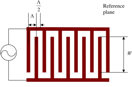
(50) Λ. Λ 2. Reference plane. W. Fig. 18. The design of interdigital transducer.. Fig. 19. Result of the numbers of RIDT electrodes vs. transmitted power.. 41.

(51) Fig. 20. SIDT output voltage vs. number of electrodes of SIDT.. Fig. 21 The transmitted power with different fingers of reflector of SAW resonator on two ends. 42.

(52) Fig. 22 The sensing resolution of the proposed SAW gyroscopes with 90 fingers of sensor IDT and calculated data by Varadan et al. [10]. Fig. 23 The sensing resolution of the proposed SAW gyroscopes with 89 fingers of sensor IDT and calculated data by Varadan et al. [10]. 43.

(53) Appendix Material constants for LiNbO 3 z. Density:. 4700 kg. z. Symmetry class:. Triangle 3m. m3. z. Compliance ⎡ S11 S12 S13 ⎢S ⎢ 12 S11 S13 ⎢ S13 S13 S33 S IJ = ⎢ ⎢ S14 − S14 0 ⎢0 0 0 ⎢ 0 0 ⎣⎢ 0. S14. 0. − S14. 0. 0. 0. S44. 0. 0. S 44. 0. 2S14. (. Compliance Constants 10−12. ⎤ ⎥ 0 ⎥ ⎥ 0 ⎥ 0 ⎥ ⎥ 2S14 ⎥ 2 ( S11 − S12 ) ⎦⎥ 0. m 2 newton. ). S IJ. S11 S33 S 44 S12 S13 S14 5.78 5.02 17.0 -1.01 -1.47 -1.02. z. Stiffence 0 0 ⎡ C11 C12 C13 C14 ⎤ ⎢C ⎥ 0 ⎢ 12 C11 C13 −C14 0 ⎥ ⎢C13 C13 C33 ⎥ 0 0 0 ⎢ ⎥ CIJ = C14 −C14 0 C44 0 0 ⎢ ⎥ ⎢ 0 ⎥ 0 0 0 C44 C14 ⎢ ⎥ 1 ⎢ 0 0 0 0 C14 ( C11 − C12 )⎥⎥ ⎢⎣ 2 ⎦ 10 2 newton m CIJ Stiffence Constants 10. (. ). C11 C33 C44 C12 C13 20.3 24.5 6.0 5.3 7.5 z Piezoelectric Strain 0 0 0 d15 −2d 22 ⎤ ⎡ 0 ⎢ diJ = d Ji = ⎢ − d 22 d 22 0 d15 0 0 ⎥⎥ ⎢⎣ d31 d31 d33 0 0 0 ⎥⎦. (. Piezoelectric Strain Constants 10−12 d15 68. d 22 21. coulomb newton d31 -1. 44. C14 0.9. d33 6. ). diJ = d Ji.

(54) z. Piezoelectric Stress 0 0 ⎡ 0 ⎢ eiJ = eJi = ⎢ −e22 e22 0 ⎢⎣ e31 e31 e33. e15 0. Piezoelectric Stress Constants. −2e22 ⎤ 0 0 ⎥⎥ 0 0 ⎥⎦ coulomb m 2 e15. 0. (. ). eiJ = eJi. e15 e22 e31 e33 3.7 2.5 0.2 1.3. z. Relative Permittivity ⎡ε11S 0 0⎤ ⎢ ⎥ T S ⎣⎡ε ij ⎦⎤ = ⎣⎡ε ij ⎦⎤ = ⎢ 0 ε11 0 ⎥ ⎢ 0 0 ε 33S ⎥ ⎣ ⎦. ⎡ε11T 0 0⎤ ⎢ ⎥ T = ⎢ 0 ε11 0 ⎥ T ⎥ ⎢ 0 0 ε 33 ⎣ ⎦ Relative Permittivity Constants for Piezoelectric Materials. ε11S ε 0. ε 22S ε 0. ε 33S ε 0. ε11T ε 0. T ε 22 ε0. ε 33T ε 0. 44. -. 29. 84. -. 30. ε 0 = 8.854 ×10. −12. fards m. 45.

(55)