西太平洋大陸棚區衛星測高應用之改善(III)

(1)

行政院國家科學委員會專題研究計畫成果報告

西太平洋大陸棚區衛星測高應用之改善(3/3)

計畫類別：個別型計畫計畫編號： NSC93-2611-M-009-001- 執行期間： 93 年 08 月 01 日至 94 年 07 月 31 日執行單位：國立交通大學土木工程學系(所) 計畫主持人：黃金維計畫參與人員：徐欣瑩，劉祐廷，董曉鈞，郭金運報告類型：完整報告處理方式：本計畫可公開查詢

中華民國 94 年 11 月 1 日

(2)

行政院國家科學委員會補助專題研究計畫■成果報告

西太平洋大陸棚區衛星測高應用之改善（

3/3）

計畫類別：■ 個別型計畫 □ 整合型計畫

計畫編號：

NSC

NSC 93-2611-M-009-001

執行期間： 93 年 8 月1日至 94 年 7 月 31日

計畫主持人：黃金維

計畫參與人員：徐欣瑩，劉祐廷，董曉鈞，郭金運

成果報告類型(依經費核定清單規定繳交)： ■完整報告

(3)

Summary of the three-year project

This is a three-year project aiming to improve coastal applications of satellite altimetry. After a three-year work, most of the objectives of this project have been achieved. In the previous reports, shallow-water tide models over western Pacific have been established and published. This current report summarizes the work for 8/1/2004-7/31/2005 and consists of two parts:

Part I: presents improved methods to compute shallow-water gravity anomalies. The paper associated with Part I has been submitted to Journal of Geodynamics (SCI journal) for review in May 2005.

Part II: shows the techniques of waveform retracking as a mean to improve altimeter data quality over shallow water and how retracked Geosat/GM data are used gravity computation. The paper associated with Part II has been submitted to Journal of Geodesy (SCI journal) for review in September 2005.

(4)

PART I: Gravity anomaly from satellite altimetry over shallow waters:

case studies in the East China Sea and Taiwan Strait

Gravity anomaly from satellite altimetry over shallow waters: case

studies in the East China Sea and Taiwan Strait

1. Introduction

Satellite altimetry over shallow waters has been very useful in geodetic, geophysical and oceanographic applications. Recent compilations of such altimetric applications are, e.g., Fu and Cazenave (2001) and Hwang et al. (2004). One example of geodetic application is coastal gravity field modeling: use of combined coastal altimetry data with terrestrial gravity anomalies has resulted in gravity field models that outperform models using only terrestrial gravity data (Li and Sideris, 1997; Andersen and Knudsen, 2000). Furthermore, the potential of satellite altimetry in determining sea surface topography has also been exploited in Hipkin (2000). Sea surface topography is the essential parameter for a world vertical datum (Rapp and Balasubramania, 1992). For oceanographic applications, shallow-water altimetry has been used to derive M-2 internal tides (Niwa and Hibiya, 2004) and variations of surface circulations (Yanagi et al., 1997). Examples of geophysical applications of altimetry are abundant in the literature; we refer to Cazenave and Royer (2001) for a comprehensive review.

Altimeter-gravity conversion is one of the most important aspects of the geodetic and geophysical applications of satellite altimetry. Currently, the achieved accuracies of altimeter-derived gravity anomalies vary from one oceanic region to another, depending on gravity roughness, altimeter data quality and density; see also the accuracy assessments in Sandwell and Smith (1997), Hwang et al. (2002) and Andersen et al. (2005). The accuracy analyses associated with these global gravity anomaly grids are mostly over the open oceans. As pointed out by Hwang and Hsu (2004), altimeter data over shallow waters are prone to errors in altimeter radar ranges and errors in geophysical corrections. When using inferior or erroneous altimeter data, the resulting gravity anomalies may contain artifacts that lead to a false interpretation of the underlying phenomenon.

The East China Sea (SCS) and the Taiwan Strait (TS) are two typical shallow-water areas. Here the gravity fields are relatively smooth, but gravity lows and highs occur over regions with thick sediments and at the margin of the continental shelf. Fig. 1 shows the depths and the distribution of shipborne gravity data in the ECS and the TS. In the ECS, one publicly accessible database of shipborne gravity data is with the National Geophysical Data Center (NGDC) (http://www.ngdc.noaa.gov), and the data

(5)

are quite sparsely distributed. In the TS, the shipborne gravity data were mostly collected by research vessels studying marine plate tectonics around Taiwan. A recent data set of shipborne gravity was compiled by Hsu et al. (1998). Global altimeter-derived gravity anomaly grids have been important sources of gravity anomalies in these areas. Due to the shallow-water nature of these areas, the procedures used in the derivations of global grids may not be optimal. Therefore, it is expected the accuracy of altimeter-derived gravity anomalies can be improved. Also, it is possible to further improve the gravity accuracy by using a different altimeter data type than commonly used ones such as sea surface height (SSH) and deflection of the vertical (DOV). With these problems as the background, the objective of this paper is therefore to investigate many issues of altimeter-gravity conversion over shallow waters, and to carry out case studies over the ECS and the TS.

2. Comparison of three global gravity grids over ECS and TS

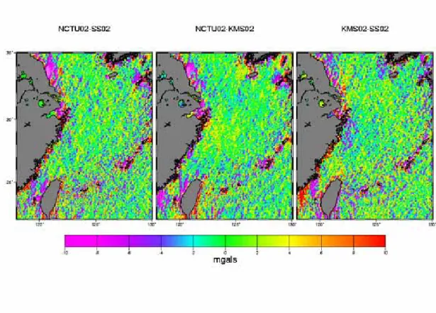
Our investigation begins with a comparison among three global, altimeter-derived gravity anomaly grids over the ECS and the TS. The three grids were computed by Sandwell and Smith (1997), Andersen et al. (2005), and Hwang et al. (2002). They are designated as SS02, KMS02 and NCTU02, respectively. Table 1 shows statistics of differences over areas of various depths. Table 1 shows no clear correlation between depth and gravity anomaly difference. This can be explained as follows: since these authors used similar altimeter data sets in the gravity computations, some of the systematic errors due to bad altimeter data are eliminated when differencing any two grids. Fig. 2 shows the distributions of the three sets of gravity anomaly differences. As expected, for all the three sets, large differences occur over the waters off the coasts of China, Japan, Korea, and the Ryukyu Island Arc. A major portion of the TS contains large differences. It is noted that, areas distant from the coasts might also contain large differences, e.g., a spot off the east coast of China centering at about latitude= 28°N and longitude = 124°E.

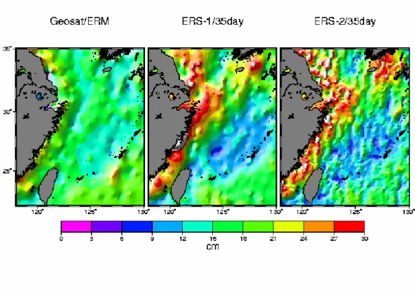
In order to see the possible causes of the differences in the three grids, we investigate the qualities of SSHs and current tide models over these two regions.Fig. 3 shows the standard errors of the mean SSHs from the Geosat/ERM, ERS-1/ 35 day and ERS-2/35 day repeat missions. The standard errors of Geosat/ERM SSHs are relatively small because a large number of repeat cycles (68 cycles) were used, compared to only 26 cycles used in averaging ERS-1 and ERS-2 repeat SSHs. The patterns of error distributions of ERS-1 and ERS-2 are similar: large standard errors occur in the coastal areas of China, Taiwan, Korea and Japan. As the depth decreases, the standard error of SSH increases. Comparing Figs. 2 and 3, it is clear that gravity anomaly difference is highly correlated with the standard error of SSH. In general, the larger the standard error of SSH, the larger the gravity anomaly difference (absolute value).

(6)

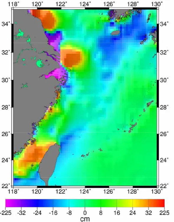
Fig. 4 shows the tidal height differences between the NAO tide (Mastsumoto et al., 2000) and the CSR4.0 tide (Eanes, 1999) at a selected epoch. Again, large tidal height differences occur in the same places where large standard errors of SSHs (Fig. 3) and large gravity anomaly differences (Fig. 2) occur, showing these three quantities are geographically correlated. The NAO and CSR4.0 tide models are derived from the TOPEX/Poseidon (T/P) altimeter data. Over areas with bad T/P SSHs , which are caused by bad range measurements and bad geophysical corrections, these two tide models will produce inaccurate tidal heights. Also, shallow-water tidal constituencies are not included in the models, adding to the tidal model errors. Those areas with large differences in Fig. 4 are just where NAO and CSR4.0 produce inaccurate tidal heights. Use of these inaccurate tidal heights to correct for the tidal effects in altimeter data will inevitably lead to degraded SSHs, and in turn large standard errors as seen in Fig. 3. In conclusion, inferior altimeter range measurements and inferior geophysical corrections combine to yield inferior SSHs, which in turn result in degraded gravity anomalies.

Over the ECS and the TS, the tidal amplitudes and phases have a complex pattern with short-period spatial variations (Jan et al., 2004; Lefevre et al., 2000). The strong, fast-changing tidal currents over the TS also increase the roughness of the sea surface and in turn increase the noise level of altimeter ranging (Sandwell and Smith, 2001. p. 444). This explains why the tide model error over the TS is large throughout the entire area (Fig. 4). In addition, the monsoonal winds in winter and summer induce large waves over the ECS and the TS (Jacobs et al., 2000; Wang, 2004), resulting in a rough sea surface for more than half of a year here. Therefore, one would expect that the noise level of altimeter measurement in these two areas is higher than that over a calm sea.

3. Data for gravity determination over shallow waters

3.1 Deflection of the vertical, differenced height and height slope

The basic observable of satellite altimetry is SSH, which is computed as the difference between satellite’s ellipsoidal height and the height above sea level measured by an altimeter. However, SSH is not the only data type that can be used for gravity derivation. A data type is along-track deflection of the vertical (DOV). For example, DOV has been used by Sandwell and Smith (1997) and Hwang et al. (2002). It has been shown that use of DOV can reduce the effect of long wavelength errors in altimeter data (Sandwell and Smith, 1997; Hwang, 1997). Typical long wavelength errors are orbit error and ocean tide model error. Along-track DOV is defined as

s h ∂ ∂ − = ε (1)

where h is geoidal height obtained by subtracting the dynamic ocean topography from SSH, and s is the along-track distance. Since h is discretely sampled, DOV in (1) can

(7)

only be approximately computed. On the other hand, differenced height is free from approximation. A differenced height is defined as

i i

i h h

d = ₊₁− (2)

where i is index of an SSH observable. Using differenced height has the same advantage as using along-track DOV in terms of mitigating long wavelength errors. A data type similar to differenced height is height slope, defined as

i i i i s h h − = +1 χ (3)

where is the distance between the points associated with . The spectral characteristics of height slope are the same as DOV and gravity anomaly, because they are all the first spatial derivatives of the Earth’s disturbing potential. Again, the advantage of using height slope is similar to that of using differenced height in mitigating altimeter data errors.

i i i g h h d g − (5)

(6) cov

Finally, the covariance function between gravity anomaly and height slope is

(

i i i g d s g, ) 1 cov , cov(∆ χ = ∆

)

(7)

(8)

function between two heights and the covariance function between gravity anomaly and height. General methods to model these two covariance functions can be found in Tscherning and Rapp (1974) and Moritz (1980). In this paper, we use the Model 4 gravity anomaly variance of Tscherning and Rapp (1974) to compute the needed covariance functions, see also Hwang and Parsons (1995). Furthermore, we used the remove-restore procedure with the EGM96 model (Lemoine et al., 1998) as the reference gravity field.

The general expression of LSC for altimeter-gravity conversion is

(

C C

)

l C ∆g 1 n t sl − + = (8)

where vector l contains any data related to the Earth’s disturbing potential, and

are the signal and noise parts of the covariance matrices of l, and is the covariance matrix of gravity anomaly and the signal of l. Altimeter data can also be used to compute geoidal undulation: one simply replaces by the covariance matrix of geoid- signal of l in (8). Note that the correlation between two successive DOVs, differenced heights or height slopes along the same satellite pass is -0.5, which must be included in .

t C C_n sl C sl C n C 3.2 Use of coastal land data

In theory, converting one functional of the Earth’s gravity field to another requires data on the whole Earth. Use of a reference gravity field may eliminate such a need. However, in the immediate vicinity of a computational point, data are needed in all directions. This condition cannot be met in the coastal area. Therefore, altimeter-gravity conversion near coasts is equivalent to an extrapolation process. This problem can only be mitigated using land data near the coasts. For example, land gravity anomalies and DOVs determined from astro-geodetic observations are such data. Another type of data is geoidal height obtained from Global Positioning System (GPS)-derived ellipsoidal height and orthometric height from precision leveling. That is,

H h

N = − (9)

where N, h and H are geoidal height, ellipsoidal height and orthometric height, respectively. Due to the need in engineering and mapping applications, geoidal heights from GPS and leveling could be abundant in coastal areas, especially those with dense populations. Methods to combine altimeter data and land data for gravity determination are, e.g., LSC and the input-output system method (Li and Sideris, 1997). The usefulness of land data in enhancing the accuracy of altimeter-derived gravity anomaly will be demonstrated in Section 5.2.

(9)

Altimeter-gravity conversion requires careful processing of altimeter data. Here we investigate the issue of outlier detection. Outliers in altimeter data will create a damaging effect on the resulting gravity fields. Methods for removing outliers in one-dimensional time series are abundant in the literature, e.g., Kaiser (1999), Gomez et al. (1999) and Pearson (2002). In this paper, we will use an iterative aaproach to remove outliers in along-track altimeter data. Consider a time series of along-track altimeter observable with the along-track distance as the independent variable. First, a filtered time series can be obtained by convolving the original time series with the Gaussian function 2 2 ) ( σ x e x f − = (10)

where x is the distance between two data points and σ is the 1/6 of the given window size of convolution. A window size is the length of a window within which all data points are convolved with the Gaussian function. The definition of the Gaussian function in (10) is the same as that defined in module “filter1d” of GMT (Wessel and Smith, 1995). For all data points the differences between the original and the filtered values are computed, and the standard deviation of such differences is determined. The largest difference that also exceeds three times of the standard deviation is considered an outlier and the corresponding data value is removed from the time series. The cleaned time series is filtered again and the new differences are examined against the new standard deviation to remove remaining outliers. This process is repeated and terminates when no outlier is found.

We tested this outlier detection method using altimeter data from the repeat and non-repeat missions. The altimeter data type used is differenced height. It turns out outliers in differenced heights are very sensitive to this method, especially when along-track SSHs experience an abrupt change. A spike of SSH will translate into two large height differences. As an example, Fig. 5 shows the result of outlier detection along two tracks of Geosat/ERM. In this case, the outliers are removed using a 28-km window size to generate the filtered time series (see (10)). Another test was carried out using data from a non-repeat mission--Geosat/GM. Fig. 6shows the result of the test along two tracks of Geosat/GM. In this case, we used an 18-km window size. According to our experiments, different window sizes for outlier detection should be used for altimeter data from different missions. Based on numerous tests, in this paper we adopt 28 km and 18 km as the optimal window sizes for the repeat and non-repeat missions, respectively, over the ECS and the TS.

(10)

5.1 The East China Sea

The first case study using the three altimeter data types and our outlier detection method was carried out in the ECS. The altimeter data we used are from the non-repeat missions ERS-1/GM and Geosat/GM, and the repeat missions Geosat/ERM, ERS-1/35-day, ERS-2/35-day and TOPEX/Poseidon 10-day repeats. Estimated uncertainties of these data are also available for use in LSC (see (8)). All altimeter data were screened against outliers using differenced heights. Fig. 7 shows the distribution of data outliers from all altimeter missions in the ECS and the TS. Fig. 7 shows that outliers could happen anywhere in the oceans. Clusters of outlier occur near coastal areas spotted with small islands, e.g., a spot off the southwestern coast of Korean and a spot near the Yangtze River. Clusters of outlier are also found along the Ryukyu Island Arc.

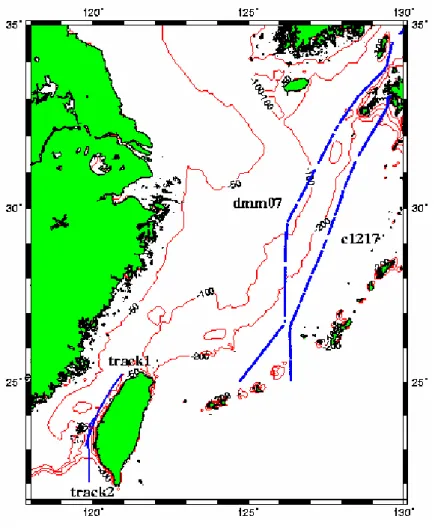
We experimented with four cases of altimeter-gravity conversion. In these four cases, we use two methods of conversion: LSC and the inverse Vening Meinesz method (Hwang, 1998), and three altimeter data types: DOV, differenced height and height slope. To identify the best case, we compared the altimeter-derived gravity anomalies with shipborne gravity anomalies. Fig. 8shows the tracks of two selected cruises in the ECS and another two tracks in the TS. Table 2 shows the statistics of differences between the altimeter-derived and shipborne gravity anomalies. The best result is from the case of using LSC with differenced height, followed by the case of using LSC with height slope. The case of using LSC with DOV yields the least accurate gravity anomalies.

To see the possible sources causing the differences between altimeter-derived and shipborne gravity anomalies, we computed the normalized values of gravity anomaly differences (Case 1 gravity anomaly vs. shipborne gravity anomaly), depths, standard errors of ERS-1 SSH, tidal height differences (CSR4.0 vs. NAO 99) along Cruises c1217 and dmm07 (Fig. 9). A normalized value, y, is obtained by

x x x y σ − = (11)

where x is the raw value,x is the mean value, σ_xis the standard deviation of the time series. As seen in Fig. 9, the gravity anomaly differences fluctuate rapidly and do not possess a particular pattern with respect to the other three quantities. Over the shallow waters (depth <100 m) of the ECS, both gravity anomaly differences and tidal height differences are relatively large. In general, the standard error of ERS-1 SSH increases with decreasing depth. Furthermore, the tidal height difference is larger over shallow waters than over the deep waters, and this agrees with the conclusion drawn in Section 2.

(11)

5.2 The Taiwan Strait

Next we carried out experiments in the TS using the same four cases as in the ECS. As shown in Fig. 7, outliers occur over areas near and away from the coasts and there is no particular pattern in the outlier distribution. We use shipborne data along two selected cruises to evaluate the altimeter-derived gravity anomalies. These shipborne gravity data were provided by Hsu et al. (1998). Table 3 shows the results of the comparisons between altimeter-derived and shipborne gravity anomalies in the four cases. The conclusion from Table 3 is similar to that from Table 2, except that the case of using the inverse Vening Meinesz method with DOVs produces the worst result. Therefore, over the ECS and TS, differenced height is the best data type for gravity derivation provided that the same conversion method is used.

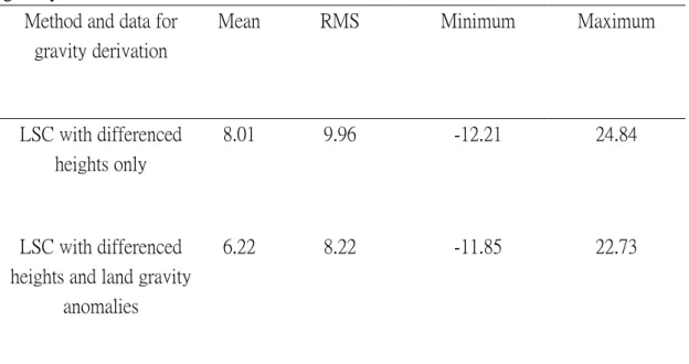
Since land gravity data are available near the TS, we also investigated the impact of land gravity data on altimeter-derived gravity anomalies. Fig. 10 shows the distribution of land gravity and altimeter data around Taiwan. As seen in Fig. 10, there is no altimeter over the immediate coastal waters off the coasts of Taiwan, where altimeter-derived gravity anomalies may contain large uncertainties. For the investigation, we experimented with the method of LSC using differenced heights, and with and without land gravity data (two cases). Table 4 shows the results of the comparisons between altimeter-derived and shipborne gravity anomalies. Clearly the accuracy of altimeter-derived gravity anomalies has been improved by including land gravity data.

Again, we investigated the possible causes of the difference between altimeter-derived and shipborne gravity anomalies in the TS. Fig.11 shows the same quantities as in Fig. 9, but in the TS. Again, along the two ship tracks, the patterns of gravity anomaly difference are quite random and are not correlated with depth and tidal height difference. However, there is a strong correlation (about 0.9) between standard error of ERS-1 SSH and tidal height difference along both Tracks 1 and 2. Again, tidal height difference increases as decreasing depth.

The conclusions from the analyses associated with Figs. 9 and 11 are in agreement with the conclusion drawn in Section 2: the major source of large standard error of SSH and large error of altimeter-derived gravity anomaly is tide model error. Another cause of degraded altimeter-derived gravity anomaly near coasts, which is not investigated in this paper, is low altimeter data density due to data editing. Even the data editing criterion near coasts is relaxed to increase data density, the additional altimeter data may not be of good quality for gravity derivation. One way to improve altimeter data quality near coasts is to retrack waveforms of altimeter ranging. For example, Deng et al. (2003) have obtained improved T/P SSHs by waveform retracking over Australian coasts. Here we suggest a procedure to improve the accuracy of altimeter-derived gravity anomalies:

(12)

(1) retrack near-shore waveforms of altimeter to produce waveform-corrected SSHs, (2) use the corrected SSHs to improve tide model, (3) use improved tide model to correct for the ocean tide effect in SSH. Finally, improved SSHs are used to determine improved gravity anomalies.

6. Conclusions

This paper studies the sources of large differences among three existing global gravity anomaly grids over the ECS and the TS. We conclude that tide model error is the biggest contributor to the large differences. Also, the complicated sea states in these two areas increase the roughness of the sea surface and the noise level of altimeter ranging. We experimented with two new altimeter data types: differenced height and slope. Use of LSC with differenced height produces the best result compared to other cases. Under the same conversion procedure, differenced height is the best altimeter type for gravity derivation. The differences between altimeter-derived and shipborne gravity anomalies were investigated. It is found that tide model error and standard error of SSH are correlated. For future work, it is suggested to retrack altimeter waveforms for increasing altimeter data density and quality near coasts. Currently, global retracked ERS-1 and Geosat waveforms are available (Lillibridge et al., 2004; Smith et al., 2004), and have been shown to produce improved marine gravity fields. Use of difference height from retracked altimetry (Case 1 in Section 5) for gravity derivation will be a subject of investigation in future studies.

References

Andersen, O.B., Knudsen, P., 2000. The role of satellite altimetry in gravity field modeling in coastal areas. Phys. Chem. Earth (A) 25 (1), 17-24.

Andersen, O.B., Knudsen, P., Trimmer, R., 2005. Improved high resolution altimetric gravity field mapping (KMS2002 global marine gravity field). Proc., IAG Symposia, Vol. 127, IUGG Sapporo, 2003, Springer, Berlin.

Fu, L.-L, Cazenave, A. (Eds.), 2001. Satellite Altimetry and Earth Sciences: A Handbook of Techniques and Applications. Academic Press, San Diego.

Cazenave, A., Royer, J.Y., 2001. Applications to marine geophysics. In Fu, L.L., Cazenave, A., Satellite Altimetry and Earth Sciences: a Handbook of Techniques and Applications. Academic Press, San Diego.

Deng, X., Featherstone, W.E., Hwang, C., Berry, P.A.M., 2003. Estimation of contamination of ERS-2 and POSEIDON satellite radar altimetry close to the coasts of Australia. Mar. Geod. 25, 189-204.

Eanes, R., 1999. Improved ocean tide model from satellite altimetry. Fall Meeting 1999. Am. Geophys. Un., San Francisco.

Gomez, V., Maravall, A., Pena, D., 1999. Missing observations in ARIMA models: skipping approach versus additive outlier approach. J. Econo. 88 (2), 341-363.

(13)

Hipkin, R., 2000. Modeling the geoid and sea-surface topography in coastal areas. Phys. Chem. Earth (A) 25 (1): 9-16.

Hsu, S., Liu, C., Shyu, C., Liu, S., Sibue, J., Lallemand, S., Wang, C., Reed, D., 1998. New gravity and magnetic anomaly maps in the Taiwan-Luzon region and their preliminary interpretation. Terr. Atm. Ocean. 9(3), 509-532.

Hwang, C., Parsons, B., 1995. Gravity anomalies derived from Seasat, Geosat, ERS-1 and Topex/Poseidon altimeter and ship gravity: a case study over the Reykjanes Ridge. Geophys. J. Int. 122, 551-568.

Hwang, C., 1997. Analysis of some systematic errors affecting altimeter-derived sea surface gradient with application to geoid determination over Taiwan. J. Geod. 71, 113-130.

Hwang, C., 1998. Inverse Vening Meinesz formula and deflection-geoid formula: applications to the predictions of gravity and geoid over the South China Sea. J. Geod.72, 304-312.

Hwang, C., Hsu, H.Y., Jang, R., 2002. Global mean sea surface and marine gravity anomaly from multi-satellite altimetry: applications of deflection-geoid and inverse Vening Meinesz formulae. J. Geod. 76, 407-418.

Hwang, C., Hsu, H.Y., Deng, X., 2004. Marine gravity anomaly from satellite altimetry: a comparison of methods over Shallow Waters. In Hwang, C., Shum, C., Li, J.C.., Satellite Altimetry for Geodesy, Geophysics and Oceanography. International Association of Geodesy Symposia, 126, 59-66, Springer, Berlin.

Hwang, C., Shum, C.K. and Li, J.C. (Eds.), 2004. Satellite Altimetry for Geodesy, Geophysics and Oceanography. International Association of Geodesy Symposia, 126, Springer, Berlin.

Jacobs, G.A., Hur, H.B., Riedlinger, S.K., 2000. Yellow and East China Seas response to winds and currents. J. Geophys. Res.105 (C9), 21947-21968.

Jan, S., Chern, C.S., Wang, J., Chao, S.Y., 2004. The anomalous amplification of M-2 tide in the TS. Geophys. Res. Lett. 31 (7), Art. No. L07308.

Kaiser, R., 1999. Detection and estimation of structural changes and outliers in unobserved components. Comp. Stat. 14 (4), 533-558.

Lefevre, F., Le Provost, C., Lyard , F.H., 2000. How can we improve a global ocean tide model at a regional scale? A test on the Yellow Sea and the East China Sea. J. Geophys. Res. 105 (C4), 8707-8725.

Lemoine, F.G., Kenyon, S.C., Factor, J.K., Trimmer, R.G., Pavlis, N.K., Chinn, D.S., Cox C.M., Klosko, S.M., Luthcke, S.B., Torrence, M.H., Wang, Y.M., Williamson, R.G., Pavlis, E.C., Rapp, R.H., Olson, T.R., 1998. The Development of Joint NASA GSFC and the National Imagery and Mapping Agency (NIMA)

(14)

Geopotential Model EGM96. Rep NASA/TP-1998-206861, National Aeronautics and Space Administration, Greenbelt, MD

Li, J., Sideris, M., 1997. Marine gravity and geoid determination by optimal combination of satellite altimetry and shipborne gravimetry data. J. Geod. 71, 209-216.

Lillibridge, J.L., Smith, W.H.F, Scharroo, R., Sandwell, D.T., 2004. The Geosat geodetic mission twentieth anniversary edition data product. AGU 2004 Fall meeting, San Francisco.

Matsumoto, K., Takanezawa, T., Ooe, M., 2000. Ocean tide models developed by assimilating TOPEX/Poseidon altimeter data into hydrodynamical model: a global model and a regional model around Japan. J. Oceanogr. 5, 567-581.

Moritz, H., 1980. Advanced Physical Geodesy, Herbert Wichmann, Karlsruhe.

Niwa, Y., Hibiya, T., 2004. Three-dimensional numerical simulation of M-2 internal tides in the East China Sea. J. Geophys. Res. 109 (C4), Art. No. C04027.

Pearson, R.K., 2002. Outliers in process modeling and identification. IEE Trans. on Control Tech. 10, 55-63.

Rapp, R., Balasubramania, N., 1992. A Conceptual Formulation of a World Height System. Rep. No. 421, Dept. of Geod. Sci. and Surveying, Ohio State University, Columbus, Ohio.

Sandwell, D.T., Smith, W.H.F., 1997. Marine gravity anomaly from Geosat and ERS-1 satellite altimetry. J. Geophys. Res. 102 (B5), 10039-10054.

Smith, W.H.F., Sandwell, D.T., 2004. Improved global marine gravity field from reprocessing of Geosat and ERS-1 radar altimeter waveforms. AGU 2004 Fall meeting, San Francisco.

Tscherning, C.C., and Rapp, R.H., 1974. Closed Expressions For Gravity Anomalies, Geoid Undulations And Deflection Of The Vertical Implied By Anomaly Degree Variance Models. Rep. 208, Dept. of Geod. Sci. and Surveying, Ohio State University, Columbus, Ohio.

Wang, C.K., 2004. Features of monsoon, typhoon and sea waves in the Taiwan Strait. Mar. Geores. & Geotech. 22 (3), 133-150.

Wessel, P., Smith, W.H.F., 1995. New version Generic Mapping Tools release, EOS Trans. AGU, 76.

Yanagi, T., Morimoto, A., Ichikawa, K., 1997. Seasonal variation in surface circulation of the East China Sea and the Yellow Sea derived from satellite altimetric data. Cont. Shelf Res. 17 (6), 655-664.

(15)

Table 1: Statistics of the differences among the NCTU02, SS02 and KMS02 global gravity anomaly grids over the area 118°−130°E,22°−35°N

(a) NCTU02-SS02 Depth (m) 0-100 100-200 200-500 > 500 Mean (mgal) 0.14 0.330 0.22 0.08 RMS (mgal) 6.35 10.10 5.81 7.86 No. of points 50491 14964 7426 39450 (b) NCTU02-KMS02 Depth (m) 0-100 100-200 200-500 > 500 Mean (mgal) -0.12 0.27 -0.34 -0.03 RMS (mgal) 6.86 9.90 6.45 7.97 No. of points 50491 14964 7426 39450 (c) KMS02-SS02 Depth (m) 0-100 100-200 200-500 > 500 Mean (mgal) 0.27 0.05 0.56 0.12 RMS (mgal) 4.96 4.06 5.65 4.21 No. of points 50491 14964 7426 39450

Table 2: Statistics of differences (in mgals) between altimeter-derived and shipborne gravity anomalies in East China Sea

Case Mean RMS Min Max

LSC with differenced height

-5.33 13.02 -49.24 43.96

LSC with height slope -5.45 13.19 -50.77 44.38 LSC with DOV -4.61 16.99 -85.59 74.65 Inverse Vening Meinesz

with DOV

-4.11 15.53 -52.23 80.53

(16)

Table 3: Statistics of differences (in mgals) between altimeter-derived and shipborne gravity anomalies in Taiwan Strait

Case Mean RMS Minimum Maximum

LSC (differenced height) 7.09 9.06 -8.92 23.56

LSC (height slope) 7.94 10.26 -9.39 28.96

LSC (DOV) 7.70 10.44 -10.97 29.38

Inverse Vening Meinesz (DOV)

7.59 10.73 -14.88 29.37

Table 4: Statistics of difference (in mgals) between altimeter-derived and shipborne gravity anomalies in the Taiwan Strait

Method and data for gravity derivation

Mean RMS Minimum Maximum

LSC with differenced heights only

8.01 9.96 -12.21 24.84

LSC with differenced heights and land gravity

anomalies

(17)

Fig. 1: Bathymetry (dashed lines) and distribution of shipborne gravity data (dots) in the East China Sea and Taiwan Strait.

(18)

Fig. 2: Differences between NCTU02, SS02 and KMS02 global gravity anomaly grids.

(19)

Fig. 3: Standard errors of sea surface heights from the Geosat/ERM, ERS-1/35 day and ERS-2/35 day repeat missions.

(20)

Fig. 4: Tidal height difference between the NAO and CSR4.0 tide models at a selected epoch.

(21)

Fig. 5: (a) Ascending and descending passes of Geosat/ERM for outlier detection, (b) results with a with a 28-km window size. Outliers are not connected by the lines.

(a)

(b)

(22)

Fig. 6: (a) Ascending and descending passes of Geosat/GM for outlier detection, (b) results with a 18-km window size. Outliers are not connected by the lines.

(a)

(b)

(23)

(24)

Fig. 8: Distribution of shipborne gravity anomalies in the East China Sea and the Taiwan Strait for comparison with altimeter-derived gravity anomalies.

(25)

Fig. 9: Time series of normalized difference of gravity anomaly, standard error of ERS-1 SSH, tide model difference and depth, along Cruise dmm07 (top) and c1217.

(26)

(27)

Fig. 11: Time series of normalized difference of gravity anomaly, standard error of ERS-1 SSH, tide model difference and depth, along Track 1 (top) and Track 2.

(28)

PART II: Coastal gravity anomaly from retracked Geosat/GM

altimetry: improvement, limitation and the role of airborne gravity

data

1. Introduction

Most marine applications of satellite altimetry begin with sea surface height (SSH). A sea surface height of altimetry is derived from the satellite’s orbital height and the range between the antenna and the sea determined using the waveforms of the altimeter. Over the deep ocean without land interference, the waveforms created by the returning altimeter pulse in general follow the ocean model of Brown (1977) and the corresponding range can be properly determined using the result from an onboard tracker. Near coasts or over waters with obstacles, where the waveforms may be corrupted due to a variety of reasons, range observations can be in error. For example, such corruptions of waveforms in the ERS and Envisat altimetry over the world coastal zones have been presented by Mathers et al. (2004). Use of erroneous altimeter ranges may lead to false results in such applications as gravity anomaly determination and sea level change study. Recent efforts by, e.g., Smith and Sandwell (2004) and Andersen et al. (2005), have shown that use of retracked SSHs can improve the determination of gravity anomaly over coastal waters and the open ocean. A retracked SSH here is defined as a SSH which is, in addition to standard geophysical and instrument corrections (Fu and Cazenave, 2001), corrected by the tracking gate bias determined from waveform retracking. Altimeter waveform corruption can be in various forms, depending on the altimeter and the geographic location. For example, Deng et al. (2002) estimated that TOPEX/Poseidon (T/P) waveforms are corrupted over waters about 20 km to the shore around the southern Australia. Waveform corruptions over ice and land are in different patterns than those over coastal waters, requiring different algorithms for proper retracking.

Methods of waveform retracking may be classified into two categories: one is based on functional fit and the other based on statistics. A review of waveform retracking methods can be found in, e.g., Deng (2004) and Zwally and Brenner (2001). The goal of this study to is develop an improved method for retracking Geosat/GM altimeter waveforms and assess the extent of improvement that this method can achieve. We will focus on just one recipe of retracking based on our available resources, and we have no intention to assess the performances of all retrackers available in the scientific community. As an application of the retracked Geosat/GM altimetry, gravity anomaly will be derived from retracked SSHs of Geosat/GM and its quality will be assessed.

The area chosen for the experiments in this paper is over the waters around Taiwan. The bathymetry and coastal geometry here are rather diversified (Fig. 1). East of Taiwan,

(29)

the collision of the Eurasia Plate and the Philippine Sea Plate creates islands and complex shorelines. Here the depth of the Pacific Ocean plunges to 4 km just about 10 km to 20 km off the east coast of Taiwan. West of Taiwan lies the Taiwan Strait, where the deepest part is only 50 m and the waters is scattered with islands and barrier islands. Less than 200 m in depth, the East China Sea lies north of Taiwan and is also scattered with islands near Taiwan. The South China Sea is situated south of Taiwan and here a small island called Liuchou might interfere with altimeter waveforms. Given the varying depths and the complicated coastal geometry around Taiwan, different degrees of waveform corruption will be expected. In addition, the roughness of the gravity field around Taiwan varies from one area to another: it is smooth over the Taiwan Strait, the East China Sea and the South China Sea (range of gravity anomaly variation: tens of mgal) and it is rough over the Pacific Ocean (range of gravity anomaly variation: hundreds of mgal). Ocean tides in the Taiwan Strait are complicated, with large tidal amplitudes near the coasts of the mainland China and Taiwan (Jan et al., 2004). Here we would expect large remaining errors in altimetry due to tide model error, even after altimeter ranges are properly corrected by retracking.

The well edited shipborne gravity data from Hsu et al. (1998) will make it possible to assess the accuracy of altimeter-derived gravity anomalies around Taiwan. Furthermore, airborne gravity data are available here (Hwang et al., 2005) and can be used to see (1) whether adding airborne gravity data to altimeter data will enhance the accuracy of altimeter-derived gravity anomaly, and (2) to assess the accuracy of altimeter-only gravity anomaly over regions of different depths, including the immediate vicinity of coasts.

2. Geophysical and waveform data records of Geosat/GM

The data needed for this work are the data products of the Geosat/GM mission, including the Geophysical Data Records (GDRs), Sensor Data Records (SDRs) and Waveform Data Records (WDRs) of the Geosat/GM satellite mission. These data were supplied by the National Oceanic and Atmospheric Administration (NOAA); see also Cheney et al. (1991) and Lillibridge et al. (2004) for the descriptions of Geosat GDRs, SDRs and WDRs. One day of Geosat/GM GDRs are stored in one file and the data set spans from day 90 of 1985 to day 273 of 1986, resulting in a total of 549 days and files. In one GDR record, there are 78 bytes of information containing 34 parameters, including geophysical corrections at 1 Hz. Near coasts and over land, missing GDRs are frequent due to loss of lock of altimeter. In contrast, half day of WDRs are stored in one file. Each WDR contains 660 bits of information, including waveforms at 10 HZ.

The SDR product contains the raw measurements and on-board computed parameters. Each SDR also spans a 24-hour measurement period from midnight to

(30)

midnight (cf. Cole, 1985). In contrast, half day of WDRs are stored in one file. Each WDR contains 660 bytes of information, but only including radar return waveform samples for each of the 63 altimeter gates at 10 HZ. The GDR, SDR and WDR data products require ancillary information which is applicable to the entire data span. Such information used in this study is the time measurements. The time format associated with a GDR is Coordinated Universal Time (UTC), while a Geosat-A Telemetry Stream time format is associated with both the SDR and WDR. Following the telemetry stream definition a frame count (FC) is computed as

mFC MFC

32

FC= × + _（1）

where MFC is the major frame count and mFc is the minor frame count, both available on SDRs and WDRs. In this paper, we convert UTC of GDR to FC as

⎟⎟ ⎠ ⎞ ⎜⎜ ⎝ ⎛ ₊ ₋ = 4.4 sec_per_fc 0.005 -epoch_s85 -s85 0 FC int FC_GDR (2)

where FC_GDR is the FC associated with a UTC ( ), int stands for the integer part, is the beginning count of FC in a day, is 0 hour UTC of a day and is the time span of a FC. This result in a consistent time frame for properly extracting geophysical corrections and other information from GDRs, which are then combined with the range corrections from the retracking of waveforms in WDRs. The geophysical corrections applied to Geosat/GM instantaneous SSHs in this paper are the same as those described in Hwang at al. (2002).

s85 FC0 epoch_s85 sec_per_fc

3. Retracking Geosat/GM waveforms

3.1. Selected methods of waveform retracking

Waveforms are a series of powers at altimeter gates generated by a returning pulse of altimeter from the sea. In the open ocean, waveforms are assumed to follow the functional form of Brown (1977) and the corresponding range between the antenna and the sea is derived from an onboard tracker based on such waveforms. The tracker works in a window of waveforms. The tracking gate within the window determines the time for calculating the range. For the ocean mode, the tracking gate is set to be at the center point of the leading edge. For example, Fig. 2 shows typical waveforms of Geosat over the open ocean and the tracking gate is assumed to be 30.5. As the altimeter approaches land, the surface geometry and reflecting properties begin to deviate from those over the open ocean, leading to distorted waveforms. Fig. 3 shows waveforms of Geosat as the

(31)

altimeter passed over the Peng-Hu Island in the Taiwan Strait. In Fig. 3, there are two leading edges (ramps) in the waveform. Clearly the pre-defined tracking gate is not at either of the center points of the two leading edges. Waveforms like those given in Fig. 3 will have to be retracked in order to determine the proper tracking gate (called retracking gate) and hence the correct range.

There are numerous methods for waveform retracking. In this paper, we will experiment with four methods that are both based on functional fit and statistics. For the method of functional fit, we chose to use the Beta-5 retracker (Martin et al., 1983; Anzenhofer et al., 1999), which fits waveforms by the function

(

)

_⎟⎟ ⎠ ⎞ ⎜⎜ ⎝ ⎛ − + + = 4 3 5 2 1 1 _β β β β β Q p t y_t （3） with

(

₃ ₄

)

₃3 0.5 ₄4 5 . 0 5 . 0 0 β β β β β β ≥ + + < ⎩ ⎨ ⎧ + − = t for t for t Q （4）

( )

_∫

₋_∞ _⎟⎟ ⎠ ⎞ ⎜⎜ ⎝ ⎛ − = x q dq x p 2 exp 2 1 2 π （5）

wherey_t is the power at gate t (t ranges from 1 to 60 for Geosat),

β

₁ is thermal noise,

2

β

is the amplitude,

β

β

in eq. (3)). In this method, we have excluded powers at the first and last n gates (n is set to 4 in this paper), which might contain large noises and damage the solution. The estimates of waveform parameters from OCOG can be used as a priori values in the least-squares solution of the beta-5 retracker. It can also be used to classify waveforms and to estimate waveform quality (Anzenhofer et al., 1999). In comparison to the Beta-5 retracker, the OCOG retracker is easy to implement on a computer. While there is no guarantee of convergence in the least-squares solution of the Beta-5 retracker, the OCOG retracker will always deliver a solution.

Another statistics-based method to be assessed is a modified threshold retracking. This method employs a threshold value to determine the retracking gate. The formulae we use are

∑

= = 5 1 5 1 i i N y y （10）

(33)

(

N

)

N l A y y T =α − + (11) 1 1 − − + − = k k k thr y y G Gr Tl −yk−1 （12）

where A is determined by eq. (6), yNis the averaged value of the first five powers, αis a threshold value, is kth gate whose power is greater than , and is the

retracking gate (equivalent to

k G Tl r thr G 3

β

and ). If equals , then k is replaced by k+1. Using

r ocog

G y_k yk−1

α= 10%, 20%, 30% and 50%, we have done a number of tests to chose a properα . It turns out thatα =50% produces the best result over the ocean. The threshold retracking works well if the waveform contains just one ramp. However, if the waveforms contain more than one ramp (this often happens in coastal regions), the retracking gate is determined in favor of the leading edge of the first ramp and could lead to a false result.

3.2. An improved threshold retracking

In the case of complex waveforms, the threshold retracker cannot properly determine the center of the leading edge. In this paper we present an improved threshold retracker. Fig. 4 shows a flowchart of the improved threshold retracker, which determines one or more sub-waveforms and retracking gates, and then selects a best retracking gate according to the following procedure. First, the difference between the powers of every other two gates is computed. If half of the difference is greater than a given value ε₁, then it shows that the antenna begins to pick up the returning power. In this case (difference >ε₁), the difference between two successive powers is then computed. If this difference is greater than a given value ε₂, then it indicates that the antenna continues to pick up the returning power, and the corresponding gate and power are included in the first sub-waveform. The selection of sub-waveform gates is terminated when the difference is smaller than ε₂. Both ε₁ and ε₂ are determined empirically, and it is found that the result with ε₁ =8, andε₂ =2 is the best. The sub-waveform is then extended by including four gates at the beginning and the end of the sub-waveform. Using the selected samples in the sub-waveform, a retracking gate corresponding to this sub-waveform is determined using eqs. (6), (10), (11) and (12). This process is repeated for the next sub-waveform and a new retracking gate is determined. At the final step, we compare the previous SSH with the current SSHs associated with the computed retracking gates to make decision: the “best” retracking gate is the one that yields the smallest difference between the current SSH and the previous SSH. If the previous SSH is inadequate for comparison, the earlier SSH is

(34)

chosen. Since it is more likely that SSH can be accurately determined in the open ocean than in coastal waters, we always start the retracking from the open ocean and then proceed to the land. This is to ensure the criterion of SSH for the “best” retracking gate works properly. We do not compare a retracked SSH with an a priori SSH or a geoidal height, since there might be a bias between these two, which could lead to an incorrect retracking gate.

3.3. Results of waveform retracking around Taiwan

We have experimented with waveform retracking around Taiwan using the retrackers described above. One important issue is to find the optimal retracker for the subsequent gravity anomaly derivation. The selection of such a retracker is based on the following two criteria:

a）success rate of retracking, and

b）the standard deviation of the differences between the retracked SSHs and modeled geoid heights.

The geoid model for use in Criterion 2 is a gravimetric geoid model of Taiwan computed from the latest land/marine gravity data and airborne gravity data (Hwang et al., 2005). Because the assumption made in the OCOG retracker, it is only used for computing a priori values of the parameters needed in the other retrackers. Table 1 shows a typical comparison of retracked SSHs and geoidal heights along Geosat/GM track 85206 (data on day 206, 1985; see Fig. 5). In Table 1, we list the number of successfully retracked waveforms, the number of raw waveforms, the ratio between these two numbers and the standard deviation of the differences between retracked SSHs and geoidal heights for each retracker. Because of the complex waveforms near the coasts, the success rate of the Beta-5 retracker is only 70%. There is no problem of convergence for the threshold retracker, so its success rate is always 100%. The improved threshold retracker yields almost 100% of success rate. The standard deviations of the height differences in Table 1 are based on only retracked SSHs. Fig. 5 shows retracked SSHs and geoid heights along track 85206. The deviation of SSH from geoidal height increases as track 85206 approaches the land. In other tests that we have done, the Beta-5 retracker delivers success rates of retracking at about 70-80 %, which is considered inadequate for retracking around Taiwan. In terms of both success rate and standard deviation, Table 1 shows that the improved threshold retracker is significantly better than the other two retrackers. The results from other tests confirm that the improved threshold retracker indeed outperforms the other two retrackers, and hence it is selected as the optimal retracker in this paper.

The improved threshold retracker is further tested considering the dependency of retracking accuracy on region and depth. Fig. 6 shows the ground tracks of retracked

(35)

SSHs around Taiwan. In total, there are Geosat/GM 165 tracks here. The performance of the improved threshold retracker is assessed at four marine zones in Fig. 6 and at regions of different distances to the shores. Fig. 7 shows the distribution of the differences between retracked SSHs and geoidal heights. As seen in Fig. 7, retracking not only improves the accuracy of SSH over the coastal waters, but also over the open ocean. The places with most improved SSHs are near islands in the ocean and around barrier islands off the west coast of Taiwan. It is clear that not all SSHs can be properly corrected by retracking, as there are still remaining large errors seen in Fig. 7. This is a limitation of waveform retracking. These large errors may be caused by improper retracking and/or tide model error. Regarding tide model error, Hwang (1997) has assessed the accuracy of the CSR3.0 tide model around Taiwan and found that, the model error is the least (about few cm) in the Pacific Ocean east of Taiwan and the largest (about few decimeter) in the Taiwan Strait. At the central Taiwan Strait off the coasts of the mainland China and Taiwan, the tidal amplitude can reach 3 m. Here the difference in the M2 tide amplitude between CSR4.0 and observation is found to be about 50 cm. Efforts beyond waveform retracking for improving altimetry quality are presented in Anzenhofer et al. (1999).

The improvement percentage (IMP) of retracked SSHs is also computed, using

% 100 IMP raw retracked raw − × = σ σ σ （13）

where σRaw and σRetracked are the standard deviations of the differences between raw SSHs and geoidal heights, and retracked SSHs and geoidal heights, respectively. Table 2 shows the improvement percentages in four cases. A negative improvement percentage indicates that retracking deteriorates SSHs. Table 2 shows that the improvement percentage increases as the waters approaches the land. While the difference in the improvement percentage between the marine zones at 20 km and 10 km to the shores is only marginal, the difference in standard deviation is significant. The largest improvement is at Zone 1 and the least improvement is at Zone 4, irrespective of the distance to the shore. However, SSHs in Zone 2 are degraded by waveform retracking, with unknown reason.

4. Gravity anomalies from retracked Geosat/GM altimetry 4.1. Gravity anomaly derivation by least-squares collocation

We have experimented with two methods of gravity derivation from retracked SSHs of Geosat/GM. One is the inverse Vening Meinesz formula (Hwang, 1998) and the other is least-squares collocation (LSC) (Moritz, 1980; Hwang and Parsons, 1995). In all

(36)

experiments (Section 4.2), LSC always outperforms the inverse Vening Meinesz formula by few mgal in the accuracy of computed gravity anomaly. Thus, gravity derivations in Section 4.2 will be solely based on LSC. Furthermore, LSC is able to combine heterogeneous data for gravity anomaly derivation and this function is needed in our experiments. In all cases, the sea surface topography (SST) is regarded as zero, so that SSH is considered identical to geoidal height. In fact, there is no reliable estimate of SST around this region.

We used the standard remove-restore procedure in the LSC derivation of gravity anomaly. Along-track geoid gradient derived from SSH is used as data type. The adopted reference gravity field is a combined gravity field from the GRACE GGM02C model (degrees 2 to 200; GRACE home page) and the EGM96 model (degrees 201 to 360; Lemoine et al., 1998). First, a residual geoid gradient is computed by

long

res e e

e = − （14）

where , and are observed, long wavelength and residual gradients,

respectively. The residual gravity anomaly is computed by the standard LSC formula with geoid gradients as input (Hwang and Parsons, 1995):

e elong eres

(

)

res 1 nn ee ∆ge C C e C + − = ∆g_res （15） where is a vector of residual geoid gradients, , and are covariance

matrices for gravity anomaly-gradient, gradient-gradient and noise of gradient, respectively. is a diagonal matrix holding the noise variances of geoid gradients. Based on numerous tests, it is found that a noise variance of 4 sec

res

e C∆ge Cee Cnn

nn C

2

for geoid gradient produces the best gravity anomaly. In the case of using combined altimeter and airborne gravimeter data, a residual gravity anomaly is computed by

(

)

_⎟⎟ ⎠ ⎞ ⎜⎜ ⎝ ⎛ ⎟⎟ ⎠ ⎞ ⎜⎜ ⎝ ⎛ + + = ∆ − res ar 1 nn ee e∆∆g e ∆g mm ∆g ∆ge ∆g∆g e ∆g C C C C C C C C ar a a res g (16)

where is a vector of residual airborne gravity anomalies, , , and

are covariance matrices for airborne gravity anomaly-gradient, gradient-gravity

anomaly, and gravity anomaly-airborne gravity anomaly, respectively, and is a diagonal matrix holding the noise variances of airborne gravity anomalies. In this paper,

ar ∆g C∆gae Ce∆∆g a ∆g∆g C mm C

(37)

a noise variance of 9 mgal2 is used in (Hwang et al., 2005).The LSC method in eq. (16) combines downward continuation, altimeter-to-gravity conversion and interpolation in one step using proper covariance functions.All the needed covariance functions and matrices were constructed based on the error degree variances of the combined GGM02C-EGM96 gravity field and the Tscherning and Rapp (1974) Model 4 degree variance; see Hwang and Parsons (1995, Appendix A) for the detail of covariance modeling related to this work.

mm C

4.2. Results: comparison with shipborne and airborne gravity data

The purpose of experiments in this section is to see whether retracking improves the accuracy of altimeter-derived gravity anomaly and to see the role of airborne gravity data. We computed three sets of gravity anomaly (designated as computed gravity anomaly) by LSC using the following three data sets:

Data set 1: raw SSHs,

Data set 2: retracked SSHs, and

Data set 3: retracked SSHs and airborne gravity anomalies.

Note that SSHs have to be converted to along-track geoid gradients before computing gravity anomalies. The resulting gravity anomalies from the three data sets were then compared with shipborne gravity anomalies. The gravity anomalies derived from Data sets 1 and 2 were also compared with airborne gravity anomalies. The shipborne gravity anomalies are from Hsu et al. (1998) and have been carefully edited and crossover adjusted. The estimated uncertainties of the shipborne gravity anomalies depend on ship cruises and locations, and are about several mgal (Hsu et al., 1998). The airborne gravity anomalies are from Hwang et al. (2005) and were collected at an averaged altitude of 5156 m using a LaCoste and Romberg System II air/sea gravimeter. Based on the crossover analysis of Hwang et al. (2005), the estimated uncertainty of airborne gravity anomalies is about 3 mgal. The airborne gravity data were mostly collected along north-south and west-east going lines, which are spaced at 4.5 km and 20 km, respectively (Fig. 10). Note that the gravity signal at an altitude of 5156 m is attenuated and its spectral content is different from that at sea level.

Table 3 shows the statistics of the differences between the computed gravity anomalies (three data sets) and the shipborne gravity anomalies. As another independent assessment, Table 4 shows the statistics of the differences between the computed gravity anomalies (data sets 1 and 2) and the airborne gravity anomalies. For comparison with airborne gravity anomalies, the altimeter-derived gravity anomalies were upward continued to the flight altitude (5156 m) using a remove-restore procedure with the long wavelength part from the combined GGM02C and EGM96 gravity field, see also Hwang et al. ( 2005). To enhance the accuracy of the upward continuation, the land

(38)

gravity anomalies on Taiwan were incorporated with the altimeter-derived gravity anomalies. Both Tables 3 and 4 show that, use of retracked SSHs indeed improves the accuracy of gravity anomaly. The percentage of improvement by retracking in this case is 11%. Adding airborne gravity to retracked SSHs further improves the accuracy, and the improvement is about one mgal. Possible reasons for such a marginal improvement (one mgal) are (1) airborne gravity data provide additional information only at the wavelengths corresponding to the flight height, and (2) down continuation will enlarge the noises of airborne gravity anomalies at sea level. As such, the resulting gravity anomalies from combined altimetry and airborne data cannot achieve the same accuracy as the airborne gravity anomalies (3 mgal at the flight altitude).

Fig. 8 shows gravity anomalies derived from raw SSHs and retracked SSHs. Many gravity artifacts associated with the raw SSHs (Fig. 8a) have disappeared in the gravity field associated with the retracked SSHs (Fig. 8b). Examples of such changes can be found at, e.g., a spot northeast of Taiwan (here many islands exist) and a marine zone near the Peng-Hu Island (central Taiwan Strait) and the waters off the southwest coast of Taiwan. This pattern of gravity accuracy improvement is consistent with the pattern of SSH accuracy improvement seen in Fig. 7. Also, there are spots with gravity artifacts in the gravity field derived from the retracked SSHs, and these spots are coincident with the spots with large remaining errors in retracked SSHs.

Fig. 9 shows the distributions of the differences between computed gravity anomalies (three data sets) and shipborne gravity anomalies. The differences between Fig. 9a and Fig. 9b are consistent with the differences between Fig. 8a and Fig. 8b. These differences show the regions where SSHs receive corrections from retracking and the accuracy of gravity anomaly is improved. In Fig. 9b, some of the differences off the east coast of Taiwan at about 24.3 exceed 50 mgal. Here use of a better retracker than the improved threshold retracker is needed to correct for the errors, or these retracked SSHs will have to be removed.

N °

The differences between Fig. 9b and Fig. 9c show the effects of including airborne gravity data. Adding airborne gravity to retracked SSHs improves the accuracy of gravity anomaly at marine zones close to, but not limited to, the coasts. The area with the most improved accuracy is over the waters off the entire west coast of Taiwan, and the waters around the islands in the Pacific Ocean. The spot with excessively large errors in the altimeter-only gravity anomalies (at 24.3 off the east coast of Taiwan) also sees some reduction in the error by adding the airborne gravity data, but unfortunately some errors are enlarged.

N °

Fig. 10 shows the distributions of the differences between computed gravity anomalies (sets 1 and 2) and airborne gravity anomalies. Here we will just discuss the differences at sea. The difference between the computed and the airborne gravity

(39)

anomalies is a function of location, altimeter data density (Fig. 6), retracking quality (Fig. 7), and roughness of gravity (Fig. 1). The pattern of improvement of gravity anomaly accuracy by retracking in Fig. 10 is similar to that in Fig. 9, but Fig. 10 shows more detail of improvement at the immediate vicinity of the coasts and islands. Fig. 10b shows that, as in Fig. 9b, there are still large errors in altimeter-derived gravity anomalies even retracked SSHs are used. Therefore, for coastal gravity anomaly derivation, the best strategy will be to remove bad SSHs and then fill the gap by airborne gravity data.

5. Conclusions

This paper assesses the performances of selected waveform retrackers and presents the improved threshold retracker, which is considered the optimal one for the area under study. Waveform retracking has improved the accuracy of Geosat/GM altimetry, but the improvement is limited to the cases when the waveforms can be properly retracked. As such, some of the retracked SSHs still contain large errors that damage the results of their applications. Such remaining large errors normally occur over the waters around islands and at the immediate vicinity of the coast. Despite these limitations, retracking has been shown to improve the accuracy of Geosat/GM-derived gravity anomaly. Again, the extent of accuracy improvement of gravity is limited by the effectiveness of retracking. Inclusion of airborne gravity data to retracked Geosat/GM altimetry further improves gravity accuracy, especially over coastal waters.

There are other factors than waveform contamination that will affect the accuracy of altimeter-derived SSH (Anzenhofer et al., 1999). One important factor is tide model error. Applying bad tidal corrections to properly retracked SSHs will surely damage the results of altimetry applications. Thus, an important future work is to use retracked altimetry to improve tide model, especially around coastal waters. The ideal altimeter data for such work will not be Geosat/GM data, but will be repeat altimeter data from such missions as Geosat/ERM, ERS-1/2, TOPEX/Poseidon and Envisat, all requiring waveform retracking before use.

References

Andersen OB, Knudsen P, Berry PAM, Mathers L, Trimmer R, Kenyon S (2005) Initial results from retracking and reprocessing the ERS-1 geodetic mission altimeter for gravity field purposes, International Association of Geodesy Symposia 129: 1-5.

Anzenhofer M, Shum CK, Rentsh M (1999) Coastal Altimetry and Applications, Rep. No. 464, Dept Geod Sci and Surveying, Ohio State University, Columbus, Ohio. Brown GS (1977) The average impulse response of a rough surface and its applications.

(40)

IEEE Trans Ant Prop AP-25 (1): 67-74

Cheney RE, Emery WJ, Haines BJ, Wentz F (1991) Recent improvements in GEOSAT altimeter data. EOS 72（51): 577-580

Davis CH (1997) A robust threshold retracking algorithm for measuring ice-sheet surface elevation change from satellite radar altimeter. IEEE Trans on Geosci and Remote Sensing 35(4): 974-979

Deng X, Featherstone W, Hwang C, Berry P (2003) Waveform retracking of ERS-1. Mar Geod 25: 189-204

Deng X (2004) Improvement of geodetic parameter estimation in coastal regions from satellite radar altimetry. PhD thesis, Curtin University, Australia

Fu LL, Cazenave A (2001) Satellite Altimetry and Earth Sciences: A Handbook of Techniques and Applications. Academic Press, San Diego

GRACE home page: http://www.csr.utexas.edu/grace/.

Hsu S, Liu C, Shyu C, Liu S, Sibue J, Lallemand S, Wang C, Reed D (1998) New gravity and magnetic anomaly maps in the Taiwan-Luzon region and their preliminary interpretation. Terr Atm Ocean 9(3): 509-532

Hwang C (1997) Analysis of some systematic errors affecting altimeter-derived sea surface gradient with application to geoid determination over Taiwan. J Geod 71: 113-130

Hwang C, Parsons B (1995) Gravity anomalies derived from SEASAT, GEOSAT, ERS-1 and TOPEX/Poseidon altimeter and ship gravity: a case study over the Reykjanes Ridge. Geophys J Int 122: 551-568

Hwang C (1998) Inverse Vening Meinesz formula and deflection-geoid formula: applications to the predictions of gravity and geoid over the South China Sea. J Geod 72: 304-312

Hwang C, Hsu HY, Jang RJ (2002) Global mean sea surface and marine gravity anomaly from multi-satellite altimetry: applications of deflection-geoid and inverse Vening Meinesz formulae. J Geod 76: 407-418

Hwang C, Hsiao YS, Shih SC, Yang M, Chen KH, Forsberg R, Olesen A (2005) Geodetic and geophysical results from the airborne gravity survey of Taiwan. submitted to J Geophys Res

Jan S, Chern CS, Wang J, Chao SY (2004) The anomalous amplification of M-2 tide in the Taiwan Strait. Geophys Res Lett 31 (7): Art. No. L07308.

Lemoine, FG, Kenyon SC, Factor JK, Trimmer RG, Pavlis NK, Chinn DS, Cox CM, Klosko SM, Luthcke SB, Torrence MH, Wang YM, Williamson RG, Pavlis EC, Rapp RH, Olson TR (1998) The Development of Joint NASA GSFC and the National Imagery and Mapping Agency (NIMA) Geopotential Model EGM96. Rep NASA/TP-1998-206861, National Aeronautics and Space Administration,

(41)

Greenbelt, MD

Lillibridge JL, Smith WHF, Scharroo R, Sandwell DT ( 2004) The Geosat geodetic mission twentieth anniversary edition data product. AGU 2004 Fall meeting, San Francisco

Martin TV, Zwally HJ, Brenner AC, Bindschadler RA (1983) Analysis and Retracking of continental ice sheet radar altimeter waveforms. J Geophys Res 88: 1608-1616 Mathers L, Berry PAM, Freeman JA (2004) Global coastal-zone altimetry. Proc Gravity,

Geoid and Space Missions – GGSM2004, Porto, Portugal, Aug 30 – Sept 3, 2004 Moritz H (1980) Advanced Physical Geodesy, Abacus Press, New York

Smith WHF, Sandwell DT (2004) Improved global marine gravity field from reprocessing of Geosat and ERS-1 radar altimeter waveforms. AGU 2004 Fall meeting, San Francisco.

Tscherning CC, Rapp RH (1974) Closed Expressions For Gravity Anomalies, Geoid Undulations And Deflection Of The Vertical Implied By Anomaly Degree Variance Models. Rep. 208, Dept Geod Sci and Surveying, Ohio State University, Columbus, Ohio.

Wingham DJ, Rapley CG, Griffiths H (1986) New techniques in satellite tracking system. Proceedings of IGARSS’ 88 Symposium, Zurich, Switzerland, September, pp. 1339-1344.

Zwally HJ, Brenner AC ( 2001) Ice Sheet dynamics and mass balance, in Fu LL, Cazenave A (Eds) Satellite Altimetry and Earth Sciences: A Handbook of Techniques and Applications, pp. 351-369, Academic Press, San Diego

(42)

Table 1: Statistics of waveform retracking for Geosat/GM track 85206 Retracker Total No. Processed No.

Ratio Std dev of difference1 (m)

Beta-5 285 201 70.5% 0.48

Threshold 285 285 100.0% 0.46

Improved threshold 285 283 99.3% 0.26

1