Efficient Algorithm for Constructing
Minimum Size Wireless Sensor Networks to
Fully Cover Critical Square Grids
Wei-Chieh Ke, Bing-Hong Liu, and Ming-Jer Tsai
Abstract—Wireless sensor networks are formed by connected sensors that each have the ability to collect, process, and store environmental information as well as communicate with others via inter-sensor wireless communication. These characteristics allow wireless sensor networks to be used in a wide range of applications. In many applications, such as environmental mon-itoring, battlefield surveillance, nuclear, biological, and chemical (NBC) attack detection, and so on, critical areas and common areas must be distinguished adequately, and it is more practical and efficient to monitor critical areas rather than common areas if the sensor field is large, or the available budget cannot provide enough sensors to fully cover the entire sensor field. This provides the motivation for the problem of deploying the minimum sensors on grid points to construct a connected wireless sensor network able to fully cover critical square grids, termed CRITICAL-SQUARE-GRID COVERAGE. In this paper, we propose an approximation algorithm for CRITICAL-SQUARE-GRID COV-ERAGE. Simulations show that the proposed algorithm provides a good solution for CRITICAL-SQUARE-GRID COVERAGE.
Index Terms—Wireless sensor network, coverage problem, NP-Complete problem, sensor deployment, approximation algorithm.
I. INTRODUCTION
W
IRELESS sensor networks are formed by connected sensors that each have the ability to collect, process, and store environmental information as well as communicate with others via inter-sensor wireless communication. These characteristics allow wireless sensor networks to be used in a wide range of applications, including health care, environ-mental monitoring, battlefield surveillance, intruder detection, and so on. Recently, the study of wireless sensor networks has become one of the most important areas of research [1]–[6]. A wireless sensor network must achieve the specified coverage level of the application so that the quality of service provided by the wireless sensor network can be guaranteed. Here, we address the coverage problem in wireless sensor networks, the WSN coverage problem.In the art gallery problem, cameras are deployed such that the whole gallery is thief-proof [7]–[9]. The cameras are Manuscript received January 29, 2010; revised August 15, 2010 and De-cember 9, 2010; accepted January 26, 2011. The associate editor coordinating the review of this paper and approving it for publication was H. Thomas.
W. C. Ke and M. J. Tsai are with the Department of Computer Science, National Tsing Hua University, 101, Kuang Fu Rd., Sec. 2, Hsinchu 30013, Taiwan, ROC (e-mail: [email protected], [email protected]). B. H. Liu is with the Department of Electronic Engineering, National Kaohsiung University of Applied Sciences, 415, Chien Kung Rd., Kaohsiung 80778, Taiwan, ROC (e-mail: [email protected]).
Digital Object Identifier 10.1109/TWC.2011.021611.100123
assumed to see an infinite distance and360∘, i.e., the cameras
have unlimited sensing ranges. In the WSN coverage problem, however, sensors have limited sensing ranges. In the circle covering problem, overlapping equal circles are used to fully cover rectangles [10], equilateral triangles [11], and squares [12]. The circle covering problem is different from the WSN coverage problem because the circles are independent and can be located anywhere. Because connectivity between sensors must be established, their locations are limited.
In a dense wireless sensor network, many methods only activate a subset of sensors responsible for surveillance in order to prolong the network lifetime. A centralized method is proposed to partition sensors into mutually exclusive sets such that sensors in each set fully cover the entire sensor field [13]. OGDC is a distributed algorithm used to activate a subset of sensors to fully cover the entire sensor field at one time [14]. In order to ensure that each point in a sensor field is covered by at least𝑘 sensors, a subset of sensors are selected
for ensuring𝑘-coverage of a wireless sensor network [15]. In
addition, a method is proposed to select a subset of senors for the construction of a wireless sensor network with𝑘-coverage
and𝑘′-connectivity [16], where a𝑘′-connected wireless sensor
network is disconnected only if at least𝑘′sensor failures exist.
Many sensor deployment algorithms attempt to fully cover a sensor field using the minimum sensors or the minimum cost of sensors. A method is proposed to deploy sensors to provide full coverage on a sensor field with obstacles [17]. Methods of deploying directional sensor networks are proposed to fully cover a sensing field [18]. Given heterogeneous sensors, sensor deployment algorithms achieve full coverage [19] or k-coverage [20] on a sensor field using near-minimum cost of sensors. A simulated annealing algorithm deploys𝑘 mutually
exclusive sets of sensors such that sensors in each set fully cover the entire sensor field in an attempt to prolong the network lifetime [21]. In addition, an optimal regular pattern is proposed to deploy sensors for the construction of a wireless sensor network that is 2-connected and provides full coverage on the sensor field [22].
Sometimes, however, the sensor field is large, or the avail-able budget cannot provide enough sensors to fully cover the entire sensor field. Given a certain number of sensors, many sensor deployment algorithms attempt to maximize the area covered by sensors in a sensor field. An incremental deployment algorithm uses the data gathered from previously-deployed sensors to deploy subsequent sensors [23]. Some 1536-1276/11$25.00 c⃝ 2011 IEEE
methods consider the components in the sensor field (sensors, obstacles, and preferential fields) as sources of virtual forces and deploy sensors so that virtual forces in the field are balanced [24]–[26]. In addition, it is shown that if sensors are deployed based on the pattern of the equilateral triangle, the area covered by sensors is maximized [27].
In many applications, sensors are required to monitor specific targets or given points in a sensor field. CCANS determines a connected dominating set in a dense wireless sensor network such that the coverage probabilities of the given points each are larger than a given parameter [28]. MC-MIP partitions sensors into mutually exclusive sets and activates sensors in sets alternately to monitor given points [29]. In addition, Greedy-MSC improves on MC-MIP by prolonging the network lifetime with sensors that are allowed to participate in multiple sets [30].
In many applications, critical and common areas must be adequately distinguished; it is more practical and efficient to monitor critical areas than common areas. For example, in a wilderness ecological observation network, the “hot spots,” such as nests of animals may be assigned to critical areas. Because infinite points exist in the critical area, the method of covering given points cannot be used directly in these applications. This introduces the problem of deploying the minimum sensors on grid points to construct a connected wire-less sensor network able to fully cover critical square grids, termed CRITICAL-SQUARE-GRID COVERAGE. So far, CRITICAL-SQUARE-GRID COVERAGE has been shown to be NP-Complete [31]. However, to the best of our knowledge, no efficient algorithms for CRITICAL-SQUARE-GRID COV-ERAGE exist to date, thereby providing motivation for this paper. The remainder of this paper is organized as follows. An approximation algorithm for CRITICAL-SQUARE-GRID COVERAGE, termed STBCGCA, is introduced in Section II, and analyzed in Section III. In Section IV, the problem of deploying heterogeneous sensors with minimum cost on grid points to construct a connected wireless sensor network able to fully cover critical square grids, termed CRITICAL-SQUARE-GRID COVERAGE-H, is introduced and an exten-sion of STBCGCA, termed STBCGCA-H, is proposed for CRITICAL-SQUARE-GRID COVERAGE-H. We evaluate, by simulations, the performance of STBCGCA and STBCGCA-H in Section V. Finally, we conclude this paper in Section VI.
II. STEINER-TREE-BASEDCRITICALGRIDCOVERING
ALGORITHM(STBCGCA)
We first illustrate MINIMUM NODE-WEIGHTED STEINER TREE [32], an NP-Complete problem, and introduce Klein and Ravi’s algorithm for MINIMUM NODE-WEIGHTED STEINER TREE [33], where Klein and Ravi’s algorithm is used to design STBCGCA. Subsequently, we describe CRITICAL-SQUARE-GRID COVERAGE [31]. Finally, we present STBCGCA, which is used to select the grid points for sensor deployment.
A. MINIMUM NODE-WEIGHTED STEINER TREE
The problem is illustrated as follows:
INSTANCE: A graph𝐺 with nodes and edges assigned by
nonnegative weights and a set of terminal nodes in 𝐺.
QUESTION: Find a tree𝑆𝑇 in 𝐺 such that each terminal
node is in𝑆𝑇 , and the sum of the weights of nodes and edges
in𝑆𝑇 is minimum.
Klein and Ravi propose an algorithm with approximation ratio 2 ln 𝑇 to construct a node-weighted Steiner tree [33], where 𝑇 is the number of terminal nodes. The algorithm
maintains a set of disjoint trees containing all terminal nodes and iteratively merges the trees until only one tree exists. Initially, each terminal node is in a tree by itself. In each iteration, at least two trees are merged into one by the following two steps. Firstly, the node that has the minimum quotient cost is selected. The quotient cost of a node is the minimum ratio of the sum of the weight of the node and the distances to at least two trees to the number of trees, where the distance to a tree denotes the minimum sum of weights of nodes and edges in the path, excluding its endpoints, to the tree. Secondly, the shortest paths, the paths having the minimum distances, between the node and the trees selected in the first step are used to merge the selected trees into one. Take Fig. 1a, for example. In graph𝐺, each of terminal nodes 𝑡1,1,
𝑡2,3, and𝑡3,2 is assigned weight 0; each non-terminal node is
assigned weight 1; each edge between two non-terminal nodes is assigned weight 0; and each of the other edges is assigned weight 9. Klein and Ravi’s algorithm initially constructs three one-node trees𝑇1,𝑇2, and𝑇3containing nodes𝑡1,1,𝑡2,3, and
𝑡3,2, respectively. In iteration one, each node first computes its
quotient cost. Take node𝑣2,2, for example. The distances from
𝑣2,2 to𝑇1,𝑇2, and𝑇3 are 10, 9, and 9, respectively. Because
𝑣2,2 has weight 1, the quotient cost of𝑣2,2 is 1+9+92 = 9.5,
which is the ratio of the sum of the weight of 𝑣2,2 and the
distances to 𝑇2 and 𝑇3 to the number of trees, due to the
selection of 𝑇2 and 𝑇3. Similarly, the distances from 𝑡1,1 to
𝑇1,𝑇2, and 𝑇3 are 0, 20, and 20, respectively. Because𝑡1,1
has weight 0, the quotient cost of 𝑡1,1 is 0+0+202 = 10. It
is easy to verify that 𝑣2,2 has the minimum quotient cost.
Therefore,𝑇2 and𝑇3are merged into one, denoted by 𝑇2+3,
using the shortest path between 𝑣2,2 and𝑇2 and the shortest
path between𝑣2,2 and𝑇3. In iteration two, the distances from
𝑣1,1 to𝑇1and𝑇2+3are 9 and 0, respectively, and it is easy to
verify that𝑣1,1 has the minimum quotient cost. Therefore,𝑇1
and𝑇2+3are merged into one using the shortest path between
𝑣1,1 and𝑇1 and the shortest path between𝑣1,1 and𝑇2+3. Fig.
1b shows a node-weighted Steiner tree constructed by Klein and Ravi’s algorithm.
B. CRITICAL-SQUARE-GRID COVERAGE
The unit disk graph model [34], in which a sensor can send messages to another sensor if the transmission range
𝑅𝑡reaches that sensor, is used as the communication model.
The binary sensor model [13], [19], [35] is also employed. In the binary sensor model, the probability of detecting an event by a sensor is 1 if the event is within the sensing range 𝑅𝑠; otherwise, the probability of detecting the event
is 0. A sensor field, denoted by 𝐹 𝑖𝑒𝑙𝑑, is divided into grids
of squares having length ℓ. A sensor is deployed on a grid
if the grid has to be fully covered, and𝐶𝑟𝑖𝑡𝑖𝑐𝑎𝑙 denotes the
set of critical grids. We assume that𝑅𝑠 ⩾ √12ℓ and 𝑅𝑡 ⩾ ℓ
so that a sensor deployed on a grid point can fully cover at least one grid and can communicate with sensors deployed on neighboring grids, where neighboring grids are defined as grids sharing a common boundary. CRITICAL-SQUARE-GRID COVERAGE is illustrated as follows:
INSTANCE:𝑅𝑠,𝑅𝑡,𝐹 𝑖𝑒𝑙𝑑, and 𝐶𝑟𝑖𝑡𝑖𝑐𝑎𝑙.
QUESTION: Find a connected wireless sensor network𝑊
constructed by deploying minimum sensors on the grid points in𝐹 𝑖𝑒𝑙𝑑 such that 𝑊 fully covers all critical grids in 𝐶𝑟𝑖𝑡𝑖𝑐𝑎𝑙.
Take Fig. 2a, for example, where 𝑅𝑠 = √
10
2 ℓ, 𝑅𝑡 =
√
2ℓ,
𝐹 𝑖𝑒𝑙𝑑 is the sensor field, and 𝐶𝑟𝑖𝑡𝑖𝑐𝑎𝑙 contains 3 grids on
which grid points(1, 1), (2, 3), and (3, 2) are located. It is easy to verify that the connected wireless sensor network formed by two sensors deployed on grid points(1, 1) and (2, 2), shown in Fig. 2b, fully covers all critical grids.
C. STBCGCA
In MINIMUM NODE-WEIGHTED STEINER TREE, the terminal node must be in the established node-weighted Ste-nier tree. Because the critical grid must be fully covered in CRITICAL-SQUARE-GRID COVERAGE, our idea is to construct an auxiliary graph𝐺, use an existing algorithm to
establish a node-weighted Stenier tree 𝑆𝑇 in 𝐺, and deploy
sensors based on𝑆𝑇 . In the construction of 𝐺, each square
grid is denoted by a non-terminal node, each critical square grid is denoted by a terminal node, there is a link between two non-terminal nodes if two sensors on the square grids denoted by the two non-terminal nodes can communicate with each other, and there is a link between a terminal node and a non-terminal node if the sensor on the square grid denoted by the non-terminal node can fully cover the square grid denoted by the terminal node. STBCGCA deploys sensors on all square grids denoted by non-terminal nodes in the established node-weighted Stenier tree. To obtain the minimum size set of non-terminal nodes, each non-non-terminal node is assigned weight1 and each terminal node is assigned weight0. To guarantee the connectivity of the constructed wireless sensor network, each terminal node must be a leaf of the established node-weighted Stenier tree. For this purpose, because in𝐺 the hop distance
between two non-terminal nodes that have a common terminal neighbor is no more than4⌈ 𝑅𝑠
⌊𝑅𝑡ℓ ⌋ℓ⌉, as described in Lemma 1,
each edge between two non-terminal nodes is assigned weight 0 and each edge between a terminal node and a non-terminal node is assigned weight4⌈ 𝑅𝑠
⌊𝑅𝑡
ℓ ⌋ℓ⌉+1. Given 𝐹 𝑖𝑒𝑙𝑑, 𝐶𝑟𝑖𝑡𝑖𝑐𝑎𝑙,
𝑅𝑠, and 𝑅𝑡, STBCGCA constructs a set of grid points for
sensor deployment,𝐷𝐸𝑃 , by the following three steps:
1) Construction of Graph 𝐺(𝑉, 𝐸) and Terminal Set 𝑇 𝑒𝑟𝑚: Let 𝑉1 be the set of nodes 𝑣𝑥,𝑦 for all grid points
(𝑥, 𝑦) in 𝐹 𝑖𝑒𝑙𝑑, and let 𝑉2 be the set of nodes 𝑡𝑖,𝑗 for all
grid points(𝑖, 𝑗) located on critical grids in 𝐶𝑟𝑖𝑡𝑖𝑐𝑎𝑙. Then,
𝑉 = 𝑉1∪ 𝑉2. Let𝐸1 be the set of edges(𝑣𝑥,𝑦, 𝑣𝑧,𝑤) for all
grid points(𝑥, 𝑦) and (𝑧, 𝑤) with a distance not greater than
𝑅𝑡, and let𝐸2be the set of edges(𝑣𝑥,𝑦, 𝑡𝑖,𝑗) for all grid points
(𝑥, 𝑦) and (𝑖, 𝑗), such that the sensor deployed on grid point (𝑥, 𝑦) fully covers the critical grid on which grid point (𝑖, 𝑗)
is located. Then, 𝐸 = 𝐸1∪ 𝐸2. Each node in 𝑉1 is assigned
weight 1; each node in 𝑉2 is assigned weight 0; each edge
in𝐸1 is assigned weight 0; and each edge in 𝐸2 is assigned
weight4⌈ 𝑅𝑠
⌊𝑅𝑡ℓ ⌋ℓ⌉ + 1. 𝑇 𝑒𝑟𝑚 is set to 𝑉2
.
2) Establishment of Node-Weighted Steiner Tree 𝑆𝑇 :
Based on 𝐺 and 𝑇 𝑒𝑟𝑚, Klein and Ravi’s algorithm [33] is
used to establish𝑆𝑇 .
3) Formation of Set𝐷𝐸𝑃 : 𝐷𝐸𝑃 contains grid point (𝑥, 𝑦)
if 𝑣𝑥,𝑦 is in𝑆𝑇 .
Take Fig. 2a, for example. Firstly,𝑣1,1is in𝑉1and assigned
weight 1 because grid point (1, 1) is in 𝐹 𝑖𝑒𝑙𝑑; 𝑡1,1 is in 𝑉2
and assigned weight 0 because grid point(1, 1) is located on a critical grid in 𝐶𝑟𝑖𝑡𝑖𝑐𝑎𝑙; (𝑣1,1, 𝑣2,1) is in 𝐸1 and assigned
weight 0 because the distance between grid points(1, 1) and (2, 1) is smaller than 𝑅𝑡; and(𝑣2,2, 𝑡2,3) is in 𝐸2and assigned
weight4⌈ 𝑅𝑠
⌊𝑅𝑡ℓ ⌋ℓ⌉+1 = 9 because the sensor deployed on grid
point (2, 2) fully covers the critical grid on which grid point (2, 3) is located. The constructed graph 𝐺 is shown in Fig. 1a. Secondly, a node-weighted steiner tree𝑆𝑇 is established,
as shown in Fig. 1b. Finally,𝐷𝐸𝑃 = {(1, 1), (2, 2)} because 𝑣1,1 and𝑣2,2 are in 𝑆𝑇 .
III. ANALYSIS OFSTBCGCA
Sensors deployed on the grid points selected by STBCGCA are first shown to form a connected wireless sensor network and fully cover all critical grids. Subsequently, the perfor-mance guarantee for STBCGCA is proved.
A. Correctness of STBCGCA
Theorem 1 shows that sensors deployed on the grid points in 𝐷𝐸𝑃 fully cover all critical grids and form a connected
wireless sensor network based on the following lemmas:
Lemma 1: If two sensors deployed on grid points (𝑥, 𝑦) and(𝑧, 𝑤) each fully cover the grid on which grid point (𝑖, 𝑗) is located, the distance between nodes 𝑣𝑥,𝑦 and 𝑣𝑧,𝑤 in 𝐺,
𝑑𝑖𝑠𝑡(𝑣𝑥,𝑦, 𝑣𝑧,𝑤), is no more than 4⌈⌊𝑅𝑡𝑅𝑠 ℓ ⌋ℓ⌉.
Proof: Let 𝑆1 and 𝑆2 be two sensors deployed on grid
points(𝑥, 𝑦) and (𝑧, 𝑤), respectively. It is easy to verify that the number of sensors deployed on grid points required to connect𝑆1and𝑆2is no more than⌈⌊∣𝑥−𝑧∣𝑅𝑡
ℓ ⌋ℓ⌉ + ⌈
∣𝑦−𝑤∣
⌊𝑅𝑡ℓ ⌋ℓ⌉. Since
𝑆1 and𝑆2each fully cover the grid on which grid point(𝑖, 𝑗)
is located, the Euclidean distance between 𝑆1 and 𝑆2 is no
more than 2𝑅𝑠. Therefore, the number of sensors deployed
on grid points required to connect𝑆1and𝑆2is no more than
2⌈ 2𝑅𝑠
⌊𝑅𝑡ℓ ⌋ℓ⌉. It implies that there exists a path, containing no
more than2⌈ 2𝑅𝑠
⌊𝑅𝑡
ℓ ⌋ℓ⌉ internal nodes, between 𝑣𝑥,𝑦
and𝑣𝑧,𝑤 in
the subgraph of𝐺 induced by 𝑉1. Therefore,𝑑𝑖𝑠𝑡(𝑣𝑥,𝑦, 𝑣𝑧,𝑤),
the sum of the weights of internal nodes and edges in the shortest path between 𝑣𝑥,𝑦 and 𝑣𝑧,𝑤 in 𝐺, is no more than
4⌈ 𝑅𝑠
⌊𝑅𝑡ℓ ⌋ℓ⌉.
Lemma 2: Each terminal node is a leaf in the
node-weighted Steiner tree𝑆𝑇 established by STBCGCA. Proof: Assume that there exists one terminal node 𝑡𝑖,𝑗
and two non-terminal nodes 𝑣𝑥,𝑦 and 𝑣𝑧,𝑤 such that edges
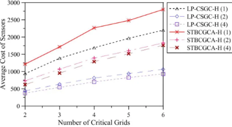
Fig. 10. Average costs of sensors deployed by STBCGCA-H and the average lower bounds of the optimal solutions to CRITICAL-SQUARE-GRID COVERAGE-H evaluated by LP-CSGC-H in sensor fields divided into10×10 grids of squares with lengthℓ and having 2 to 6 critical grids, where 𝑘 denotes
the number of the types of the sensors, and the types of sensors(𝑅𝑠, 𝑅𝑡, 𝑐𝑜𝑠𝑡)
are(√1
2ℓ, ℓ, 150) as 𝑘 = 1, (√12ℓ, ℓ, 150) and (√32ℓ, 3ℓ, 300) as 𝑘 = 2, and
(√1
2ℓ, ℓ, 150), (√12ℓ, 3ℓ, 200), (√32ℓ, ℓ, 250), and (√32ℓ, 3ℓ, 300) as 𝑘 = 4.
lower bound of the optimal solution to CRITICAL-SQUARE-GRID COVERAGE-H evaluated by LP-CSGC-H, which is reasonable.
VI. CONCLUSION
In this paper, we proposed an approximation algorithm, STBCGCA, for CRITICAL-SQUARE-GRID COVERAGE. STBCGCA constructs an auxiliary graph𝐺, uses Klein and
Ravi’s approximation algorithm [33] to establish a node-weighted Stenier tree 𝑆𝑇 in 𝐺, and selects a set of grid
points based on𝑆𝑇 so that sensors deployed on the selected
grid points form a connected wireless sensor network and fully cover all critical grids. To evaluate the performance of STBCGCA, we proposed another three algorithms, C-RNP, MSC-RNP, and MSC-MNWST, and investigated the numbers of sensors deployed by STBCGCA, C-RNP, MSC-RNP, and MSC-MNWST. C-RNP, MSC-RNP, and MSC-MNWST are all two-phase algorithms that deploy sensors to fully cover all critical grids in phase one and deploy sensors to establish the connectivity between sensors in phase two. Simulations show that STBCGCA deploys fewer sensors than C-RNP, MSC-RNP, and MSC-MNWST, in most cases. In addition, STBCGCA-H, an extension of STBCGCA, is proposed to form a connected wireless heterogenous sensor network.
In STBCGCA and STBCGCA-H, we employ disk sensing and communication models. To employ a non-disk sensing or communication model, such as the two-ray ground prop-agation model [40], the log-normal shadowing model [41], or the quasi unit disk graph model [42], the largest stable sensing and transmission ranges of a sensor are used as the sensing and transmission ranges of the sensor in STBCGCA and STBCGCA-H, respectively. For example, if STBCGCA or STBCGCA-H is used to deploy sensors adopted in [40] and [41], then the transmission range of the sensor is set to100 m and 20 m, respectively. This stems from their simulation results that show two sensors adopted in [40] and [41] can reach each other if their distance is not greater than 100 m and20 m, respectively. In the quasi unit disk graph model, given𝑝, 𝑟, and 𝑅, a sensor can detect an event with probability
1, 0, and 𝑝, if the distance between the sensor and the event is not greater than𝑟, greater than 𝑅, and within the interval
(𝑟, 𝑅], respectively. Therefore, if sensors employ the quasi unit disk graph model as the sensing model, then𝑟 is used as the
sensing range of the sensor as STBCGCA or STBCGCA-H is used to deploy the sensors.
REFERENCES
[1] P. Ray and P. Varshney, “Estimation of spatially distributed processes in wireless sensor networks with random packet loss," IEEE Trans.
Wireless Commun., vol. 8, no. 6, pp. 3162-3171, June 2009.
[2] K. K. Rachuri and C. Murthy, “Energy efficient and scalable search in dense wireless sensor networks," IEEE Trans. Comput., vol. 58, no. 6, pp. 812-826, June 2009.
[3] M. J. Tsai, H. Y. Yang, B. H. Liu, and W. Q. Huang, “Virtual-coordinate-based delivery-guaranteed routing protocol in wireless sensor networks,"
IEEE/ACM Trans. Networking, vol. 17, no. 4, pp. 1228-1241, Aug. 2009.
[4] A. O. Fapojuwo and A. Cano-Tinoco, “Energy consumption and mes-sage delay analysis of QoS enhanced base station controlled dynamic clustering protocol for wireless sensor networks," IEEE Trans. Wireless
Commun., vol. 8, no. 10, pp. 5366-5374, Oct. 2009.
[5] T. R. Park, K. J. Park, and M. J. Lee, “Design and analysis of asyn-chronous wakeup for wireless sensor networks," IEEE Trans. Wireless
Commun., vol. 8, no. 11, pp. 5530-5541, Nov. 2009.
[6] Z. Merhi, M. Elgamel, and M. Bayoumi, “A lightweight collaborative fault tolerant target localization system for wireless sensor networks,"
IEEE Trans. Mobile Comput., vol. 8, no. 12, pp. 1690-1704, Dec. 2009.
[7] V. Chvatal, “A combinatorial theorem in plane geometry," J.
Combina-torial Theory Ser. B, vol. 18, pp. 39-41, 1975.
[8] J. O’Rourke, Art Gallery Theorems and Algorithms. Oxford University Press, 1987.
[9] F. Hoffmann, M. Kaufmann, and K. Kriegel, “The art gallery theorem for polygons with holes," in Proc. IEEE FOCS, 1991.
[10] J. B. M. Melissen and P. C. Schuur, “Covering a rectangle with six and seven circles," Discrete Applied Math., vol. 99, no. 1, pp. 149-156, Feb. 2000.
[11] K. J. Nurmela, “Conjecturally optimal coverings of an equilateral triangle with up to 36 equal circles," Experimental Math., vol. 9, no. 2, pp. 241-250, 2000.
[12] K. J. Nurmela and P. R. J. Ostergard, “Covering a square with up to 30 equal circles," HUT-TCS-A62, Tech. Rep., 2000.
[13] S. Slijepcevic and M. Potkonjak, “Power efficient organization of wireless sensor networks," in Proc. IEEE ICC, 2001.
[14] H. Zhang and J. C. Hou, “Maintaining sensing coverage and connectivity in large sensor networks," J. Ad Hoc Sensor Wireless Netw., vol. 1, no. 1, pp. 89-123, Jan. 2005.
[15] Z. Zhou, S. Das, and H. Gupta, “Connected k-coverage problem in sensor networks," in Proc. ICCCN, 2004.
[16] C. F. Huang, Y. C. Tseng, and H. L. Wu, “Distributed protocols for ensuring both coverage and connectivity of a wireless sensor network,"
ACM Trans. Sensor Netw., vol. 3, no. 1, p. 5, Mar. 2007.
[17] C. Y. Chang, C. T. Chang, Y. C. Chen, and H. R. Chang, “Obstacle-resistant deployment algorithms for wireless sensor networks," IEEE
Trans. Veh. Technol., vol. 58, no. 6, pp. 2925-2941, July 2009.
[18] X. Han, X. Cao, E. L. Lloyd, and C. C. Shen, “Deploying directional sensor networks with guaranteed connectivity and coverage," in Proc.
IEEE SECON, 2008.
[19] K. Chakrabarty, S. S. Iyengar, H. Qi, and E. Cho, “Grid coverage for surveillance and target location in distributed sensor networks," IEEE
Trans. Comput., vol. 51, no. 12, pp. 1448-1453, Dec. 2002.
[20] X. Xu, S. Sahni, and N. Rao, “Minimum-cost sensor coverage of planar regions," in Proc. FUSION, 2008.
[21] F. Y. S. Lin and P. L. Chiu, “A simulated annealing algorithm for energy-efficient sensor network design," in Proc. ICST WiOpt, 2005. [22] X. Bai, S. Kumar, Z. Yun, D. Xuan, and T. H. Lai, “Deploying wireless
sensors to achieve both coverage and connectivity," in Proc. ACM
MobiHoc, 2006.
[23] A. Howard, M. J. Matari’c, and G. S. Sukhatme, “An incremental self-deployment algorithm for mobile sensor networks," Autonomous Robots, vol. 13, no. 2, pp. 113-126, Sep. 2002.
[24] N. Heo and P. K. Varshney, “An intelligent deployment and clustering algorithm for a distributed mobile sensor network," in Proc. IEEE SMC, 2003.
[25] A. Howard, M. J. Matari’c, and G. S. Sukhatme, “Mobile sensor network deployment using potential fields: a distributed, scalable solution to the area coverage problem," in Proc. DARS, 2002.
[26] Y. Zhou and K. Chakrabarty, “Sensor deployment and target localization in distributed sensor networks," ACM Trans. Embedded Comput. Syst., vol. 3, no. 1, pp. 61-91, Feb. 2004.
[27] M. Ma and Y. Yang, “Adaptive triangular deployment algorithm for unattended mobile sensor networks," IEEE Trans. Comput., vol. 56, no. 7, pp. 946-958, July 2007.
[28] Y. Zou and K. Chakrabarty, “A distributed coverage- and connectivity-centric technique for selecting active nodes in wireless sensor networks,"
IEEE Trans. Comput., vol. 54, no. 8, pp. 978-991, Aug. 2005.
[29] M. Cardei and D. Z. Du, “Improving wireless sensor network lifetime through power aware organization," ACM/Springer J. Wireless Netw., vol. 11, no. 3, pp. 333-340, May 2005.
[30] M. Cardei, M. T. Thai, Y. Li, and W. Wu, “Energy-efficient target coverage in wireless sensor networks," in Proc. IEEE INFOCOM, 2005. [31] W. C. Ke, B. H. Liu, and M. J. Tsai, “Constructing a wireless sensor network to fully cover critical grids by deploying minimum sensors on grid points is NP-complete," IEEE Trans. Comput., vol. 56, no. 5, pp. 710-715, May 2007.
[32] A. Segev, “The node-weighted Steiner tree problem," Netw., vol. 17, no. 1, pp. 1-17, 1987.
[33] P. N. Klein and R. Ravi, “A nearly best-possible approximation algo-rithm for node-weighted Steiner trees," J. Algoalgo-rithms, vol. 19, no. 1, pp. 104-115, July 1995.
[34] B. N. Clark, C. J. Colbourn, and D. S. Johnson, “Unit disk graphs,"
Discrete Math., vol. 86, no. 1-3, pp. 165-177, Dec. 1990.
[35] N. Heo and P. K. Varshney, “Energy-efficient deployment of intelligent mobile sensor networks," IEEE Trans. Syst., Man, Cybernetics-Part A:
Syst. Humans, vol. 35, no. 1, pp. 78-92, Jan. 2005.
[36] V. Chvatal, “A greedy heuristic for the set cover problem," Math.
Opererations Research, vol. 4, no. 3, pp. 233-235, Aug. 1979.
[37] R. M. Karp, Complexity of Computer Communications. Plenum, 1972. [38] E. L. Lloyd and G. Xue, “Relay node placement in wireless sensor networks," IEEE Trans. Comput., vol. 56, no. 1, pp. 134-138, Jan. 2007. [39] X. Cheng, D. Z. Du, L. Wang, and B. Xu, “Relay sensor placement in wireless sensor networks," ACM/Springer J. Wireless Netw., Jan. 2007. [40] A. A. Tamer Nadeem, “IEEE 802.11 fragmentation-aware
energy-efficient ad-hoc routing protocols," in Proc. IEEE MASS, 2004. [41] I. Stojmenovic, A. Nayak, J. Kuruvila, F. Ovalle-Martinez, and
E. Villanueva-Pena, “Physical layer impact on the design and perfor-mance of routing and broadcasting protocols in ad hoc and sensor networks," Comput. Commun., vol. 28, no. 10, pp. 1138-1151, June 2005.
[42] J. Chen, A. Jiang, I. A. Kanj, G. Xia, and F. Zhang, “Separability and topology control of quasi unit disk graphs," in Proc. IEEE INFOCOM, 2007.
Wei-Chieh Ke received the BSc and Ph.d. degrees
in computer science from National Tsing Hua Uni-versity in 2003 and 2011, respectively. His research interests include NP-hardness, mobile computing, distributed computing, mobile ad-hoc networks, and wireless sensor networks.
Bing-Hong Liu received the BSc and Ph.d. degrees
in computer science from National Tsing Hua Uni-versity in 2001 and 2008, respectively. In 2009, he joined the Department of Electronic Engineering at National Kaohsiung University of Applied Sciences, where he is currently an assistant professor. His research interests include mobile computing, dis-tributed computing, mobile ad hoc networks, and wireless sensor networks. He is a member of the IEEE.
Ming-Jer Tsai received the Ph.D. degree in
electri-cal engineering from the National Taiwan University in 1997. Since then, he has been with the Computer and Communication Laboratory, Industrial Technol-ogy Research Institute. He joined Department of Computer Science and Institute of Communications Engineering at National Tsing Hua University in 2003 and 2009, respectively, where he is currently an associate professor. His research interests include distributed systems and mobile computing. He is a member of the IEEE.
![[102-2] WNFA lab4 - A Tiny Wireless Sensor Network 2014/5/12 Chih-Hsien Ou](data:image/gif;base64,R0lGODlhAQABAIAAAP///wAAACH5BAEAAAAALAAAAAABAAEAAAICRAEAOw==)