Design and Implementation of an Adaptive Multilevel Scheduler in a Real-time Operating System

全文

(1)Design and Implementation of an Adaptive Multilevel Scheduler in a Real-time Operating System Liang-Teh Lee, Chia-Ying Tseng, Yu-Chieh Li, and Shieh-Jie Hsu Dept. of Computer Science and Engineering Tatung University, Taipei 104, Taiwan ROC ltlee@ ttu.edu.tw ABSTRACT The traditional researches on the task scheduling in real-time operating systems were setting the priority for providing service to soft tasks after that can promise meet deadline of hard tasks. Therefore, those scheduling schemes were trying to provide better average meet ratio for soft tasks. In this paper, an adaptive multi-level scheduler is proposed. The proposed architecture applies a tuner, called importance tuner, to evaluate the importance of each task, and to increase or decrease the weight of importance of the task. Then the task is assigned to the multiple EDF schedulers according to its importance weight. In addition to the multi-level EDF scheduler, we have also built a second level RM scheduler to schedule first level EDF schedulers as the normal tasks. Based on μC/OS-II, the proposed scheduling scheme has been implemented. The experimental results show that the proposed scheme can improve the system performance and fit for almost all real-time applications.. 1. INTRODUCTIONS A real-time system means that every task in the system must complete in time. There are two types of real-time systems: hard and soft real-time system [2].In hard real-time systems, tasks have to complete in time, but in soft real-time systems, tasks just need to complete as soon as possible but need not to finish before specific times. In safety critical environments it is necessary to verify a priority that a system design will meet the timing requirements of critical applications. Actually this requires the programmers to put some constrains on program structure. In such systems, it is customary to assume that the application consists of a set of tasks whose periods, execution times, and other resource requirements are known in advance. Under these suppositions, we can verify and solve a scheduling problem. If hard real-time systems have predictable behaviors and the necessary attributes of the tasks are known in advance, then the system can be analyzed with a scheduling test and we can develop a scheduling algorithm to meet the real-time requirement, i.e., deadline, of the system. In soft real-time systems, occasionally missing deadline is allowed. These systems are used in non-critical environments.. In the real world, there are systems running under an environment that consists of tasks with different types of deadline, hard deadline, soft deadline, and non real-time tasks, simultaneously. Those tasks with hard deadlines must be guaranteed to meet their deadlines, while tasks with soft deadline may be allowed to miss their deadlines occasionally, and the tasks of non real-time can be postponed. So most scheduling algorithms were just trying to provide better average meet ratio for soft tasks. But that have no considerate of the deadline of each task. The Adaptive Multilevel Scheduler we proposed can increase the average meet ratio for soft tasks, and it will be discussed more detailed in the section3. In the following, Section 2 discusses some background related to this paper. Section 3 introduces the architecture of the proposed adaptive multi-level scheduler. Section 4 describes the implementation details. Section 5 compares the performance of with other schedulers. Finally, Section 6 presents the conclusion.. 2. BACKGROUND A real-time operating system (RTOS) is developed for real-time applications and typically used for embedded applications on a special-purpose computer with a limited set of functions determined by the hardware design. Ideally, an RTOS provides a robust set of system services and a flexible task scheduling system without adversely affecting performance, requiring excessive memory, or overly imposing a code structure. More succinctly, an RTOS should be efficient and easily configurable while offering a feature-rich development environment. To achieve above conditions, the next generation real-time systems must be designed to be dynamic, predictable, and flexible [6]. Most RTOS kernel is priority based. Scheduler assigned unique priority to every task according to its importance. There are two kinds of scheduling algorithms: static scheduling algorithm and dynamic scheduling algorithm. Dynamic scheduling algorithm can change priorities at run time; on the contrary, static scheduling algorithm cannot. Typically, RTOS uses static scheduling algorithm, i.e., each task is assigned a fixed priority, and the task with highest priority is allocated to the processor [1]. The well-known examples of static scheduling algorithm is Rate-Monotonic (RM) algorithm [11] and the most popular dynamic scheduling algorithms are earliest-deadline-first (EDF), minimumlaxity-first (MLF) [8], and maximum-urgency-first. - 219 -.

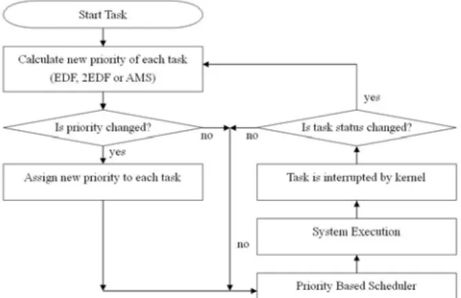
(2) (MUF) [10]. The Adaptive Multilevel Scheduler we proposed is mixed with static and dynamic scheduling algorithms, and it will be discussed more detailed in the next section. We implement the adaptive multi-level scheduler on μC/OS-II [2], a powerful but small RTOS kernel. And it is highly CPU independent and has been ported to numerous microprocessor platforms. Figure 1 shows the task states and functions provided by μC/OS-II. Each task typically is an infinite loop that can be in any one of five states: DORMANT, READY, RUNNING, WAITING (for an event) and ISR (interrupted), the DORMANT state corresponds to a task that resides in memory but has not been made available to the multitasking kernel. A task is READY when it can execute but its priority is less than the currently running task. A task is RUNNING when it has control of the CPU. A task is WAITING when it requires the occurrence of an event ,waiting for an I/O operation to complete, a shared resource to be available, a timing pulse to occur, time to expire, etc. Finally, a task is in the ISR state when an interrupt has occurred and the CPU is in the process of servicing the interrupt.. 3.1 RM/EDF Mixed Scheduler An RM/EDF mixed scheduler using μC/OS-II as the kernel and expanding the RM scheduler of μC/OS-II is implemented in this scheme. In order to simulate this scheme effectively, the tick time is set to 100ms, and execution time, deadline and period of tasks are set to the multiple of the tick time. A new priority of each task is assigned during each tick interrupt. The RM/EDF mixed scheduler can be achieved without modifying the kernel of μC/OS-II. The priority change mechanism is shown in Figure 2. Moreover, this mechanism is used in a multi-level scheduler called RM/EDF mixed schedulers that is shown in Figure 3. The RM/EDF Mixed scheduler is implemented. There are three scheduling policies in this scheme. In the first level, RM scheduler is dedicated to system task and EDF is dedicated to other tasks. In the second level scheduler, both of two first level schedulers, RM scheduler and EDF scheduler, are scheduled as normal tasks. RM Scheduler becomes to task A, and EDF scheduler becomes to task B in the second level scheduler.. Figure 1. Task States. 3. PROPOSED MULTI-LEVEL SCHEDULING. Figure 2. The Mechanism of Schedule Extension. The idea behind this model is based on the intuitive observation of the traditional scheduler system. A real-time operation system is running in the real environment that is not only containing single task form. The task is usually with different feature, different soft and hard real-time requirements, different executing time and deadlines, and different periods. Traditional researches usually were focused on achieving the best performance in using single scheduling architecture. It results in confusing of hard and soft real-time tasks, and the low average system performance. Moreover, an unpredictable error will occur easily when the system is overloaded. In this section, the proposed adaptive multi-level scheduler, based on previous analysis, will be introduced. We were bringing up several derivative architectures and apply different architectures according to the features of task set to achieve a better performance. RM and EDF scheduling schemes are used in the proposed architecture.. Figure 3. The RM/EDF Mixed Scheduler. 3.2 Double EDF Scheduler In the real-time operation system, a task with hard real-time requirement is usually means that more important to the system, i.e., the system will be damaged. - 220 -.

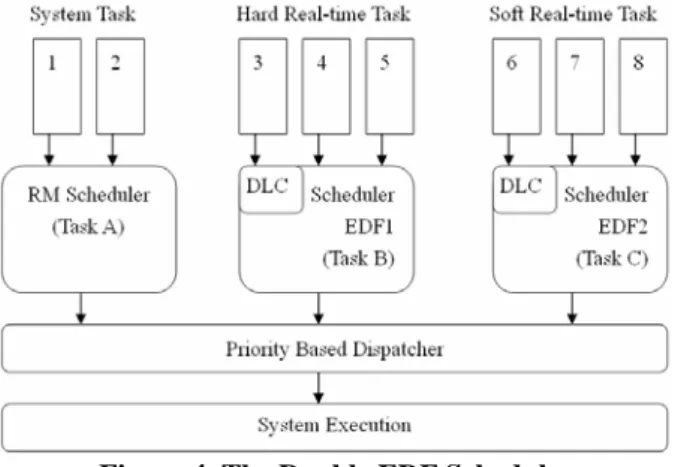
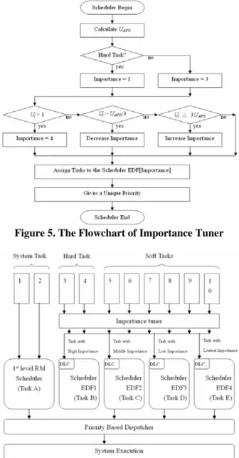
(3) when the task is fail or misses its deadline. The RM/EDF Mixed scheduler that we described in Section 3.1 could cause lethality error when hard and soft tasks are scheduled together. Therefore, based on the previous RM/EDF Mixed scheduler, an additional EDF scheduler is added to the RM/EDF Mixed architecture. New architecture is called double EDF. Totally there are two EDF schedulers that used to scheduling hard and soft real-time tasks individually. Figure 4 is the architecture of the scheduler. There are three scheduler, RM, EDF1, and EDF2, in the double scheduling scheme in the first level. The RM scheduler is dedicated to the system task, scheduler EDF1 is dedicated to hard real-time tasks and scheduler EDF2 is dedicated to soft real-time tasks. Execution of the three schedulers in the first level, including an RM scheduler and two EDF schedulers, can be scheduling as a normal task in the second level scheduler. In Figure 4, task A represents the first level RM Scheduler, task B represents scheduler EDF1 and task C represents scheduler EDF2. The second level RM scheduler is used to schedule task A, B and C. This module is based on a concept that the hard and soft tasks are scheduled individually. The utilization U of soft tasks is not relating to the meet ratio of hard tasks, because the priority of the hard task is always higher than priority of the soft task. Hard task could miss deadline only the utilization U of hard tasks is greater than 1.. Figure 4. The Double EDF Scheduler. 3.3 Adaptive Multi-Level Scheduler For two schedulers, RM/EDF mixed scheduler and double EDF scheduler, mentioned in the previous sections, there are still some problems. z Since RM/EDF mixed scheduler is scheduling hard and soft task in the same scheduler, hard tasks may miss their deadlines. z Double EDF scheduler is scheduling hard and soft tasks individually. Though it guarantees that each hard task will meet its deadline, the meet ratio of soft tasks will be decreased. For solving the above problems, an Adaptive Multi-Level Scheduler has been proposed to guarantee that hard task can meet its deadline and also can increase average meet ratio of soft tasks.. Based on the double EDF scheduler that we discussed in Section 3.2, Four EDF schedulers are used to schedule tasks. In addition, an importance tuner can use the execution time, deadline and period of each task to calculate the weight of importance for determining which EDF scheduler will be assigned for this task accordingly. The importance tuner will be described in the follows. Parameters used in the importance tuner are defined as follows: CT denotes Current Time, RT represents Remaining Execution Time, D is Deadline, and n is the number of tasks. RT and D of task i are denoted as RTi and Di respectively. The Urgency of Task i is defined as:. Ui =. RTi Di − CTi. (1). Average Urgency in the adaptive algorithm is defined as: n. U Avg =. ∑U i =1. n. i. (2). The steps for assigning importance and priority to each task are shown as follows. 1. Initialize the importance of each task. Importance of hard tasks is assigned to 1 and importance of soft tasks is assigned to 3. 2. Calculate the Average Urgency. 3. Increase the importance, subtract importance by one, when Ui ≧αUAvg or decrease the importance, add importance by one, when Ui <βUAvg. The values of α and β are set to 3 and 1/3 respectively. 4. Task is assigned the lowest importance, 4, if the Ui > 1. This means that the task is impossible to meet this deadline. 5. Tasks with importance 1, the highest importance, will be assigned to Scheduler EDF1. Tasks with importance 2 and 3 will be assigned to schedulers EDF2 and EDF3, respectively. Tasks with importance 4, the lowest importance, will be assigned to scheduler EDF4. 6. Assign a unique priority to every task in the EDF Schedulers individually. 7. Dispatch all tasks. The flowchart of importance tuner is shown in Figure 5. The added importance tuner was tuning the importance of hard and soft tasks in the permit range. Hard tasks can be forced to release CPU time when the situation is not very urgent, thus, soft tasks can use the limited system time to achieve their deadlines. Therefore the average meet ratio of soft tasks will be increased. The schedule level of the system is decided by the ratio of the urgency of single task to the average urgency. Therefore we named the scheme as Adaptive Multi-level scheduler.. - 221 -.

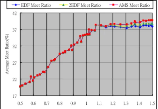
(4) Figure 6 is the architecture of the proposed adaptive multi-level scheduler.. z z z. Based on above-mentioned assumptions, two kinds of tasks will be created with different characteristics. Type1: Hard real-time tasks. Type2: Soft real-time tasks.. 5. PERFORMANCE EVALUATION Before the performance comparison, we have to define two formulas. Suppose there is a real-time operation system that consists of N tasks. The Average Meet Ratio and Average Miss Ratio can be defined as: AverageMeetRatio =. n. ⎛. i =0. ⎝. ∑ ⎜⎜ Meet. Figure 5. The Flowchart of Importance Tuner. Figure 6. The Adaptive Multi-level Scheduler. 4. IMPLEMENTATION For simulating a real-time operation system in real word, the real-time system is supposed to consists of hard tasks and soft tasks. Through setting soft/hard real-time requirement, execute time, deadline and period of each task, an actual real-time system can be simulated. z Kernel and Scheduler: Comparing to the execution time of a typical task, the execution times of the kernel and scheduler are relatively low. Therefore the execution time of the kernel and scheduler can be ignored. z Hard Tasks: The feature of hard tasks have regular period and cannot miss their deadlines. z Soft Tasks: This kind of tasks have regular appearance, they can miss their deadlines sporadically.. ×. ExecutionTimei Re leaseTimei. ⎞ ⎟⎟ ⎠. (3). ⎞ ⎟⎟ ⎠. (4). Tick × N n. AverageMissRatio =. i. ⎛. ∑ ⎜⎜ Miss i =0. ⎝. i. ×. ExecutionTimei Re leaseTimei. Tick × N. Since every task has individual execution time, therefore, comparing two tasks by their meet times is unfair. So Average Meet Ratio is calculated by multiplying meet times to the execution time to get the weighted value. Average Meet Ratio evaluates effective CPU time through calculating Meet times and Execution time. We can evaluate Average miss ratio is under similar concept. There are 50 task sets tested in our experiments. The utilization U of those task sets are between 0.5 and 1.5. The average meet ratio and average miss ratio are shown in Figure 7 and 8. All task sets scheduled by RM/EDF Mixed, double EDF and adaptive multi-level scheduler have same meet ratio and zero miss ratio when the utilization U is less than 1. But, our adaptive multi-level scheduler has the best performance when the utilization U is greater than 1. As above comparisons, the average meet/miss ratios changes depending on the utilization U of task sets, but the performance of Adaptive multi-level scheduler is always better than the other schedulers. In addition, we suppose that a real-time system consists of hard and soft tasks. Hard tasks are disallowed to miss deadline. Soft tasks are allowed to miss deadline, however, once a soft task misses its deadline, restart to execute the task is required. The results of 50 tested task sets is shown in Figures 9 and 10. The experimental results show that the proposed importance tuner is provided to guarantee the meet ratio of hard task when the utilization U is greater than 1. By this way, the system will be protected to avoid danger. Moreover, meet ratio of soft task can be improved to keep the system running smoothly. Finally, we have tried to find the best value of α and β. α and β depend upon execution time and period. Those values are inter-influenced. So it is difficult to find best α and β values. But the suggested range is provided during this paper. The better value of α is between 2.5 and 3.5 and the better value of β is between 0.2 and 0.5. In this suggested ranges, the performance of. - 222 -.

(5) adaptive multi-level scheduler is always better than traditional EDF, RM/EDF Mixed and double EDF schedulers. EDF Meet Ratio. 2EDF Meet Ratio. AMS Meet Ratio. 42. Average Meet Ratio(%). 37. 32. 27. 22. 17 0.5. 0.6. 0.7. 0.8. 0.9. 1. 1.1. 1.2. 1.3. 1.4. 1.5. Processor Utilization(U). Figure 7. Average Meet Ratio of All Schedulers EDF Misst Ratio. 2EDF Miss Ratio. AMS Miss Ratio. 12. Average Miss Ratio(%). 10 8. REFERENCES [1]. 4. 0 0.5. 0.6. 0.7. 0.8. 0.9. 1. 1.1. 1.2. 1.3. 1.4. 1.5. Processor Utilization(U). Figure 8. Average Miss Ratio of All Schedulers EDF Meet Ratio. 2EDF Meet Ratio. AMS Meet Ratio. 40 35 Average Meet Ratio(%). In this paper, an adaptive multi-level scheduler has been presented. This architecture combines the advantages of EDF and other Schedulers. The main concept of our scheduler schedules different kinds of tasks in an individual way. The developed importance tuner can assign task to the most suitable scheduler. The tasks are tuned to adapt to current system environment effectively. Therefore, hard tasks will be insured to meet deadlines and system is maintained to run safely. Also the system performance is improved. As the result of this research, the performance of proposed scheduler is better than the other schedulers. The system is supposed that all parameters of tasks are known a priori. Then the result can be calculated and predicted. So how to schedule the tasks when the execution time, period and deadline are unpredictable will be the key point of future researches.. 6. 2. 30 25 20 15 10 5 0 0.5. 0.6. 0.7. 0.8. 0.9. 1. 1.1. 1.2. 1.3. 1.4. 1.5. Processor Utilization(U). Figure 9. Average Meet Ratio of All Schedulers (Suppose Soft TaskLost Executed Progress when Miss Deadline) EDF Misst Ratio. 2EDF Miss Ratio. AMS Miss Ratio. 14 12 Average Miss Ratio(%). 6. CONCLUSIONS. 10 8 6 4 2 0 0.5. 0.6. 0.7. 0.8. 0.9. 1. 1.1. 1.2. 1.3. 1.4. 1.5. Processor Utilization(U). Figure 10. Average Miss Ratio of All Schedulers (Suppose Soft TaskLost Executed Progress when Miss Deadline). Bruno Dutertre and Victoria Stavridou, "Formal Analysis for Real-Time Scheduling," Proceedings of the 19th Digital Avionics Systems Conferences (DASC), vol. 1, pp. 1D4/1 -1D4/7, 2000. [2] Jean J. Labrosse, MicroC/OS-II, The Real-Time Kernel, R&D Books, 1999. [3] Jean J. Labrosse, Embedded Systems Building Blocks, R&D Books, 2000. [4] C. M. Krishna and Kang G. Shin, Real-Time Systems, McGraw-Hill, 1997. [5] J.E. Cooling, Software Design for Real-Time Systems, Chapman & Hall, 1991. [6] Krithi Ramamritham and John A. Stankovic, "Scheduling Algorithms and Operating Systems Support for Real-Time Systems," Proceedings of the IEEE, vol. 82, No. 1, pp. 55 –67, Jan. 1994. [7] John A. Stankovic, Marco Spuri, Marco Di Natale, and Giorgio C. Buttazzo, "Implications of Classical Scheduling Results for Real-Time Systems," IEEE Computer, vol. 28, No. 6, pp. 16 –25, June 1995. [8] Liu, C. L., and J. W. Layland, “Scheduling Algorithms for Multiprogramming in a Hard Real Time Environment,” Journal of the Association for Computing Machinery, vol.20, no.1, pp. 44-61, January 1973. [9] S. K. Baruah, L. E. Rosier, and R. R. Howell, "Algorithms and Complexity Concerning the Preemptive Scheduling of Periodic Real-Time Tasks on One Process," The Journal of Real-Time Systems, vol. 2, pp. 301-324, 1990. [10] David B. Stewart and Pradeep K Khosla, “Real-Time Scheduling of Dynamically Reconfigurable System,” Proceedings of the IEEE International Conference on Systems Engineering, pp. 139-142, August 1991. [11] Lehoczky, J., L. Sha, and Y. Ding, “The Rate Monotonic Scheduling Algorithm: Exact Characterization and Average Case Behavior,” Proceedings 10th IEEE Real-Time Systems Symposium, Santa Monica, CA, pp. 166-171, December 1989.. - 223 -.

(6)