A New Normal Walk Model for Cellular Networks

全文

(1)ICS’02. B10334. <<. Workshop on Computer Networks. >>. A New Normal Walk Model for Cellular Networks Chen-Chau Yang 1, *. Chiu-Ching Tuan 1, 2, 1. Department of Electronic Engineering. National Taiwan University of Science and Technology 43, Sec. 4, Keelung Rd, Taipei 106, Taiwan, R.O.C. 2. Department of Electronic Engineering. National Taipei University of Technology 1, Sec. 3, Chung-Hsiao E. Rd, Taipei 106, Taiwan, R.O.C. [email protected]. [email protected]. Tel. No: +886-2-27712171 Ext. 2200. Tel. No: +886-2-27333141 Ext. 7214. Fax. No: +886-2-27317120. Fax. No: +886-2-27333800. Abstract In most two-dimensional random walk models, the directions of a mobile station or subscribe moving out of a cell are assumed to be independent and identical distributed. The mobility patterns obtained from such a model may be less sufficient and less effective to measure the performance of cellular networks. This paper presents a new normal walk model to provide a more realistic and more versatile mobility patterns. This model mainly utilizes an equivalent drift angle with normal distribution to determine the next moving-out direction in a hexagonal cellular network. The experimental results demonstrate that if let the standard deviation of drift angles, σ, be 71° , a normal walk could almost behave as a random walk. With three different σ, 15° , 30° , and 60° , the results show that the errors between the analysis values and the simulation values are all within ±0.75%, even ±0.5% for most test cases. Our normal walk model can be effectively used for evaluating the performance of cellular networks, based on those more realistic and more objective mobility patterns. Key words: mobile station or subscriber, cellular networks, mobility patterns, random walk model, normal walk model.. *. Correspondence author: Prof. C.-C. Yang. 1 / 18.

(2) ICS’02. B10334. I. Introduction In cellular or personal communication services (PCS) networks, the networking performance is significantly affected by the way the network managing the mobile stations or subscribes (MS). Hence designing the networking strategies for: location updating (LU), paging, cell and location area layout, and radio resource arrangement, often need mobility models to evaluate the performance. That is, the mobility patterns play a critical role in measuring and analyzing the performance of cellular networks. Especially, if the walk model is less realistic or even unrealistic, the research results and conclusions would be less accurate or even invalid [3, 5, 11]. The two-dimensional (2-D) random mobility models are still extensively used in most existing analytic or simulation-based studies of cellular networks. The major applications utilizing those walk models include modeling microcell/macrocell PCS networks [1], modeling distance-based LU [1, 6, 7, 11] and movement-based LU [2, 11], modeling GPRS mobility management [1], pre-fetching/caching location-dependent data [9, 10], and tracking MS movements [12]. Next, we briefly state the mobility assumptions used by those authors. Akyildiz et al. [1] develop an analytical model for the new 2-D random walks based on [2], in which the moving probability for each direction is assumed to be uniform distributed. Tseng and Hung [8] also let the moving probability be uniform distributed in their analytical random walk model improved from [1]. The authors of [4, 6, 11] design a non-equal (i.e., non-uniform and also not normal distributed) moving probability used in their simulation-based random walk model. Especially, the design of the turning probabilities in [4] is completely based on the street layout. Tsai and Jan [7] utilize a rotation angle to determine the next moving direction, either going straight or turning back. The probability distribution for this angle is assumed to be normal, used in their analytical mobility model.. Tuan et al. [9, 10]. define a simulation-based model for normal walks in a mesh cellular network, in which an equivalent drift angle is used for deciding the moving-out direction, and the probability of this drift angle is also normal distributed, originated in [7]. As described above, in most random walk models, the directions of an MS moving outside a cell are assumed to be independent and identical distributed. The mobility patterns obtained from such a model may be less sufficient and less effective to investigate the performance of cellular networks. Even though some simulation-based mobility. 2 / 18.

(3) ICS’02. B10334. models use non-equal probabilities developed under specific considerations, we think such a simulation-based model still needs to be validated by a corresponding analytical model. The purpose of this paper is to present an analytical model for the new normal walks used in the hexagonal cellular networks. The mobility patterns based on this normal walk model could be more realistic and more versatile for examining the performance of cellular networks. We also expected that a normal walk based on this model could nearly behave as a random walk, if let the standard deviation of drift angles, σ, be 71° . That is, the movement behavior of this normal mobility model under above σ could simulate that of the random mobility model. On the other hand, with different σ, the errors between the analysis values and the simulation values would be consistently all within ±0.75%, even smaller for most test cases. The major method for our model is to develop an equivalent drift angle with normal distribution and to confine the limit of each moving-out direction according to the geometric shape of a hexagonal cell (see Fig. 1a). Then the drift angles could be utilized to determine the next moving-out direction when an MS handoffs or handovers within a hexagonal cellular network. We expect that utilizing this normal walk model to measure performance of those applications as described previously, like modeling LU and modeling location areas, would be more effective and more objective than utilizing a random walk model. The remainder of this paper is organized as follows. Section II illustrates the new normal walks for hexagonal cellular networks, and describes the extended cell type classification. Section III validates the normal walk model with the performance comparisons, based on the macro-based state diagram. Finally, section IV concludes some research results in this paper.. II. The Hexagonal Normal walks Most two-dimensional (2-D) random walk models supposed that an MS moves into anyone of neighboring cells with equal probability, i.e., with probability 1/6.. Hence, in the hexagonal random walk model, an MS is initially at. the center of cell, and then the MS moves out of the current cell randomly via one of six absolute directions separated by 60° . As a result, in next movement, which cell an MS will visit is independent of the current cell the MS resides. Such a movement trace with high mobility may occur occasionally but not frequently, if contrasted. 3 / 18.

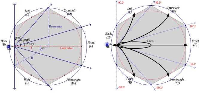
(4) ICS’02. B10334. with the daily movements of people.. A. The new normal walks. Based on the habit of people daily moving, we consider that the probability of an MS moving straight or front is often larger than that of moving via other directions, including U-turn, because most trips follow the shortest-path (namely, pseudo-linear routes) [7]. A drift angle, θ, is defined as a equivalent moving angle within one cell, by which the direction of an MS moving out of a cell could be determined. We further assume that the probability distribution of the equivalent drift angle, θ, approaches “normality”, with a zero mean (μ= 0° ) and a standard deviation, σ (unit in degree); namely, θ ~ N (0o , σ 2 ) .. Such a walk that uses a normal drift angle to decide the. next moving-out direction is called “normal walk model”. In our walk model, we assume that the inlets/outlets of a cell are located at the middles of six sides on a cell, which are marked ‘×’in Fig. 1a. Thus the rules of an MS moving outside a cell are as follows. First, an MS initially resides at some inlet/outlet of a cell. Next, the MS depends on a new normal drift angle to determine one of six r r relative moving-out directions, including moving straight or front ( F ), turning front-right ( Fr ), turning front-left. r r r r ( Fl ), turning right ( R ), turning left ( L ), and turning back ( B , i.e., U-turn). Last, the MS moves out of the cell via the selected direction as shown in Fig. 1b. For facilitate computing the probability of θ, the θ can be standardized into Z with the converting formula,. Z=. θ , where Z represents a standard normal random variable, i.e., Z ~ N (0, 1) . The pdf (probability density σ. function) of Z and the corresponding cdf (cumulative distribution function) of Z are as follows: ϕ ( z ) = and Φ ( z ) = ∫. z −∞. 1 2π. ⋅ e−z. 2. /2. ϕ ( y ) ⋅dy, where - ∞ < z < ∞ , respectively.. Hence the probabilities of an MS moving outside a cell via different directions could be obtained by (1) and (2). First, Fig. 1a shows that the limit of each moving-out direction is confined to two angles. The confined angles, angF, angFl, and angL could be easily computed with substituting the expression, r = R ×cos30° , where r and R denote the inner radius and outer radius, respectively, as shown in Fig. 1a. Formulas for calculating confined angles are as follows:. 4 / 18.

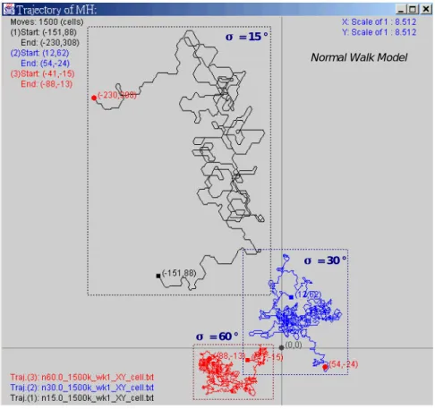
(5) ICS’02. B10334. 49.10. 90.00. Left (L). Left (L). Front-left (Fl) x. x. Front-left (Fl) x. x. 16.10. R (outer radius). angL. Back (B). x MS. Back (B). angFl angF r. 300. r (inner radius). x. Front (F). U-turn x. MS. Front (F). R -16.10. x. Right (R). x. x. -90.00. Fig. 1. Layout of a hexagonal cell.. x. Right (R). Front-right (Fr). Front-right (Fr) -49.10. (a) Limits of 6 moving directions. (b) 6 moving equivalent paths.. 0 .5 R ) ≅ 16.1o , 2r R angFl = tan −1 ( ) ≅ 49.1o , and r angF = tan −1 (. (1). angL = tan −1 (∞) = 90o. Then, with (1) and (2), the moving probabilities of a normal walk could be derived, e.g., let σ be 30° , thus. r r r r r r Pr[ F ,30o ] = 0.411, Pr[ Fr ,30o ] = Pr[ Fl ,30o ] = 0.244, Pr[ R,30o ] = Pr[ L,30o ] = 0.049, and Pr[ B,30o ] = 0.003. r angF Pr[ F , σ ] = 1 − 2 ⋅ Φ( ), σ r r angFl angF Pr[ Fl , σ ] = Φ ( ) − Φ( ) = Pr[ Fr , σ ], σ σ r r angL angFl Pr[ L, σ ] = Φ( ) − Φ( ) = Pr[ R, σ ], and σ σ r angL Pr[ B, σ ] = 2 ⋅ (1 − Φ( )). σ. (2). The all six moving-out probabilities as shown above are obviously not equal; however, the probability of turning right/front-right equals that of turning left/front-left, and also the summation of all probabilities must be one. Since the Φ(z) is function of the σ, changing the σ will lead to changing the moving-out probabilities. Naturally, the. r smaller the σ is, the larger the probability of moving front, Pr[ F , σ ] , is. Fig. 2 demonstrates that changing the σ could cause different styles of movement patterns or trajectories. It is clearly that the smaller the σ is, the broader the trajectory of an MS moving in a cellular network is.. 5 / 18.

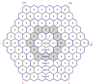
(6) ICS’02. B10334. σ = 15° Normal Walk Model. σ = 30°. σ = 60°. Fig. 2. Examples of the normal walk trajectories under σ = {15° , 30° , 60° }.. B. The extended cell type classification. Fig. 3 depicts a 6-layer hexagonal cellular cluster with (n2 + n)/2 cells (where n = 6). The cell at the center of the cluster is unique and called “central cell” or layer-0 cell. The cells that embraces the layer-(x – 1) are referred to as “inner cells” or layer-x cells, where 1 ≤ x < n – 1. Moreover, as x = n – 1, the cells at the most outer layer are called “border cells” or layer-(n – 1) cells. Especially, the cells embracing the border cells are termed as “boundary cells”, which are outside of the cluster. Except the central cell is only one in layer-0, each layer-x contains 6x cells, e.g., the layer-2 consists of 12 cells, which are shadowed at the second ring in Fig. 3. Following Akyildiz et al.’s cell type classification, a 6-layer cluster is partitioned into six equal pie-shape regions (pie-region) by three axes, L1-L3, separated by 60°as shown in Fig. 3. The equivalent cells will be assigned type ⟨x, y⟩, if cells are in layer-x and are at the relative y + 1st position on different pie-regions. This type classification significantly reduces the number of states of an n-layer random walk cluster from (3n2 + 3n – 5) to (n2 + n)/2, and efficiently speed up measuring the performance of analytical walk models.. 6 / 18.

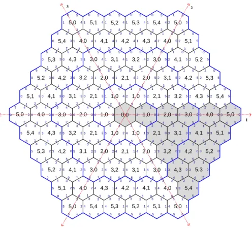
(7) ICS’02. B10334. L3. L2. 5. 5. 3. 4. 5 4 5. 3. 4. 3. 5 5. 2. 4 5 5. 3. 2 1. Layer-0 0. Layer-2 2. Layer-4 4. 5Layer-55. 5 4. 3 2. 1. 4. 3. 5 5. 4. L1. 5. 4 5. 4 4. 4 5. 4. 3 3. 4. 5. 3. 2. 2. 5. 3. 2. 3Layer-33 4. 5. 2. 5 4. 3. 1Layer-11 2. 4. 5 4. 3. 1 1. 3. 4. 3. 2. 3. 4. 4. 2. 2. 5. 5 4. 3. 4. 5 5. 5 4. 5. 5 5. 5. Fig. 3. An n-layer hexagonal cellular network, for n = 6.. Here, we extend the above classification method to be adapted for our normal walk model. In other words, afterclassifying all cells with type ⟨x, y⟩ (where 0 ≤ x < n and 0 ≤ y < x), we further add side indices, is (where 0 ≤ s < 6), to each of the typed cells. Afterwards, each side on a cell will be indexed as ⟨x, y, is⟩, where the order of is is from i0 to i5 in a counter-clockwise direction. This extended classification could facilitate modeling an n-layer cellular cluster for normal walks as shown in Fig. 4., and it will be described in detail later. The basic correlation between any both neighboring sides, ⟨x, y, is⟩ and ⟨x’, y’, it⟩, on the same pie-region is that s = mod6(t + 3) (where the modn denotes a modulus-n function), e.g., both ⟨4, 2, i0⟩ and ⟨5, 2, i3⟩ are neighboring sides. The other basic correlation between both ⟨x, y, ia⟩ and ⟨x, y, ib⟩ sides on the same cell is stated as below.. r r r r r r First, let Dir[k ] = {B, R, Fr , F , Fl , L} where 0 ≤ k ≤ 5, i.e., each member of Dir[k] represents one of six moving-out directions (see Fig. 1b). Next, suppose the path of an MS moving through a cell is from the ⟨x, y, ia⟩ side to the ⟨x, y, ib⟩ side (i.e., from the ia inlet to the ib outlet on the ⟨x, y⟩ cell) via the kth direction. Thus the value of ib could be derived from the expression, b = mod6(a + k), if ia and k are given. Here, we assume that the ib side, an MS will reach in next step via the kth direction, is function of the ia side, the MS resides at now; namely, the next side, ib, is independent of any cell sides that the MS visited previously. For example, if an MS moves from the ⟨4, 2, r i4⟩ side and towards the front-right ( Fr , k = 2), then the MS will reach the ⟨4, 2, i0⟩ side (or the neighboring ⟨5, 2,. i3⟩ cell) after one step.. 7 / 18.

(8) ICS’02. B10334. 3. 2. 0. 5,0. 1. 5. 4. 5,4 2 2 5. 1 5. 4. 5,2 2 5. 1 5. 4. 5,1. 0. 2 5. 1 5 0. 4. 5,0 2 4. 1 5. 4. 2 4. 1 3. 5,4. 5. 3. 3. 5,3 1 4. 0 5. 1. 5 4. 4 3. 5,2 1 4. 0 5. 3. 4,1. 2 5. 3. 1 4. 0 5. 3. 1. 2 4. 5. 5. 0. 1 4. 0 3. 2. 5 1 4. 0. 5. 0 3. 2. 0. 1 4. 5. 0. 1 4. 0. 5. 4 0. 0. 5. 1 0. 5. 4 2. 5,0 5. 1. 1. 1. 4. 5,4. 13. 0 3. 2. 5,1 5. 2. 0. 5. 4. 5,3. 0 3. 5 2. 4. 4,0. 1 4. 1. 1. 5,2. 0 3 5 2. 4. 4,3. 1 3. 0 3. 2. 5. 5,2. 2. 5. 4,1. 1 4. 0 3. 2. 5,3 5. 5. 5 2. 1. 5. 4. 5,1. 0 3. 5 2. 1. 5,0. 0 3. 5 2. 1. 4. 4,2. 0 3. 1. 4. 4,1. 0 3. 5 2. 1. 4. 3,0. 1 4. 1. 4. 3,2. 1 3. 0 3. 2. 3,1. 4,2. 1 4. 0 3. 2. 5,4. 0 3. 2. 5. 0 3 1 4. 2. 5 2. 5. 4 2. 3. 4,0. 0 3. 0. 5,4. 5 2. 4 2. 1. 4. 3,1. 0 3. 5 2. 4. 2,0. 1 4. 1. 0. 3. 3,0. 0 3. 5 2. 4. 2,1. 1 3. 0 3. 2. 2. 5. 4,3. 2 4. 1 3. 0. 5,0 0. 3. 5. 5. 3,2. 2 4. 1 3. 0. 4,0. 2 5. 3. 1,0. 2 4. 2,1. 2 4. 1 3. 0. 3,0. 2 5. 1 4. 0. 5,1. 1 4. 0. 3. 2,0. 2 5. 2. 1. 2,0. 0 3. 5 2. 4. 3. 1 3. 0. 1. 4 2. 3. 5 4 1. 3. 4,3. 5 2. 0. 5,3. 5 2 4 1. 0. 5. 4 1. 0. 3. 3,2. 5 2. 4 2. 3. 1,0. 3. 3. 1,0. 2 5. 1 4. 3. 3,1. 0 5. 2 4. 3. 0. 0,0. 3. 4 1. 0. 2,1. 5 2. 4 2. 3. 4. 1. 2,1. 2 5 1 4. 0. 4,2. 2 3. 3. 0. 3. 4,2. 5 2. 0. 5,2. 5 2. 4 1. 0. 3. 5 4 1. 0. 3. 3,1. 5 2. 4 1. 3. 1,0. 4 2 3. 2. 1,0. 3 0 2 4. 1. 3,2. 2 5. 1 2. 0. 4. 5. 4 1. 0. 2,0. 4 2. 3 1. 2. 1,0. 3 1. 2 5. 1. 2,0. 3 0. 2 4. 1. 4,3. 2 5. 1 4. 0. 4. 4. 5. 3. 3. 4,1. 5 2. 0. 5,1. 5 2 4 1. 0. 3,0. 4 2. 3 1. 2. 2,1. 4 1. 3 0. 2. 2,1. 3 0. 2 5. 1. 3,0. 3 0. 4. 5. 5. 0. 3. 5 4 1. 3. 4,0. 4 2. 3 1. 2. 3,2. 4 1. 3 0. 2. 2,0. 3 1. 2 5. 1. 3,1. 3 0. 2 5. 1. 4,0. 3 0. 4. 4. 5. 5. 0. 5,0. 4 2. 3 1. 2. 4,3. 4 1. 3 0. 2. 3,1. 4 1. 3 0. 2. 3,2. 3 0 2 5. 1. 4,1. 3 0. 4. 5. 5. 1. 5. 5,4. 4 1. 3 0. 2. 4,2. 4 1. 3 0. 2. 3,0. 0 1 3. 2 5 5. 4 1. 4,2. 3 0. 1 4. 5. 0. 5. 5,3. 4 1. 3 0. 2. 4,1. 4 1. 3 0. 2. 4,3. 3 3 0. 2 5. 1. 5 0. 4. 5,3. 0. 5. 0. 5. 5,2. 4 1. 3 0. 2. 4,0. 3 1. 0. 5. 5,1. 4 1. 3 0. 2 0. 0. 5. 1. 0. Fig. 4. The extended type classification with side indices for a 6-layer cellular cluster.. For classifying cells, Definition 1 indicates when cells on different pie-regions are equivalent and could be classified with the same cell types ⟨x, y⟩. Definition 1: Two cells, Ci and Cj, are considered as “equivalent”, if and only if, the multiset of side indices for Ci‘s neighboring sides equals that for Cj‘s neighboring sides, in corresponding order. The extended type classification for an n-layer normal walk cluster is described in Stage 1 and 2, based on the algorithm in [1]. Through the steps in Stage 1, all the equivalent cells on different pie-regions are assigned same types ⟨x, y⟩, where x and y denote that cells are at the y + 1st position in layer-x. Steps in Stage 1, required for assigning cell types, are shown as below. Step 1.1) For the central cell in layer-0, it is assigned type ⟨0, 0⟩. Step 1.2) In layer-x (where 1 ≤ x < n), identify the cells that are unmarked and are adjacent to ⟨x – 1, 0⟩ cells being labeled in layer-(x – 1), and then assign them with the type ⟨x, 0⟩. Thus the last six unmarked cells will be typed as ⟨n – 1, 0⟩ in this recursive step. Step 1.3) If the cells neighboring to ⟨x, y – 1⟩ cells in the same layer-x (where 2 ≤ x < n and 1 ≤ y < x) are still. 8 / 18.

(9) ICS’02. B10334. unmarked, then assign them with the type ⟨x, y⟩ recursively in the clockwise direction. Thus the last six marked cells are typed as ⟨n – 1, n – 2⟩ in this step. Next, Stage 2 further assigns the side indices (SI) for all cells, typed as ⟨x, y⟩ in Stage 1, through the following steps. For clarifying the expressions as below, the symbol i[k] is same as ik, and the value of ik is equal to k. Step 2.1) For the ⟨0, 0⟩ cell, its six sides are indexed as ⟨0, 0, i0⟩, because its all neighboring cells are of the same type ⟨1, 0⟩. Step 2.2) For ⟨x, 0⟩ cells (where 1 ≤ x < n), find the unmarked sides that are adjacent to the marked ⟨x – 1, 0, i0⟩ sides in layer-(x – 1), and then assign them with the index ⟨x, 0, i[mod6(i0 + 3)]⟩, i.e., ⟨x, 0, i3⟩. Then find sides that are unmarked on ⟨x, 0⟩ cells, and then sequentially index them as ⟨x, 0, i[mod6(i3 + s)]⟩ from s = 1 to s = 5 in the count-clockwise direction. Thus the multiset of SI on ⟨x, 0⟩ cell is {⟨ x, 0, i3⟩, ⟨ x, 0, i4⟩, ⟨ x, 0, i5⟩, ⟨ x, 0, i0⟩, ⟨ x, 0, i1⟩, ⟨ x, 0, i2⟩} in the order indexed. Step 2.3) For ⟨x, y⟩ cells (where 2 ≤ x < n and 1 ≤ y < x), find the unmarked sides that are neighboring to the marked ⟨x – 1, y – 1, i5⟩ sides in layer-(x – 1), and then index them as ⟨x, y, i[mod6(i5 + 3)]⟩, i.e., ⟨x, y, i2⟩. Then assign the unmarked sides on ⟨x, y⟩ cells with the index ⟨x, y, i[mod6(i2 + s)]⟩ from s = 1 to s = 5 in the count-clockwise direction. Hence the multiset of SI on this cell is {⟨ x, y, i2⟩, ⟨ x, y, i3⟩, ⟨ x, y, i4⟩, ⟨ x, y, i5⟩, ⟨ x, y, i0⟩, ⟨ x, y, i1⟩} in the order indexed. For an n-layer normal walk cluster, It is easy to examine that the extended classification algorithm possesses the following properties. 1) For the ⟨0, 0⟩ central cell, if n > 1, the ⟨0, 0⟩ cell’s neighboring sides are all same and indexed as ⟨1, 0, i3⟩. If n = 1, its neighboring sides are all outside the cluster and indexed as “Boundary ⟨0, 0, i0⟩”. 2) For a ⟨x, 0⟩ inner cell (where 1 ≤ x < n – 1), the multiset of SI for its neighboring sides is {⟨x + 1, 0, i3⟩, ⟨x + 1, x, i3⟩, ⟨x, x – 1, i4⟩, ⟨x – 1, 0, i0⟩, ⟨x, modx(1), i[mod6(1+ 1/x)]⟩, ⟨x + 1, 1, i2⟩}. For example, let x = 1, the multiset of SI for ⟨1, 0⟩ cell’s neighboring sides is {⟨2, 0, i3⟩, ⟨2, 1, i3⟩, ⟨1, 0, i4⟩, ⟨0, 0, i0⟩, ⟨1, 0, i2⟩, ⟨2, 1, i2⟩}. 3) For a ⟨x, y⟩ inner cell (where 2 ≤ x < n – 1 and 1 ≤ y < x), the multiset of SI of its neighboring sides is {⟨x + 1, y, i3⟩, ⟨x, y – 1, i4⟩, ⟨x – 1, y – 1, i5⟩, ⟨x – 1, modx-1(y), i[mod6(y/(x – 1))]⟩, ⟨x, modx(y + 1), i[mod6(1 + (y. 9 / 18.

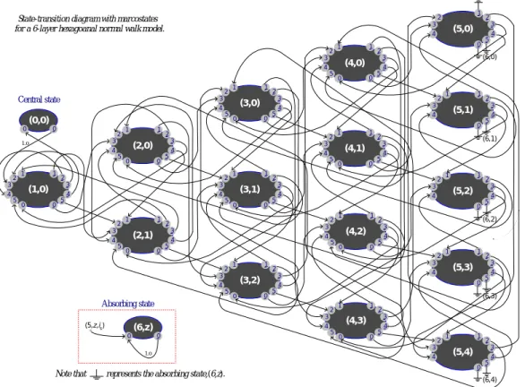
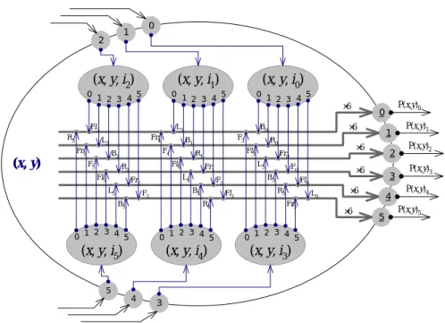
(10) ICS’02. B10334. + 1)/x)]⟩, ⟨x + 1, y + 1, i2⟩}. For instance, if x = 3 and y = x – 1, the multiset of SI for ⟨3, 2⟩ cell’s neighboring sides is {⟨4, 2, i3⟩, ⟨3, 1, i4⟩, ⟨2, 1, i5⟩, ⟨2, 0, i1⟩, ⟨3, 0, i2⟩, ⟨4, 3, i2⟩}. 4) For a ⟨n – 1, 0⟩ border cell (where n > 1), the multiset of SI for its neighboring sides is {⟨ n – 1, n – 2, i4⟩, ⟨n – 2, 0, i0⟩, ⟨n – 1, modn–1(1), i[mod6(1 + 1/(n – 1))]⟩, Boundary ⟨n – 1, 0, i0⟩, Boundary ⟨n – 1, 0, i0⟩, Boundary ⟨n – 1, 0, i0⟩}. For example, if n = 6, the multiset of SI for ⟨5, 0⟩ cell’s neighboring sides is {⟨5, 4, i4⟩, ⟨4, 0, i0⟩, ⟨5, 1, i1⟩, Boundary ⟨5, 0, i0⟩, Boundary ⟨5, 0, i0⟩, Boundary ⟨5, 0, i0⟩}. 5) For a ⟨n – 1, y⟩ border cell (where n > 2 and 1 ≤ y < n – 1), the multiset of SI for its neighboring sides is {⟨n – 1, y – 1, i4}⟩, ⟨n – 2, y – 1, i5⟩, ⟨n – 2, modn-2(y), i[mod6(y/(n – 2))]⟩, ⟨n – 1, mod n-1(y + 1), i[mod6(1 + (y + 1)/(n – 1))]⟩, Boundary ⟨n – 1, y, i0⟩, Boundary ⟨n – 1, y, i0⟩}.. For instance, let n = 6 and y = n – 2, the multiset of SI for ⟨5, 4⟩ cell’s neighboring sides is {⟨5, 3, i4⟩, ⟨4, 3, i5⟩, ⟨4, 0, i1⟩, ⟨5, 0, i2⟩, Boundary ⟨5, 4, i0⟩, Boundary ⟨5, 4, i0⟩}. The above properties and examples demonstrate that the extended type classification algorithm satisfies Definition 1. Also, the one-step probability of moving outside Ci equals that moving outside Cj if the starting and arriving sides, ⟨x, y, ia⟩ and ⟨x, y, ib⟩, for both movements are same.. III. Performance measuring and comparisons For a random walk model in [1], a typed cell corresponds to a state. However, for our normal walk model, a state is matched with an indexed side (inlet), based on the extended type classification. In the state-transition diagram, depicting all states, including absorbing ones, associated with probabilities may be too complicated for this model. Here, we develop a two-level state, macrostate and microstate, for clarifying the diagram. The new macro-based state transition diagram of a 6-layer cellular cluster for normal walks is shown in Fig. 5.. A. The macro-based state diagram. A macrostate (x, y) is an abstract state, and it just denotes that an MS resides one of the ⟨x, y⟩ cells through some side (inlet). Such a macrostate, excluding the central state (0, 0) and absorbing states (6, z), could be further split. 10 / 18.

(11) ICS’02. B10334. 3. 3 5 2. 5. (0,0) 2 3. 1.0. 5 1. 1. 3 5. 0. 0. 2 3. 4. 4. 5. 3. 4. 4 5 1. 5. 0. 0. (6,1). 5 2. 4. 4. 5. 5. 0. 0. 0. 5 1. 1. 3. 3 4. (6,3). Absorbing state. 2. 1. 1. 3. 2 3. (4,3). 4 5. 0. 0. 4 0. 5 2 3. 1.0. 5. 0. 4 5. (6,z). 2. (5,3). 4. 3 0. 4. (6,2). 2. (3,2). 4. 3 5. 3 4 2. 1. 2. (5,2). 2. (4,2) 5. 5. 1. 1. 4. 1. 1. 1. 0 2. 3. 0. 0. 0. 3. 2. (5,z,is). 4 5. 4. 3. 3 4 0. 0. 3. 3. 3. 2. (2,1). 4. 2. (5,1). 2. 2. (3,1). 5 1. 1. 1. 1. 1. (4,1) 5. 3. 2. 1. 1. 4. 3. 2. 3. 5. 2. 2. (1,0). 4. 0. 0. 2 3. 4. 0. (2,0). 4. 2. 1. 1. 3 0. 0. (6,0). 4 5. 2. (3,0). 4 0. 1. 1. 3. 4 0. 3 0. 0. 3 5. 2. (4,0). 4. Central state. 1. 1. 2. (5,0). 4 2. 0. 1. 2. State-transition diagram with marcostates for a 6-layer hexagoanal normal walk model.. 4. 1. 1. 2 3. (5,4). 4 5. 0. Note that. represents the absorbing state,(6,z).. (6,4). Fig. 5. The macro-based state-transition diagram for a 6-layer cellular cluster.. into at most 6 microstates (x, y, is), where 0 ≤ s ≤ 5, as shown in Fig. 6. A microstate (x, y, is) is a physical state, and it represents that an MS visits the ⟨x, y⟩ cell through the ⟨x, y, is⟩ side, i.e., the is inlet on the ⟨x, y⟩ cell. A microstate (n, z, i0) is absorbing one; also, it means that an MS moves out of the n-layer cluster through one of the ⟨n – 1, z, is⟩ sides. The actual number of microstates, mx,y, within one (x, y) macrostate equals the number of unique indexed sides (inlet) through which an MS can move into the ⟨x, y⟩ cell, e.g., m0,0 = 1, m2,1 = 6, and m5,2 = 4 (see Fig. 5). Since an n −1 x −1. indexed side matches to a microstate, the total number of microstates, S(n), is equal to. ∑ ∑ m x, y + n , i.e.,. x =1 y = 0. S (n) = (3n − 1)(n − 1) . Table 1 lists the number of microstates for different typed cells. For example, in a 6-layer cellular cluster, the S(n) is 85; in contrast, the number of macrostates, SM(n), is only 21, because SM(n) = (n2 + n)/2. Supposed that Probx,y[k] represents the probability of an MS moving out of a ⟨x, y⟩ cell from the is inlet to the it. r r r r r r outlet via the kth moving direction, belongs to Dir[k ] = {B, R, Fr , F , Fl , L} . For a (x, y) macrostate, Probx,y[k] naturally corresponds to the one-step transition probability that the system shifts outside the (x, y) macrostate from the is microstate via tth outlet, and Probx,y[k] = {Bs, Rs, Frs, Fs, Fls, Rs} where 0 ≤ s, t, k ≤ 5 (see Fig. 6). Thus if the. 11 / 18.

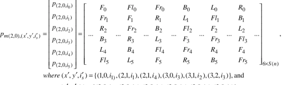
(12) ICS’02. B10334. 0. 1. 2. (x, y, i ). (x, y, i ). 2 0 1 5 2 3 4 Fl2 R5. 0 0 1 5 2 3 4. Fr5. L4. Fr2 L5. B3. F1 B4. F2 B5. F0. ×6 L0. Fr3. 2 3 4 0 1 5. 2 3 4 0 1 5. 2 3 4 0 1 5. (x, y, i5). (x, y, i4). (x, y, i3). P(x,y)3. 3. ×6 ×6. P(x,y)2. 2. Fl0 R3. Fl1 R4. P(x,y)1. 1. ×6. Fr0 L3. Fr1. P(x,y)0. 0. ×6 R0. Fl3. R1 Fl4. R2 Fl5. F3. B1 F4. B2 F5. ×6. B0. L1 Fr4. L2. (x, y). (x, y, i ). 1 0 1 5 2 3 4. P(x,y)4. 4 5. P(x,y)5. 5 4. 3. One Marcostate (x,y) contains 6 Microstates (x,y,is).. Fig. 6. Example of a macrostate comprising 6 microstates.. is (inlet) and it (outlet) are known, then the Probx,y[k] can be decided by the expression, k = mod6(t – s + 6), bywhich all one-step probabilities for any one macrostate, Pm(x, y), could be obtained. For instance, pm(2, 0),(x’, y’, is’) is for a ⟨2, 0⟩ cell as shown in Fig. 7, in which the ⟨x’, y’, is’⟩ sides are neighboring to the ⟨x, y, it⟩ sides. Table 1. The number of microstates/macrostates for a ⟨x, y⟩ cell. Cell types:. (a) Microstates, mx,y. (b) Macrostates. (a) ×(b). Central cell, ⟨0, 0⟩. ×1. 1. 1. Inner cells, ⟨x, y⟩. ×6. (n – 1)(n – 2)/2. 3(n – 1)(n – 2). Border cells, ⟨n – 1, z⟩. × 4 or × 3 (for z = 0) (n – 1). 4(n – 1) – 1. Boundary cells, ⟨n, z⟩. ×1. (n – 1). (n – 1). Total of microstates: S(n) = (3n – 1)(n – 1).. If let p( x, y,is ),( x′, y′,is′ ) be the probability that an MS moves from ⟨x, y, is⟩ side to ⟨x', y', is'⟩ side after one step, then P = [ p( x, y,is ),( x′, y′,is′ ) ] is the one-step transition probability matrix of the n-layer cluster for normal walks. Since the system has S(n) microstates, the size of matrix P is S(n) ×S(n). However, in matrix P, only n elements are constant, p(0,0,i0 ),(1,0,i3 ) = 1.0 and p( n, z ,i0 ),( n, z ,i0 ) = 1.0 , and the remainders are function of σ.. 12 / 18.

(13) ICS’02. B10334.  p( 2,0,i0 )  R0 L0 B0 Fr0 Fl0 F0       p( 2,0,i1 )   B Fl L R F Fr 1 1 1 1 1 1      L2 F2 Fl2 B2 Fr2 R2  p( 2,0,i2 )   ... ... ... ... ... ... , p m ( 2,0),( x′, y ′,is′ ) =  =  ...  Fl3 Fr3 F3 L3 R3 B3 p   ( 2,0,i3 )    F4 R4 Fr4 Fl 4 B4 L4  p( 2,0,i )    4    Fr5 B5 R5 F5 L5 Fl5  6×S ( n )  p( 2,0,i5 )   where ( x ′, y ′, is′ ) = {(1,0, i1) , (2,1, i1 ), (2,1, i4 ), (3,0, i3 ), (3,1, i2 ), (3,2, i3 )}, and ( x′, y ′, it ) = {( 2,0, i3) , (2,0, i4 ), (2,0, i2 ), (2,0, i0 ), (2,0, i5 ), ( 2,0, i1 )}.. Fig. 7. One-step transition probabilities only for one macrostate, e.g., pm(2, 0),(x’, y’, is’). The order of members listed in each rows and columns of matrix P corresponds to that of microstates listed by the following algorithm. 1. First, list the central state, i.e., (0, 0, i0). 2. Next, list all inner microstate, (x, y, is), as follows: for x = 1 to (n – 2) do for y = 0 to (x – 1) do for s = 0 to 5 do list (x, y, is). 3. Then, list the border ones: for y = 0 to (x – 1) do for s = 1 to 4 do list (n – 1, y, is), if existed. 4. Last, list the absorbing states, (n, y, i0): for y = 0 to (n – 2) do list (n, y, i0). Furthermore, for k = 1, (3) defines P ( k ) = [ pk ,( x, y,is ),( x′, y′,is′ ) ] as the probability that an MH moves from ⟨x, y, is⟩ side to ⟨x', y', is'⟩ side after k steps.. for k = 1  P, P (k ) =   P × P ( k −1) , for k > 1. (3). Thus pk ,( x, y,is ),( n, j ,i0 ) in (4) denotes the probability that an MH initially resides at a ⟨x, y, is⟩ side, and then moves outside a n-layer cluster through the ⟨n –1, j, it⟩ side. Later, we will evaluate the performances of a 6-layer cellular cluster for normal walks by using pk ,( x, y,is ),(6, j ,i0 ) .. for k = 1  P( x, y,is ),( n, j ,i0 ) ,  pk ,( x, y ,is ),( n, j ,i0 ) =  ( k ) ( k −1)  P( x, y,is ),( n, j ,i0 ) − P( x, y,is ),( n, j ,i0 ) , for k > 1. 13 / 18. (4).

(14) ICS’02. B10334. B. The performance analysis and comparisons. For validating the analytical normal walk model, we define two evaluation factors, S x, y. and T 5, z , based. on the equations Akyildiz et al.’s propose in [1]. First, S x, y represents the expected number of steps that an MH initially resides at a specified ⟨x, y⟩ cell, and then the MS leaves out of a 6-layer cluster through anyone of ⟨5, j⟩ border cells (where 0 ≤ j < 5).. ~ In contrast to S x, y , define S x, y in (5b) as the simulation values with M = 1,500,000 experimental trials, which are used to validate the analysis ones, S x, y , with 200 truncated terms to approach the infinite summation.. S. x, y. =. ∞. 4. 5. ∑ ∑ ∑ k ⋅ pk ,( x, y,is ),(6, j ,i0 ) ⋅. k =1 j =0 s =0. 1 . m x, y. ~ 1 M ~ S x, y = ⋅ ∑ s( x, y ) (i ) . M i =1. Next, let T 5, z. (5a). (5b). represent the other expected number of steps that an MH initially resides at anyone of ⟨x, y⟩ cells. (where 0 ≤ x < 5 and 0 ≤ y < x – 1) and then leaves the 6-layer cluster through a specified ⟨5, z⟩ cell. Be similar to. ~ (5a) and (5b), we define and calculate the simulation values, T 5, z , in (6b) to validate the analysis values, T 5, z . In (5a) and (6a), the 1/mx,y acts as a weight factor, where the mx,y is defined as previously.. T 5, z =. ∞. 5. ∑ ∑. k =1 x = 0. x −1. 5. ∑ ∑ k ⋅ pk ,( x, y ,is ),(6, z ,i0 ) ⋅. y =0 s =0. ~ 1 M ~ T 5, z = ⋅ ∑ t(5, z ) (i ) . M i =1. 1 . m x, y. (6a). (6a). In (3), the computing complexity required for obtaining P (k ) is generally at the order of O(S(n)3), where S(n) is the size of rows or columns. Since one hexagonal cell can neighbor at most six cells (outlets), each of rows in matrix P also contains no more than six non-zero elements. Obviously, matrix P is a spare matrix. Thus the order of computing P (k ) can be effectively reduced from O(S(n)3) to O(S(n)2) by utilizing this spare feature in our algorithms.. 14 / 18.

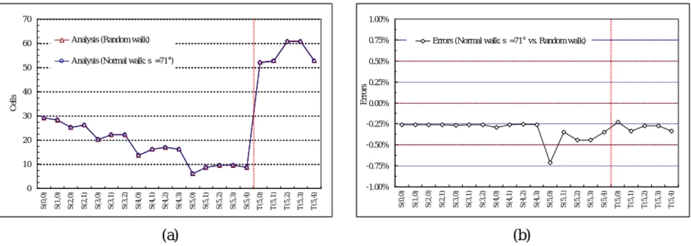
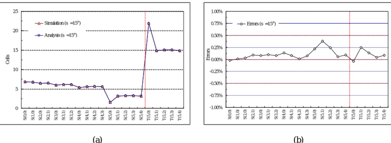
(15) ICS’02. B10334. Here, we define some notation to facilitate comparing performance, based on the above formulas. l. S n , Tn : Sets of analysis values, S x, y and T 5, z , respectively, under normal walk model.. l. ~ ~ ~ ~ S n , Tn : Sets of simulation values, S x, y and T 5, z , under normal walk model.. l. Sˆn , Tˆn : Sets of analysis values, S. x, y. and T 5, z , under normal walk model, but its moving probability is. forced with uniform distribution. l. S r , Tr : Sets of analysis values, L x , y and K 5, z , under random walk model [1], as the basis of. performance comparisons. First, we contrast the mobility behavior of an analytical normal walk under σ = 71°with that of an analytical random walk. The experimental results indicate that the performance curves of S n / Tn and S r / Tr are almost identical as shown in Fig. 8a. Hence, for comparing performance more clearly, Fig. 8b further illustrates the discrepancy between them for all test cases. The errors between both are within ±0.75%, and even only ±0.3% between Tn and Tr , as shown in Fig. 8b. Since the errors are small and within ±0.75%, we conclude that the mobility of normal walk under σ = 71°could nertly behave like that of the 2-D random walk. ~ ~ Next, we compare S n / Tn (analysis values) with S n / Tn (simulation values) to validate this normal walk model ~ ~ under three typical σ, 60° , 30° , and 15° . We observe that the performance curves of S n / Tn and S n / Tn are. almost overlapped and identical as shown in Fig. 9a, 10a, and 11a, respectively. On the other hand, Fig. 9b, 10b, and 11b illustrate that all errors between them are consistently within ±0.5%, even ±0.25% for most test cases. Also, we find that if let an MS initially reside at a specified ⟨x, y⟩ cell, then the movements required for the MS moving outside an n-layer cluster obviously decrease as the σ decreases, e.g., S(0, 0) = 23.7→10.9→6.8 (unit in steps) under σ = 60° →30° →15° , as expected. Last, let this normal walk model be with equal moving-out probability for each direction; that is, let it completely behave as a random walk model. We observe the errors between Sˆn / Tˆn and S r / Tr are really 0% (see Fig. 12). Accordingly, we think that the correctness of this analytic model and formulas as defined above could be demonstrated by this result indirectly.. 15 / 18.

(16) 0. -1.00%. (a). Fig. 10. Comparison on S/T (Analysis vs. Simulation, σ= 30° .) (a) Values of S/T.. 16 / 18 Errors (s =30°). 0.25%. -0.25% 0.00%. 10. -0.50%. -0.75% T(5,2). T(5,1). T(5,0). S(5,4). S(5,3). S(5,2). S(5,1). S(5,0). S(4,3). S(4,2). S(4,1). T(5,4). 1.00%. T(5,4). (b) Errors of S/T.. T(5,3). (b). T(5,3). T(5,2). T(5,1). T(5,0). S(5,4). 5. S(5,3). 0.50%. (a) Values of S/T.. S(5,2). 20. S(5,1). Fig. 9. Comparison on S/T (Analysis vs. Simulation, σ= 60° .) (a) Values of S/T.. S(5,0). 0.75%. Analysis (s =30°). S(4,3). (a). S(4,2). 25 Simulation (s =30°) S(4,0). (a). S(4,1). 30. S(4,0). -1.00% S(3,2). 10. S(3,2). 0.50%. S(3,1). Analysis (s =60°). S(3,1). 40. S(3,0). Fig. 8. Comparison on S/T (Normal walk, σ= 71°vs. Random walk.). S(3,0). 0.75%. S(2,1). 50 Simulation (s =60°). S(2,1). 60. S(2,0). (b). (b) Errors of S/T.. T(5,4). T(5,3). T(5,2). T(5,1). T(5,0). S(5,4). S(5,3). S(5,2). S(5,1). S(5,0). S(4,3). S(4,2). S(4,1). S(4,0). S(3,2). S(3,1). S(3,0). S(2,1). S(2,0). S(1,0). 20. S(2,0). Errors. 40. S(0,0). T(5,4). T(5,3). T(5,2). T(5,1). T(5,0). S(5,4). S(5,3). S(5,2). S(5,1). S(5,0). S(4,3). S(4,2). S(4,1). S(4,0). S(3,2). S(3,1). S(3,0). 0.50%. S(1,0). -1.00%. S(2,1). 0.75%. Analysis (Normal walk: s =71°). S(0,0). 30 Errors. 0 S(2,0). Analysis (Random walk). S(1,0). 15 Errors. T(5,4). T(5,3). T(5,2). T(5,1). T(5,0). S(5,4). S(5,3). S(5,2). S(5,1). S(5,0). S(4,3). S(4,2). S(4,1). S(4,0). S(3,2). S(3,1). S(3,0). S(2,1). -0.75%. S(1,0). 70. S(0,0). T(5,4). T(5,3). T(5,2). T(5,1). T(5,0). S(5,4). S(5,3). S(5,2). S(5,1). S(5,0). S(4,3). S(4,2). S(4,1). S(4,0). S(3,2). S(3,1). S(3,0). S(2,1). 10. S(0,0). Cells 50. S(2,0). S(1,0). S(0,0). Cells 60. S(2,0). S(1,0). 0. S(0,0). Cells. ICS’02 B10334. 1.00%. Errors (Normal walk: s =71° vs. Random walk). 0.25%. 30 0.00%. -0.25%. -0.50%. (b) (b) Errors of S/T.. 1.00%. Errors (s =60°). 0.25%. -0.25% 0.00%. 20 -0.50%. -0.75%.

(17) ICS’02. B10334. 25. 1.00%. Simulation (s =15°). 0.75%. Analysis (s =15°). 0.50%. Errors (s =15°). 20. Cells. Errors. 15. 10. 0.25% 0.00%. -0.25% -0.50%. 5. (a). T(5,4). T(5,3). T(5,2). T(5,1). S(5,4). T(5,0). S(5,3). S(5,2). S(5,1). (b). Fig. 11. Comparison on S/T (Analysis vs. Simulation, σ= 15° .) (a) Values of S/T.. 70. (b) Errors of S/T.. 1.00%. 60. Analysis (Random walk). 0.75%. Analysis (Normal walk: Prob.=1/6). 0.50%. Errors. 50. Cells. S(5,0). S(4,3). S(4,2). S(4,1). S(4,0). S(3,2). S(3,1). S(3,0). S(2,1). S(1,0). S(0,0). T(5,4). T(5,3). T(5,2). T(5,1). S(5,4). T(5,0). S(5,3). S(5,2). S(5,1). S(5,0). S(4,3). S(4,2). S(4,1). S(4,0). S(3,2). S(3,1). S(3,0). S(2,1). S(2,0). S(1,0). -1.00% S(0,0). 0. S(2,0). -0.75%. 40. Errors (Normal walk: Prob.=1/6 vs. Random walk). 0.25% 0.00%. 30 -0.25%. 20. (a). T(5,4). T(5,3). T(5,2). T(5,1). T(5,0). S(5,4). S(5,3). S(5,2). S(5,1). S(5,0). S(4,3). S(4,2). S(4,1). S(4,0). S(3,2). S(3,1). S(3,0). S(2,1). S(2,0). S(1,0). T(5,4). T(5,3). T(5,2). T(5,1). T(5,0). S(5,4). S(5,3). S(5,2). S(5,1). S(5,0). S(4,3). S(4,2). S(4,1). S(4,0). S(3,2). S(3,1). S(3,0). S(2,1). S(2,0). S(1,0). -1.00% S(0,0). -0.75%. 0. S(0,0). -0.50%. 10. (b). Fig. 12. Comparison on S/T (Normal walk, prob. = 1/6 vs. Random walk). (a) Values of S/T.. (b) Errors of S/T.. IV. Conclusions In cellular or PCS networks, the mobility patterns play a critical role in measuring and analyzing the performance of networks. Especially, if the mobility model, including random walks, is unrealistic, the research conclusions will be invalid. This paper presents a new analytical normal walk model to provide a more realistic and more versatile mobility patterns for measuring performance of networks. We conduct some experiments to demonstrate this normal walk model. The experimental results verify that when the standard deviation of drift angles, σ, is 71° , a normal walk could almost behave as a random walk, based on the performance curves of both are almost identical. Moreover, with different σ, 15° , 30° , and 60° , the results also indicate that the errors between the analysis values and the simulation values are all within ±0.75%, even ± 0.5% for most test cases. We think the normal walk model can be effectively used for examining the performance of 17 / 18.

(18) ICS’02. B10334. cellular networks, based on those more realistic and more objective mobility patterns. We need to apply this analytical normal walks in different applications, e.g., modeling microcell/macrocell PCS networks, modeling location update/paging, pre-fetching/caching location-dependent data, and tracking MS movements in our future works. Thus we can further investigate and improve this analytical model to be used more effectively in the study of cellular or PCS networks.. References [1] I. F. Akyildiz, Y.-B. Lin, W.-R. Lai, and R.-J. Chen, “A new random walk model for PCS networks,” IEEE J. Select. Areas Commun., vol. 18, No. 7, pp. 1254-1260, Jul. 2000. [2] I. F. Akyildiz, J. S. M. Ho, and Y.-B. Lin, “Movement-based location update and selective paging for PCS networks,” IEEE/ACM Trans. Networking, vol. 4, No. 4, pp. 629-638, Aug. 1996. [3] C. Bettstetter, “Mobility modeling in wireless networks: Categorization, smooth movement, and border effects,” ACM Mobile Comp. Commu. Review, vol. 5, No. 3, pp. 55-67, Jul. 2001. [4] K.-T. Chen, S.-L. Su, and R.-F. Chang, “Design and analysis of dynamic mobility tracking in wireless personal communication networks,” IEEE Trans. Veh. Technol., vol. 51, No. 3, pp. 486-497, May. 2002. [5] Y.-B. Lin and I. Chlamtac, “Wireless and mobile network architectures,” John Wiley & Sons, Inc., USA, 2001. [6] H.-W. Hwang, M.-F Chang, and C.-C. Tseng, “A direction-based location updates scheme with a line-paging strategy for PCS networks,” IEEE Commun. Lett., vol. 4, No. 5, pp. 149-151, May 2000. [7] I.-F. Tsai and R.-H. Jan, “The lookahead strategy for distance-based location tracking in wireless cellular networks,” ACM Mobile Comp. Commu. Review, vol. 3, No. 4, pp. 27-38, Oct. 1999. [8] Y.-C. Tseng and W.-N. Hung, “An improved cell type classification for random walk modeling in cellular networks,” IEEE Commun. Lett., vol. 5, No. 8, pp. 337-339, Aug. 2001. [9] C.-C. Tuan and C.-C. Yang, “Path-based data prefetch for mobile location-dependent information systems,” Proc. 8th Mobile Comp. Workshop, pp. 66-73, Taiwan, Mar. 2002. [10] C.-C. Tuan and C.-C. Yang, “Multi-version location-dependent data for path-based data prefetch mechanism,” Proc. NCS’01, Comp. Mobile Commu. Workshop, pp. E435-E445, Taiwan, Dec. 2001. [11] C.-H. Wu, “Unified analysis for location updates and probabilistic paging of PCS networks based on a 2D Markov walk model,” Proc. 8th Mobile Comp. Workshop, pp. 89-96, Taiwan, Mar. 2002. [12] M. M. Zonoozi and P. Dassanayake, “User mobility modeling and characterization of mobility patterns,” IEEE J. Select. Areas Commun., vol. 15, No. 7, pp. 1239-1252, Sep. 1997.. 18 / 18.

(19)