An Alternative Formulation for the Pricing of Stock Index Futures: Theoretical and Empirical Perspectives

全文

(1)International Journal of Business and Economics, 2007, Vol. 6, No. 2, 121-134. An Alternative Formulation for the Pricing of Stock Index Futures: Theoretical and Empirical Perspectives Chou-Wen Wang Department of Risk Management & Insurance, National Kaohsiung First University of Science & Technology, Taiwan Ting-Yi Wu* National Kaohsiung First University of Science & Technology, Taiwan and Department of Business Administration, Kao Yuan University, Taiwan. Abstract Assuming that a futures price is a function of the underlying asset and the basis, and that a Brownian bridge process drives the basis, this article provides the closed-form solution of futures with basis risk (FBR). The Brownian bridge process ensures that the basis is zero at the maturity of a futures contract. The FBR model is empirically tested with daily S&P500 futures data and is found to outperform both the Cornell and French (CF, 1983a) and Yan (2002) models. The overall mean errors in terms of index points and percentages are 0.1918 and −0.002% for the FBR model, compared to −1.8806 and −0.2088% for the CF model, and 2.5072 and 0.0973% for the Yan model. Key words: futures; basis risk; Brownian bridge JEL classification: G13. 1. Introduction In recent years, there has been a steady growth in the number of financial assets, which might be properly called derivative assets, which are available for trading on organized exchanges. Among these, the most notable are contracts of futures and options written on futures contracts. In the Chicago Mercantile Exchange, the total trading volume of equity and index futures and futures options was 48 million contracts in 1999, reaching 313 million in 2004. This spectacular growth has prompted many researchers to take a closer look at the pricing between futures contracts and the underlying indexes.. Received October 16, 2006, revised July 2, 2007, accepted August 31, 2007. * Correspondence to: Department of Business Administration, Kao Yuan University, No.1821, Jhongshan Rd., Lujhu Township, Kaohsiung County 82151, Taiwan. Email: wty001@cc.kyu.edu.tw..

(2) 122. International Journal of Business and Economics. Traditionally, the pricing of stock index futures has been based on the Cornell and French (CF, 1983a) model, which is known as the cost-of-carry model. Under the assumption of a perfect market, they derived the futures prices for a stock or a portfolio of stocks with constant dividend payout and interest rate. In addition, they extended their model by introducing a forward rate, seasonal dividends, and a simple tax structure. Since this prominent model was developed, many extensions and modifications have been proposed, one of which investigates stochastic interest rates. Ramaswamy and Sundaresan (1985) provided closed-form solutions for futures and futures options using the stochastic interest rate model of Cox et al. (1985) arguing that stochastic interest rate models could explain the mispricing of options on S&P 500 futures. Hemler and Longstaff (1991) developed a general equilibrium model of stock index futures prices with stochastic interest rates and market volatility. Their model allows the stock index futures price to depend on the variance of returns on the market, instead of just the prices of assets traded. Gibson and Schwartz (1990) developed a two-factor model for commodity futures in which the first factor is the spot price of the commodity and the second factor is the instantaneous convenience yield. Schwartz (1997) extended the two-factor model by introducing the stochastic interest rate as a third stochastic factor. Hilliard and Reis (1998) investigated the pricing of commodity futures and futures options under the stochastic convenience yield, stochastic interest rate, and jumps in the spot price. Nevertheless, all of these models leave the market price of convenience yield risk as a parameter in their pricing formulas. Meanwhile, standard no-arbitrage arguments leave no room for the explicit modeling of mean reversion via the drift of the spot commodity price. Miltersen and Schwartz (1998) obtained closed-form solutions for the pricing of options on futures contracts, as well as the forward contract price, by assuming normality of continuously compounded forward interest rates, mean-reversion convenience yields, and log-normality of the spot price of the underlying commodity. Yan (2002) proposed a general commodity valuation model for futures and futures options by incorporating stochastic convenience yields, stochastic interest rates, stochastic volatility, and simultaneous jumps in spot prices and volatility. He found that the closed-form solution of the futures price is not a function of spot volatility or jumps. However, numerical examples show that the two play important roles in pricing options on futures. The articles discussed above use the tax structure, convenience yield (or dividend), term structure of interest rates, market volatility, and jumps in spot price and volatility to indirectly model the difference between the log futures price and the log spot price, henceforth called the basis (Yan, 2002). However, there is no agreement on the appropriate number of state variables to include in a futures model or basis function. In the current study, a futures price is assumed to be a function of the underlying asset and the basis, where a Brownian bridge process drives the basis. A Brownian bridge process is used to directly describe the basis process, instead of indirectly modeling the basis functions through the state variables discussed above. Thus, the number of variables in a basis function does not need to be determined..

(3) Chou-Wen Wang and Ting-Yi Wu. 123. The first purpose of the current study is to derive the closed-form solution of futures pricing using a basis risk approach. A Brownian bridge is like Brownian motion except that, with probability one, it reaches a specified point at a specified time. Under the assumption of no arbitrage, the spot and futures prices will converge at the expiration of the futures contract. In other words, the basis value is zero at the time when the futures contract expires. However, the volatility of the Brownian bridge process is only a function of time-to-maturity. Therefore, using the time-varying volatility modifies the Brownian bridge process, ensuring that the basis is zero at maturity and reflecting the time variation of basis volatility. The setup allows for the prices of futures and futures options to be functions of the spot price, initial basis, and volatilities of the spot return and interest rate. To investigate the effects of basis risk on the futures with basis risk (FBR) model, which is the second purpose of the study, the analysis will be performed using a numerical approach. The numerical analysis will show that the futures price is positively related to the initial basis and basis volatility. The final purpose of the study is to empirically test the FBR model using the daily S&P 500 Composite Price Index and S&P 500 futures. Compared with the CF and Yan models, the empirical test provides evidence supporting the occurrence of basis risk in the futures on the stock index. In addition, the empirical results imply that the general framework of the futures model proposed by Yan (2002) has an over-sufficiency of information in identifying the futures price (Gujarati, 2002, p.747). The over-sufficiency of information may result from the fact that the Yan model incorporates most stochastic factors discussed in the futures literature, and, therefore, the futures price estimated is generally higher than the actual price. The test in Section 3 illustrates that the FBR model is superior to the CF and Yan models due to a smaller bias, lack of time-to-maturity and F S ratio biases, and better goodness-of-fit. The overall mean errors in terms of index-point and percentage are 0.1918 and −0.002% for the FBR model, compared to −1.8806 and −0.2088% for the CF model and 2.5072 and 0.0973% for the Yan model. An outline of this study is as follows. Section 2 presents the valuation framework for the futures with basis risk, while Section 3 contains a numerical analysis of the FBR model. Section 4 empirically tests the performance of the FBR model, and Section 4 summarizes the paper. 2. The Valuation Framework When the pricing of financial instruments is subject to basis risk, it is essential to construct a proper model for the basis process. In this section, we assume that the futures price is affected by the underlying asset and the basis, where a Brownian bridge process drives the basis. Under the spot martingale measure Q , we will assume that the underlying security S follows a geometric Brownian motion with continuous dividend-yield δ , and the spot interest rate r (t ) follows the extended Vasicek model. The stochastic differential equations (SDEs) are given by:.

(4) 124. International Journal of Business and Economics dS (t ) = [r (t ) − δ ]dt + σ~s (t ) ⋅ dW Q (t ) , S (t ) dr (t ) = a [θ (t ) − r (t ) ]dt + σ~ ⋅ dW Q (t ) ,. (1) (2). r. ⎡1 ⎤ σ% s = σ s ⎢⎢0 ⎥⎥ , σ% r = σ r ⎢⎣0 ⎥⎦. ⎡ dW (t ) ⎤ ⎡0⎤ ⎥ ⎢1 ⎥ , dW Q (t ) = ⎢ Q ⎢ dWr (t ) ⎥ , ⎢ ⎥ ⎢ dW Q (t ) ⎥ ⎢⎣ 0 ⎥⎦ Z ⎣ ⎦ Q S. (3). where σ S and σ r are the volatilities of the spot return and the interest rate and W Q (t ) denotes three-dimensional standard Brownian motion, which is a martingale defined on a filtered probability space ( Ω, F , PQ , ( Ft ) t∞=0 ) . The model of the underlying security price process is always positive, has an instantaneous mean rate of return r (t ) − δ , and is driven by a single Brownian motion. In a world where investors are risk neutral, the instantaneous mean rate of return on the underlying asset is the risk-free interest rate r minus the dividend-yield δ . This is because risk-neutral investors do not require a premium to induce them to take risks. The spot interest rate r in (2) is mean-reverting since the expected rate moves toward the value θ (t ) (i.e., θ (t ) can be regarded as a long-term average rate). The drift of the process r is positive when the short rate is below θ (t ) and negative otherwise, so r is constantly pushed closer, on average, to the level θ (t ) . Let f S (t , T ) be the forward price of the stock index at time t with maturity T , which satisfies: fS (t,T ) =. S (t ) exp ⎡⎣ −δ (T − t ) ⎤⎦ B (t , T ). for all t ∈ [ 0, T ] ,. (4). where B ( t , T ) is the price at time t of a zero-coupon bond paying one unit of cash at time T . Under the measurable space ( Ω, F ) , there exists a forward risk-neutral probability measure PT (i.e., B(t , T ) is taken as the numeraire). The Radon-Nikodym derivative is: 2 dPT 1 T ⎧ T ⎫ = exp⎨∫ 0 b(v, T ) ⋅ dW T (v) − ∫ 0 b(v, T ) dv ⎬ , dQ 2 ⎩ ⎭ σ~r b(t , T ) = { exp[− a ( T − t )]− 1 } , a. (5) (6). where | ⋅ | denotes the Euclidean norm in R 3 . By the Girsanov theorem, we have: dW T (t ) = dW Q ( t ) − b(t , T ) dt for all t ∈ [ 0, T ] ,. (7). where W T (t ) denotes three-dimensional Brownian motion under the forward measure PT . Therefore, the forward price of a stock index is a PT -martingale and satisfies:.

(5) 125. Chou-Wen Wang and Ting-Yi Wu. [. ⎧ 1 T f S (T , T ) = f S (0 , T ) exp ⎨ − ∫ 0 η (v , T ) ⎩ 2. 2. ] dv + ∫. T 0. ⎫. η (v , T ) ⋅ dW T (v )⎬ , ⎭. (8). where η (v, T ) = σ~s − b(v, T ) . The traditional, standard modeling procedure for the pricing of futures contracts is to specify the state variables related to the futures price. The futures price may be a function of a one- or multiple-state variable. Cornell and French (1983a) suggested a one-factor model, Ramaswamy and Sundaresan (1985) and Gibson and Schwartz (1990) proposed two-factor models, Schwartz (1997) and Hemler and Longstaff (1991) proposed three-factor models, and Yan (2002) suggested a multi-factor model. However, no research has investigated how many state variables should be included in futures models. This paper proposes an alternative model for the pricing of stock index futures by assuming that a futures price is a function of the underlying asset and the basis, and the stochastic process of basis behaviors is a modified Brownian bridge process. Following the definition proposed by Yan (2002), the basis Z (t , T ) is defined as the log futures price at time t with delivery date T minus the log spot price at time t . That is: Z (t , T ) = ln F (t , T ) − ln S (t ) .. (9). In this article, the basis process is assumed to follow a Brownian bridge process, which is used to mimic the basis process directly, instead of indirectly modeling the basis function through state variables, such as tax structure, convenience yield (or dividend), term structure of the interest rate, stochastic volatility, and so on. With this assumption, the appropriate number of state variables to include in the futures model, as well as in the basis function, need not be determined. A Brownian bridge is a stochastic process that is like Brownian motion except that it will reach a specified point at a specified time. Under a no-arbitrage assumption, the spot and futures prices will be the same at the maturity of the futures, which means that the basis is zero at that time. A Brownian bridge process describes the zero value for the basis quite well at the maturity of the futures. However, the volatility of the Brownian bridge process is only a function of time-to-maturity and cannot reflect the time variation of basis volatility. Therefore, using time-varying volatility modifies the Brownian bridge process. Let the basis Z (t , T ) be a modified Brownian bridge in the time interval [0, T ] with Z (0, T ) = ln F (0, T ) − ln S (0) and Z (T , T ) = 0 . Under spot martingale measure P0 , the basis process is defined as follows: dZ (t , T ) =. − Z (t , T ) dt + σ% Z (t , T ) ⋅ dW Q (t ) for 0 < t < T , T −t. (10).

(6) 126. International Journal of Business and Economics ⎡0 ⎤ σ% Z (t , T ) = σ Z (t , T ) ⎢⎢0 ⎥⎥ , ⎣⎢1 ⎦⎥. (11). where T is the expiration date of the futures contract and σ Z (t , T ) is the time-varying basis volatility. The modified Brownian Bridge process considers the basis volatility, and Z (t , T ) is equal to zero as t approaches T (Klebaner, 1988). The solution of the basis process is presented in Proposition 1. Proposition 1: Under the forward measure PT , the basis is as follows: % Z (v, T ) ⋅ b ( v, T ) ⎛ Z (0, T ) ⎞ tσ tσ % (v, T ) +∫ ⋅ dW T (v) ⎟ . Z (t , T ) = (T − t ) ⎜ dv + ∫ Z ⎜ T ⎟ 0 0 T −v T −v ⎝ ⎠. (12). The basis is directly modeled as an exogenous stochastic process, so we do not need to determine the number of state variables in the basis function. Moreover, Z (t , T ) will approach zero almost surely when t = T (Klebaner, 1988, p. 124). We now derive the closed-form solution of futures with basis risk. According to (9), the futures equal S (t ) multiplied by the exponential of Z (t , T ) as shown in Proposition 2. Proposition 2: The solution of the futures by basis risk approach is:. F (t , T ) =. t 2 S (0) 1 t ⎡ ⎤ exp ⎢ Z (t , T ) − ∫ η ( v, T ) dv + ∫ η ( v, T ) ⋅ dW T (t ) ⎥ 0 0 4 B (0, T ) ⎣ ⎦. (13). for all t ∈ [0, T ] . Using the technique of moment generating functions, the mean and variance of futures with basis risk are:. EPT [ F (t , T ) ] ≡. F (0, T ) exp [ −δ t + φ (0, t ) ] , B ( 0, T ). (14). ⎡ F ( 0, T ) ⎤ 2 VPT [ F (t , T )] ≡ ⎢ ⎥ exp [ −2δ t + 2φ (0, t )] exp ⎡⎣σ F ( 0, t , T ) ⎤⎦ − 1 , B 0, T ) ⎦⎥ ⎣⎢ ( 2. {. }. (15). where. φ(0, t ) =. T ⎡ (T − t ) − t × Z (0, T ) 1 2 1 2⎤ + σ F (0, t, T ) + ∫ 0 ⎢ σ~Z (v, T ) ⋅ b(v,T ) − η(v, T ) ⎥ dv , 2 − T T v 2 ⎣ ⎦. σ F2 ( 0, t , T ) = ∫ η ( v, T ) + T. 0. (16). 2. (T − t ) σ% Z (v, T ) dv . T −v. (17). There are several important characteristics of the futures process. First, the.

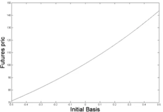
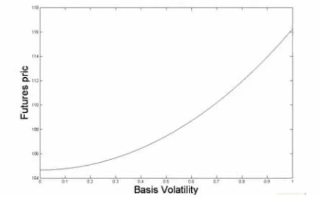
(7) Chou-Wen Wang and Ting-Yi Wu. 127. expectation of the futures price is a function of the spot price, volatility of the spot return, initial basis, and basis volatility. Second, the basis is modeled directly without regard to the appropriate number of state variables in a futures contract. Third, the basis is not only stochastic but also has a zero value at the maturity of the futures contract. The Brownian bridge process describes the convergence behavior of the spot price and the futures price quite well at the expiration of the futures contract. The features of the futures model with basis risk are presented graphically by numerical analysis in the next section. 3. Numerical Analysis. To investigate the properties of the FBR model, numerical results are illustrated in Figures 1 and 2. The numerical analysis focuses on the effects of the basis risk, rather than the effects of the spot price, on the futures price. Therefore, only the two parameters of initial basis and basis volatility are used to assess the impact of the basis risk on the futures price. The effects of the parameters for the spot price and interest rate on the futures price have been investigated by other researchers. Therefore, these factors are not mentioned in the current study. Figure 1 shows the relation between the futures price and the initial basis Z (0, T ) . Let the futures prices be computed using S (0) = 100 , r = 0.03 , δ = 0.015 , T = 0.5 , t = 0.3 , σ Z = 0.09 , and Z (0, T ) , which ranges from −0.5 to +0.5. Here Z (0, T ) is defined as the log futures price minus the log spot price. When Z (0, T ) is a negative number, the futures market is an inverted market; otherwise, if Z (0, T ) is a positive value, it is a normal market. As shown, the solution for the futures price in (14) increases with respect to the initial basis. When the initial basis is less than zero, the futures price is also less than the spot price. Holding the spot price unchanged, a higher initial basis results in a higher futures price. In addition, the futures price is a function of the exponential of the initial basis, so it has growth on an upward curve. Figure 1. The Effect of the Initial Basis on the Price of Futures Contracts. Figure 2 shows the impact of basis volatility σ Z on the futures price. Let Z (0, T ) = 0.05 , σ Z range from 0 to 1, and the values of other parameters remain.

(8) 128. International Journal of Business and Economics. the same as above. In Figure 2, the futures price in (14) increases with respect to the basis volatility. This suggests that the holder of the futures contract should be compensated for taking risk when the basis volatility is high. The numerical analysis suggests that the initial basis and basis volatility have significant and positive impacts on the futures price. The next section provides empirical evidence for the occurrence of basis risk in stock futures and assesses the performance of the FBR model using S&P 500 futures. Figure 2. The Effect of the Basis Volatility on the Price of Futures Contracts. 4. Empirical Test. This section includes an empirical test of the performance of the FBR model. The CF and Yan models are used to assess the efficiency of the FBR model. The CF model is the model of non-basis risk. The basis risk is the only difference between the FBR and CF models, so if the FBR model can significantly improve the biases and goodness-of-fit created by the CF model, we can determine the existence of basis risk. The Yan (2002) model is used to perform another empirical test of a general futures model that incorporates most stochastic factors investigated in the futures literature. The FBR model directly formulates the basis as an exogenous stochastic process, while Yan’s model indirectly formulates the basis through the stochastic convenience yield, stochastic interest rate, stochastic volatility, and simultaneous jumps in the spot price and volatility. The comparison can empirically assess which pricing approach is more efficient. 4.1 Empirical Data. The empirical test of the FBR model is carried out using daily traded prices of the S&P 500 Composite Price Index and the S&P 500 futures on the Chicago Mercantile Exchange from January 2, 1991, to June 6, 2007. The data were chosen since the futures have great liquidity in the US and these sources are used pervasively in the existing literature (Lim and Guo, 2000)..

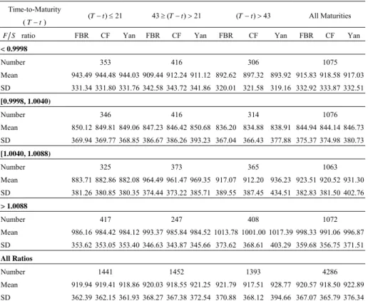
(9) Chou-Wen Wang and Ting-Yi Wu. 129. There are 4,286 futures prices in the sample, and all the futures contracts in the sample are nearby contracts. They are quoted in index points and range from 312.65 to 1,555.40. The risk-free rate is the secondary market rate of US 3-Month Treasury Bills provided by the Federal Reserve Bank of Saint Louis. These data are used to estimate the parameters and compute the model prices. 4.2 Parameter Estimation. To implement the futures pricing model, some unobservable parameters must be estimated using the observed traded futures prices in the sample data. For simplicity, the parameters are assumed to be constant. However, monthly estimations greatly increase the fit; therefore, we follow the spirit of many existing empirical models and use this method (Bakshi et al., 1997; Chang et al., 1998; Lim and Guo, 2000). For the FBR model, the parameters of the process σ S , a , σ Z , and Z (0, T ) must be estimated from the realized data. However, σ S is the only parameter that needs to be estimated in the CF model. For Yan’s model, the parameters of the process σ S , θ r , κ r , and σ r (defined in Yan, 2002) must be estimated from the realized daily data. 4.3 Test of Model Performance. The performance of the FBR model is examined using an empirical test. We divided time-to-maturity into three groups and the F S ratio into four groups. Including both the subtotals and the grand total, there are 20 groups. We show the mean error (ME), mean absolute error (MAE), and root mean square error (RMSE) statistics in terms of both index points and percentage in order to assess the efficiency of the three competing futures models. The index point error is defined as the difference between the model price and the actual price. The percentage error is the index point error divided by the actual price: eindex = Fmo − Factual e per =. eindex × 100% , Factual. (18) (19). where Fmo is the model price of future contract, Factual is the actual price of the futures contract, eindex is the index point error, and e per is the percentage error. The empirical test assesses the performance of the model prices compared to the actual prices using the parameters estimated from the realized data in the same month. The time-to-maturity and F S ratio biases are examined to analyze the magnitude of misspecification. Table 1 presents descriptive statistics for the futures prices calculated for the FBR, CF, and Yan models, respectively. The prices computed by Yan’s model are larger than those of the FBR and CF models in most cases. For the grand total group, the Yan model has the highest average model price (922.89), while the CF model has the lowest average model price (918.50)..

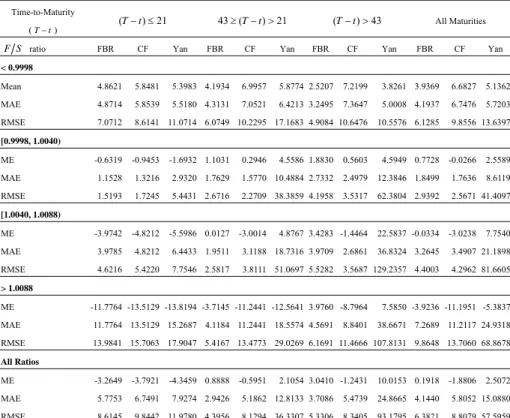
(10) 130. International Journal of Business and Economics Table 1. Descriptive Statistics. Time-to-Maturity (T −t ) F S ratio. (T − t ) ≤ 21. FBR. CF. 43 ≥ (T − t ) > 21. Yan. FBR. CF. Yan. (T − t ) > 43. FBR. CF. All Maturities Yan. FBR. CF. Yan. < 0.9998 Number. 353. 416. 306. 1075. Mean. 943.49 944.48 944.03 909.44 912.24 911.12 892.62 897.32 893.92 915.83 918.58 917.03. SD. 331.34 331.80 331.76 342.58 343.72 341.86 320.01 321.58 319.16 332.92 333.87 332.51. [0.9998, 1.0040) Number. 346. 416. 314. 1076. Mean. 850.12 849.81 849.06 847.23 846.42 850.68 836.20 834.88 838.91 844.94 844.14 846.73. SD. 369.94 369.77 368.85 386.67 386.26 393.23 367.04 366.43 377.88 375.37 374.98 380.73. [1.0040, 1.0088) Number. 325. 373. 365. 1063. Mean. 883.71 882.86 882.08 964.49 961.47 969.35 917.07 912.20 936.23 923.51 920.52 931.30. SD. 381.26 380.85 380.35 374.44 373.22 385.71 389.55 387.45 434.51 382.83 381.50 402.76. > 1.0088 Number. 417. 247. 408. 1072. Mean. 986.16 984.42 984.12 993.37 985.84 984.52 1013.78 1001.00 1017.39 998.33 991.06 996.87. SD. 353.62 353.05 353.40 346.63 343.87 345.66 373.62 368.61 403.29 359.68 356.75 371.51. All Ratios Number. 1441. 1452. 1393. 4286. Mean. 919.94 919.41 918.86 920.03 918.55 921.25 921.79 917.51 928.77 920.57 918.50 922.89. SD. 362.39 362.15 361.93 368.27 367.38 372.54 370.88 368.12 394.66 367.07 365.79 376.34. The empirical results in index points and percentage terms are presented in Tables 2 and 3, respectively. The FBR model shows better goodness-of-fit with no significant evidence of biases related to the time-to-maturity or F S ratio. In contrast, the CF and Yan models displayed worse goodness-of-fit with evidence of time-to-maturity and F S ratio biases. Bias The overall empirical performances showed no significant biases for the FBR model, but Yan’s model showed significant biases and the CF model displayed a certain degree of bias. The mean error of the FBR model is smallest in terms of index points and the percentage of all futures in the sample. For the grand total group, the mean error is 0.1918 and −0.002% for the FBR model, −1.8806 and −0.2088% for the CF model, and 2.5072 and 0.0973% for the Yan model. The mean error of the FBR model in index points is 10 and 13 times smaller than those of the CF and Yan models, respectively. There is no significant time-to-maturity or F S ratio bias for the FBR model. However, the CF and Yan models displayed significant biases in terms of both the time-to-maturity and F S ratio. In both the F S ratio and time-to-maturity, the.

(11) 131. Chou-Wen Wang and Ting-Yi Wu. Yan model generally overestimated the futures price (shown by a positive mean error), but the CF model underestimated the futures price (shown by a negative mean error) in most groups. Moreover, there are two obvious patterns in Table 2: (1) the degree of mispricing for the CF model was positively proportional to the F S ratio, i.e., the futures prices were underpriced more severely when the F S ratio was increasing and (2) Yan’s model overpriced the futures prices more severely when the time-to-maturity was farther away. The bias was evident according to the mean errors for both index points and percentage. Table 2. Empirical Test Results: Index Point Errors Time-to-Maturity. (T − t ) ≤ 21. ( T −t ). F S ratio. FBR. CF. 43 ≥ (T − t ) > 21 Yan. FBR. CF. Yan. (T − t ) > 43 FBR. CF. All Maturities Yan. FBR. CF. Yan. < 0.9998 Mean. 4.8621. 5.8481. 5.3983 4.1934. 6.9957. 5.8774 2.5207. 7.2199. 3.8261 3.9369. 6.6827. 5.1362. MAE. 4.8714. 5.8539. 5.5180 4.3131. 7.0521. 6.4213 3.2495. 7.3647. 5.0008 4.1937. 6.7476. 5.7203. RMSE. 7.0712. 8.6141 11.0714 6.0749 10.2295 17.1683 4.9084 10.6476. 10.5576 6.1285. 9.8556 13.6397. [0.9998, 1.0040) ME. -0.6319. -0.9453. -1.6932 1.1031. 4.5586 1.8830. 0.5603. 4.5949 0.7728. -0.0266. 2.5589. MAE. 1.1528. 1.3216. 2.9320 1.7629. 1.5770 10.4884 2.7332. 0.2946. 2.4979. 12.3846 1.8499. 1.7636. 8.6119. RMSE. 1.5193. 1.7245. 5.4431 2.6716. 2.2709 38.3859 4.1958. 3.5317. 62.3804 2.9392. 2.5671 41.4097. -3.9742. -4.8212. -5.5986 0.0127. 4.8767 3.4283 -1.4464. 22.5837 -0.0334. [1.0040, 1.0088) ME. -3.0014. -3.0238. 7.7540. MAE. 3.9785. 4.8212. 6.4433 1.9511. 3.1188 18.7316 3.9709. 2.6861. 36.8324 3.2645. 3.4907 21.1898. RMSE. 4.6216. 5.4220. 7.7546 2.5817. 3.8111 51.0697 5.5282. 3.5687 129.2357 4.4003. 4.2962 81.6605. > 1.0088 ME. -11.7764 -13.5129 -13.8194 -3.7145 -11.2441 -12.5641 3.9760 -8.7964 8.8401. 7.5850 -3.9236 -11.1951 -5.3837. MAE. 11.7764 13.5129 15.2687 4.1184 11.2441 18.5574 4.5691. 38.6671 7.2689 11.2117 24.9318. RMSE. 13.9841 15.7063 17.9047 5.4167 13.4773 29.0269 6.1691 11.4666 107.8131 9.8648 13.7060 68.8678. All Ratios ME. -3.2649. -3.7921. -4.3459 0.8888. MAE. 5.7753. 6.7491. 7.9274 2.9426. -0.5951. 5.1862 12.8133 3.7086. 2.1054 3.0410 -1.2431 5.4739. 24.8665 4.1440. 10.0153 0.1918. -1.8806. 5.8052 15.0880. 2.5072. RMSE. 8.6145. 9.8442 11.9780 4.3956. 8.1294 36.3307 5.3306. 8.3405. 93.1795 6.3821. 8.8079 57.5959. In addition, the relative magnitude of the MAE with respect to the absolute ME in index points was larger in most subcategories in the FBR model than in the CF and Yan models. For example, in the grand total group of Table 2, the CF model generated an MAE of 5.8055 and an ME of −1.8806, while the Yan model generated 15.088 and 2.5072 and the FBR model generated 4.144 and 0.19183. Taking MAE/ME (Lim and Guo, 2000), we obtain 3 for the CF model, 6 for the Yan model, and 21 for the FBR model. This can also be interpreted as evidence of bias in the CF and Yan models. When most of the errors are of the same sign in each subgroup, the ME is close to the MAE in index points, and vice versa. The prices of the FBR model are closer around the actual prices, so the ME is much smaller than the MAE in index terms..

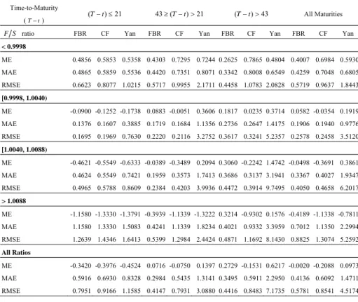
(12) 132. International Journal of Business and Economics Table 3. Empirical Test Results: Percentage Errors. Time-to-Maturity. (T − t ) ≤ 21. ( T −t ). F S ratio. FBR. CF. 43 ≥ (T − t ) > 21 Yan. FBR. CF. Yan. (T − t ) > 43 FBR. CF. All Maturities Yan. FBR. CF. Yan. < 0.9998 ME. 0.4856 0.5853 0.5358 0.4303 0.7295 0.7244 0.2625 0.7865 0.4804 0.4007 0.6984 0.5930. MAE. 0.4865 0.5859 0.5536 0.4420 0.7351 0.8071 0.3342 0.8008 0.6549 0.4259 0.7048 0.6805. RMSE. 0.6623 0.8077 1.0215 0.5717 0.9955 2.1711 0.4458 1.0783 2.0828 0.5719 0.9637 1.8443. [0.9998, 1.0040) ME. -0.0900 -0.1252 -0.1738 0.0883 -0.0051 0.3606 0.1817 0.0235 0.3714 0.0582 -0.0354 0.1919. MAE. 0.1376 0.1607 0.3885 0.1719 0.1684 1.1356 0.2736 0.2647 1.4175 0.1906 0.1940 0.9776. RMSE. 0.1695 0.1969 0.7630 0.2220 0.2116 3.2752 0.3617 0.3241 5.2357 0.2578 0.2458 3.5120. [1.0040, 1.0088) ME. -0.4621 -0.5549 -0.6333 -0.0389 -0.3489 0.2094 0.3060 -0.2242 1.4742 -0.0498 -0.3691 0.3861. MAE. 0.4624 0.5549 0.7421 0.1959 0.3573 1.7413 0.3686 0.3137 3.1941 0.3367 0.4027 1.9347. RMSE. 0.4965 0.5788 0.8609 0.2384 0.4203 3.9936 0.4472 0.3914 9.7495 0.4050 0.4658 6.2017. > 1.0088 ME. -1.1580 -1.3330 -1.3791 -0.3939 -1.1339 -1.3222 0.3214 -0.9302 0.1576 -0.4189 -1.1338 -0.7811. MAE. 1.1580 1.3330 1.5083 0.4241 1.1339 1.8234 0.4021 0.9332 3.3959 0.7012 1.1350 2.2994. RMSE. 1.2639 1.4346 1.6413 0.5399 1.2984 2.4424 0.4871 1.1692 8.1430 0.8825 1.3074 5.2592. All Ratios ME. -0.3420 -0.3976 -0.4524 0.0716 -0.0750 0.1397 0.2729 -0.1531 0.6217 -0.0020 -0.2088 0.0973. MAE. 0.5916 0.6930 0.8328 0.2984 0.5435 1.3141 0.3495 0.5911 2.2950 0.4136 0.6092 1.4711. RMSE. 0.7951 0.9166 1.1585 0.4147 0.7931 3.0880 0.4416 0.8483 7.1735 0.5781 0.8541 4.5174. Goodness-of-Fit The overall MAE in index terms is 4.144 for the FBR model, 5.8055 for the CF model, and 15.088 for the Yan model. In percentage terms, the overall MAE is 0.4136% for the FBR model, 0.6092% for the CF model, and 1.4711% for Yan’s model. This is consistent with the RMSE statistics. The FBR model is superior to the CF and Yan models in most categories. The MAE and the RMSE are reported to measure each model’s goodness-of-fit. The MAE gives the sense of expected average error, while the RMSE punishes larger errors because they receive more weight when squared, so it is more appropriate for use with risk-averse investors. By both measures, the FBR shows better goodness-of-fit. The smaller bias and better goodness-of-fit in the empirical test for the FBR model shows that: (1) there is evidence of basis risk in S&P 500 futures and (2) the FBR model directly formulates the basis as an exogenous stochastic process, while the Yan model indirectly formulates the basis using factors investigated in the futures literature. The pricing approach in the FBR model is more efficient than that in Yan’s model. The theoretical assumptions about a futures price, which is affected by the underlying asset and the basis, is, therefore, supported by empirical results..

(13) Chou-Wen Wang and Ting-Yi Wu. 133. 5. Conclusion. This study formulates an alternative futures model that differs from the Cornell and French (1983a) and Yan (2002) models by assuming that the futures price is a function of underlying assets and basis risk, which follows a Brownian bridge process. This assumption does not require us to determine the appropriate number of state variables in a futures model. In addition, the basis is modeled directly as an exogenous stochastic process that has a zero value at the maturity of the futures contract. The basis follows a Brownian bridge that describes the convergence behavior of the spot price and the futures price quite well at the expiration of the futures contract. The FBR model is empirically tested using daily data on the S&P 500 composite price index and S&P 500 futures. Compared with the Cornell and French (1983a) and Yan (2002) models, the empirical test provides evidence that supports the occurrence of basis risk in a futures model. In addition, the Yan (2002) model has an over-sufficiency of information to estimate the futures price. The FBR model outperformed the CF and Yan models by producing a smaller bias, eliminating the F S ratio and time-to-maturity biases and demonstrating a better goodness-of-fit. In most categories, the mean errors in terms of both index points and percentages are much smaller for the FBR model than for the CF and Yan models. The futures model with basis risk gives an exact formula that provides greater accuracy and is useful for developing stock index futures. Appendix Proof of Proposition 1. According to the Girsanov theorem in (7), the basis process Z (t , T ) defined in (10) can be written as: − Z (t , T ) dt + σ% Z (t , T ) ⎡⎣ dW T (t ) + b (t , T ) dt ⎤⎦ T −t ⎡ − Z (t , T ) ⎤ =⎢ + σ% Z (t , T ) ⋅ b (t , T ) ⎥ dt + σ% Z (t , T ) dW T (t ). ⎣ T −t ⎦. dZ (t , T ) =. (A-1). To obtain the solution of Z (t , T ) , we use the technique presented in Klebaner (1998, p. 121). Consider the general linear SDE: dZ (t , T ) = [α (t ) + β (t ) Z (t , T ) ] dt + [γ (t ) + ϕ (t ) Z (t , T ) ] dW (t ) ,. (A-2). where the functions α , β , γ , and ϕ are given and adapted processes and are continuous functions of t . Then Z (t , T ) is found to be: t α ( u ) − ϕ ( u )γ ( u ) t γ (u ) ⎡ ⎤ Z (t , T ) = X (t ) ⎢ Z (0, T ) + ∫ du + ∫ dW (u ) ⎥ , 0 0 X (u ) X (u ) ⎣ ⎦. (A-3).

(14) 134. International Journal of Business and Economics. where X (t ) is the stochastic exponential SDE and: dX (t ) = β (t )X (t ) dt + ϕ (t )X (t ) dW (t ) .. From (A-1) and (A-2), we have α (t ) = σ% Z (t , T ) ⋅ b(t , T ) , β (t ) = −1 T − t , γ (t ) = σ% Z (t , T ) , and ϕ (t ) = 0 . Let X (0) = 1 . From the previous condition, we use (A-3) to obtain (12). References. Bakshi, G., C. Gao, and Z. Chen, (1997), “Empirical Performance of Alternative Option Pricing Models,” Journal of Finance, 52, 2003-2049. Chang, C., J. Chang, and K. G. Lim, (1998), “Information-Time Option Pricing: Theory and Empirical Evidence,” Journal of Financial Economics, 48, 211-242. Cornell, B. and K. R. French, (1983), “The Pricing of Stock Index Futures,” The Journal of Futures Markets, 3(1), 1-14. Cox, J. C., J. E. Ingersoll, and S. A. Ross, (1985), “A Theory of the Term Structure of Interest Rates,” Econometrica, 53, 384-407. Gibson, R. and E. Schwartz, (1990), “Stochastic Convenience Yield and the Pricing of Oil Contingent Claims,” Journal of Finance, 45, 959-976. Gujarati, D. N., (2003), Basic Econometrics, 4th edition, New York: Mc Graw Hill, Inc. Hemler, M. L. and F. A. Longstaff, (1991), “General Equilibrium Stock Index Futures Prices: Theory and Empirical Evidence,” Journal of Financial and Quantitative Analysis, 26(3), 287-308. Hilliard, J. and J. Reis, (1998), “Valuation of Commodity Futures and Options under Stochastic Convenience Yields, Interest Rates, and Jump Diffusions in the Spot,” Journal of Financial and Quantitative Analysis, 33(1), 61-86. Klebaner, F., (1998), Introduction to Stochastic Calculus with Applications, London: Imperial College Press, Inc. Lim, K. G. and X. Guo, (2000), “Pricing American Options with Stochastic Volatility: Evidence from S&P 500 Futures Options,” Journal of Futures Markets, 20, 625-659. Miltersen, K. and E. Schwartz, (1998), “Pricing of Options on Commodity Futures with Stochastic Term Structures of Convenience Yields and Interest Rates,” Journal of Financial and Quantitative Analysis, 33(1), 33-59. Ramaswamy, K. and S. M. Sundaresan, (1985), “The Valuation of Options on Futures Contracts,” Journal of Finance, 40, 1319-1340. Schwartz, E. S., (1997), “The Stochastic Behavior of Commodity Prices: Implications for Valuation and Hedging,” Journal of Finance, 52, 922-973. Yan, X., (2002), “Valuation of Commodity Derivatives in a New Multi-Factor Model,” Review of Derivatives Research, 5, 251-271..

(15)