https://doi.org/10.1007/s00366-019-00759-4
ORIGINAL ARTICLE
A heuristic moment‑based framework for optimization design
under uncertainty
Kuo‑Wei Liao1 · Nophi Ian D. Biton2
Received: 4 December 2018 / Accepted: 22 April 2019 © Springer-Verlag London Ltd., part of Springer Nature 2019
Abstract
To search an optimal design under uncertainty, this study proposes an effective framework that integrates the moment-based reliability analysis into a heuristic optimization algorithm. Integration of an equivalent single-variable performance function is an ideal concept to calculate the failure probability. However, such integration is often not available and is alternatively computed using the first four moments and a generalized moment-based reliability index is established, in which the Gauss-ian–Hermite integration and dimension reduction are implemented to enhance the effectiveness. To overcome the limited applicable range of moment-based approach, an adjustable optimization procedure is proposed, in which different reliability methods are performed depending on results of the constraint assessments. In addition, the ε level comparison is integrated into particle-swarm optimization to consider the constraint violation. Several literature studies are used to verify the accuracy of the proposed optimization framework including problems having linear, highly nonlinear, implicit probabilistic constraint functions with normal or non-normal variables and system-level reliability analysis. The effects of several parameters, such as the number of estimate point, the number of dimension, and the degree of uncertainty, are thoroughly investigated. Results indicating that tri-variate with seven points are able to provide a stable solution under a high degree of uncertainty.
Keywords Risk and reliability · Safety · Uncertainty · Probabilistic design · Optimization techniques
1 Introduction
Uncertainties in an engineering design problem are often inevitable; to ensure a greater performance, reliability-based design optimization (RBDO) is often adopted. A traditional RBDO is a nested double-loop approach in which the outer loop is the deterministic optimization, and the inner loop is the reliability analysis, which is often a barrier in appli-cation. To simplify the computational complexity of an RBDO problem, many algorithms have been proposed. For example, safety factor has been adopted in many design codes to take uncertainties into consideration. The safety factor approach, however, often fails to identify the relative
importance among design parameters, because all uncertain-ties are represented by s single factor throughout the design [11]. Du and Chen [2] proposed the sequential optimization and reliability assessment (SORA) to sequentially conduct the deterministic optimization and inverse reliability analysis until the solution converges. Liao and Ha [10] incorporated a reliability analysis of mean value method with an SORA to further improve efficiency of an RBDO solution. Mean value method is a first-order Taylor’s expansion using mean value as the expansion point, which is a simplified approach and is suitable for a problem without highly nonlinear performance functions. Li et al. [9] considered an SORA problem using hybrid uncertainty, which is described by randomness and fuzziness. This approach is specially designed for a problem with different cognitive levels to various uncertain param-eters. Yi et al. [26] proposed a method that approximately estimated the most probable point (MPP) and probabilistic performance measure in reliability assessment to improve the efficiency of SORA. In their approach, evaluation of performance function in the deterministic optimization is not needed and, therefore, reducing the computational time. Raza and Liang [17] also utilized the similar concept to * Kuo-Wei Liao
[email protected] Nophi Ian D. Biton [email protected]
1 Department of Bioenvironmental Systems Engineering, National Taiwan University, Taipei, Taiwan
2 University of San Carlos-Cebu, Cebu City, Philippines
decouple the reliability analysis in a traditional double-loop RBDO optimization task. Liu and Zhang [13] utilized the decoupling strategy to develop an equivalent single-layer optimization model that is solved by the sequential quadratic programming (SQP) method. The benefit of this approach is similar to SORA, in which a decoupling strategy was devel-oped to solve the nesting optimization problem, alleviating the computational burden.
Other than decoupling approach, Mansour and Olsson [14] adopted the response surface methodology in solv-ing an RBDO problem, which is particularly useful for the industrial applications due to the use of the finite-element software. Shan and Wang [18] converted the double-loop RBDO into a single-loop procedure, in which a deterministic optimization problem is formulated and constrained by a reliable design space rather than the original deterministic feasible space. In balancing the computational cost and the accuracy of the reliability assessment, this study incorpo-rates the methods of moments [13, 27, 28, 30, 31] as the reliability analysis procedure and particle-swarm optimiza-tion (PSO) for solving RBDO problems.
Many gradient-based optimization algorithms have been proposed in the literature [5–7, 22]. For a gradient-based approach (e.g., SQP), derivatives of the objective and con-straint functions are needed to find the optimal direction and step in the next iteration. However, derivative calcu-lations could be an obstacle for non-differentiable cases. Recently, heuristic optimization algorithm such as the PSO has been proposed and drawn many attentions [3, 5, 22]. Because derivatives are not needed in PSO, PSO is adopted this study. Similar to optimization, many algorithms have been proposed to estimate the failure probability for a given performance function. The first-order reliability analysis (FORM) and the Monte Carlo simulation (MCS) are two frequently approaches. FORM computes the failure prob-ability through an optimization procedure, in which the goal is to find the minimal distance between the origin and the limit-state function in the standard normal and uncorrelated random variable space. The limit-state function is defined as g = 0, where g is the performance function. The point on the limit-state corresponding to this minimum distance is called the MPP. The shortest distance is called reliability index (β) with a corresponding failure probability. MCS, on the other hand, is a sampling-based approach, relying on repeated random sampling to obtain the failure probability. If the failure probability is very small, which is often found in an engineering design problem, a large sample size is often required. Both FORM and MCS are easily to be integrated into the RBDO. However, the accuracy of the FORM and the computational cost of MCS are two major concerns if such approach is adopted.
This study incorporates the methods of moments with PSO to solve an RBDO problem. Failure probability is the integral
of the performance function under a given probability density function (PDF). In reality, the PDF of a performance function is often not available. The first few central moments, calcu-lated by point estimates in the standard normal space, are used to compute the probability of failure in the proposed RBDO approach. A generalized multivariate dimension-reduction method proposed by Xu and Rahman [25] is utilized to con-sider a performance function with multiple random variables. Details of the proposed algorithm are described in the follow-ing sections.
2 The reliability analyses used in the current
study: methods of moments [
29
]
The failure probability (PF) of a given performance (G) is the
integration of
where X are the random variables considered and fx is the
PDF of X. If the performance function can be represented by a PDF with a single variable of Z, the integration described in Eq. (1) can solved as described in the following equation:
where Zs is the standardization of Z, and σG and μG are
stand-ard deviation and mean value of the performance function, respectively. β2M are the second moment reliability index. Similar to the Rosenblatt transformation, assuming that the CDFs of Zs and standard normal (U) are equal, then one can
establish the relationship of the standardized variable and standard normal variable using the first few moments of Z, as described in the following equation:
where S−1 is the inverse function of S and M is the first few
moments of Z. A general moment-based reliability index can be derived, as described in the following equation:
(1) PF= P(Z = G(𝐗) ≤ 0) = � G(𝐗)≤0 fx(x)dx, (2) ⎧ ⎪ ⎪ ⎨ ⎪ ⎪ ⎩ PF= P(Z≤ 0) = P(𝜎GZS+ 𝜇G≤ 0) = P � ZS ≤ −𝜇G 𝜎G � PF= P(ZS≤ −𝛽2M) = � −𝛽2M −∞ fZ s(Zs)dzs, (3) Zs= S(U, 𝐌) U= S−1(Zs, 𝐌), (4) FZ s = 𝛷(u) = 𝛷[S −1(z s, 𝐌)] PF= FZs(−𝛽2M) = 𝛷[S −1(−𝛽 2M, 𝐌)] 𝛽 = −𝛷−1(P F) = −S−1(−𝛽2M, 𝐌).
Thus, the remaining tasks of reliability analysis are to find the inverse function S−1 and the moments of the
per-formance function (M). The calculation of moments of the performance is first described below.
2.1 Point estimation and dimension reduction Estimating moments for a performance function in a stand-ard normal space is conceptually identical to Gaussian–Her-mite integration. In this study, the kth moment of a per-formance function, G(X), is estimated, as described in the following equation:
where ϕ is the standard normal probability density function,
u is standard normal variable, Pj and uj are the weight and
point, m is the number of point, and z(u) is expressed in the following equation:
where T is the Rosenblatt transformation function, and k is the kth moment under estimation. There are two different ways of standardizing the Hermite polynomials: the “proba-bilists’ Hermite polynomials” and the “physicists’ Hermite polynomials”. These two definitions are related to each other through the following equation:
where Hm is the physicists’ Hermite polynomials and Hem is the probabilists’ Hermite polynomials. The weights of the physicists’ Hermite polynomials are given as follows:
Compared to the physicists’ Hermite polynomials, the probabilists’ Hermite polynomials are closer to Eq. (5) that is used to estimate moments for a performance function in a standard normal space in the current study. By compar-ing Eq. (5) and the integration using probabilists’ Hermite polynomials, Eq. (9) can be derived:
With Eqs. (7) and (9), the weights (Pj) in Eq. (5) can be
derived and is described in the following equation: (5) ∫ z(u)𝜙(u)du = m ∑ j=1 Pjz(uj), (6) z(u) = {G[T(−1)(U)] − 𝜇G} k , (7) Hm(x) = 2m2H em �√ 2x � , (8) wj= 2 m−1m!√𝜋 m2H2 m−1(xj) . (9) Pj= √1 𝜋wj. (10) Pj= m! m2H2 em−1(uj) ,
where Hem is the probabilists’ Hermite polynomials, and uj
is the abscissas of the Hermite polynomials.
For a function of many variables, a generalized multivari-ate dimension-reduction method proposed by Xu and Rah-man [25] is adopted here. The multivariate approximation,
G’, consists of all terms of the Taylor series expansion of an N-dimensional, G(X), that have no more than D variables
(D ≤ N). That is, for G(X) = G(x1, x2,… , xN) , a D-variate
approximation G’ is given in the following equation:
where GD defines a summation of terms that contain at most
D variables, as given in the following equation:
After applying the D-variate approximation, the point estimate procedure for a single variable described in Eq. (5) is then used to compute the first fourth moments of G(X), as shown in the following equation:
where 𝜇kG (k=1, 2, 3, 4) refers to the kth moments about zero
that is defined in the following equation:
2.2 Third‑ and fourth‑moment reliability methods Following the assumption of Tichy [21], the standardized variable Zs is described by the three-parameter lognormal
distribution, the third-moment reliability index based on Eqs. (3) and (4) is provided in the following equation:
where 𝛼3G is the third dimensionless central moment, i.e., the
skewness of Z = G(X). Zhao and Ono [28] assumed that Zs
follows the 3P square normal distribution, the third-moment reliability index following Eqs. (3) and (4) can be expressed as
(11) G�= D ∑ i=0 (−1)i ( N− S + i − 1 i ) GD−i, (12) GD= ∑ k1<k2<⋯<kD G(0, … , 0, xk 1, 0, … , 0, xk2, 0, … , 0, xkD, 0, … , 0), 0≤ D ≤ N. (13) ⎧ ⎪ ⎪ ⎨ ⎪ ⎪ ⎩ 𝜇G= 𝜇1G 𝜎G= � 𝜇2G− 𝜇2 1G 𝛼3G= (𝜇3G− 3𝜇2G𝜇1G+ 2𝜇3 1G)∕𝜎 3 G 𝛼4G= (𝜇4G− 4𝜇3G𝜇1G+ 6𝜇2G𝜇2 1G− 3𝜇 4 1G)∕𝜎 4 G , (14) 𝜇kG = ∫ +∞ −∞ ⋯∫ +∞ −∞ {G[T(−1)(u)]}k𝜙(u)du. (15) 𝛽3M−L= −𝛼3G 6 − 3 𝛼3Gln ( 1−1 3𝛼3G𝛽2M ) , (16) 𝛽3M−S= 1 𝛼3G ( 3− √ 9+ 𝛼2 3G− 6𝛼3G𝛽2M ) .
Wang et al. [23] proposed another third-moment reliability index that has a wider applicable range and less limitation compared to that of Eqs. (15) and (16), as shown in Eq. (17), which is obtained by fitting the average value of 𝛽3M−L and
𝛽3M−S:
Equation (17) is implemented in the proposed RBDO when the fourth-moment method is not applicable. It is observed that the third-moment reliability index becomes undefined when
β2M is equal to zero. Nevertheless, it is very unusual to encoun-ter such a case in a practical engineering problem. The afore-mentioned 3M approaches are approximate methods and the applicable range of 𝛼3G (if r = 2%, r is the allowable relative
error between 𝛽3M−L and 𝛽3M−S ) is described in Eq. (18) [31]:
It is noted that the 3M method is more suitable for nega-tive values of skewness, since the probability of failure is
(17) 𝛽3M−W = 1 3𝛽2M [ 2+ e 1 2𝛼3G ( 𝛽2M− 1 𝛽2M )] . (18) −2.4∕𝛽2M≤ 𝛼3G≤ 0.8∕𝛽2M.
integrated in the left tail of the PDF. Based on the U − Zs
transformation provided by Fleishman [4], as shown in the following equation:
in which ai (i = 1, 2, 3, 4) are deterministic coefficients.
The 4M reliability index can be established which is briefly described in the following. Assuming that the first four cen-tral moments of U and Zs are the same, one can find a2 and
a4 through the following equation:
where Ai= hi(a2, a4) , hi (i = 1, 2, 3, 4) are polynomial
func-tions. Once a2 and a4 are obtained, a1 and a3 can be solved using the following equation:
The 4M reliability index based on Eqs. (3) and (4) is pro-vided in the following equation:
(19) ZS= a1+ a2U+ a3U2+ a4U3, (20) 2A1A2= 𝛼23G 3A1A3+ 3A4 = 𝛼4G, (21) a3= −a1= 𝛼3G 2A2 . (22) 𝛽4M−C= P D− D + a3 3a4, where
Similarly, an applicable range of 𝛼4G is provided in
Eq. (23) [30] which is used to determine whether the 4M reliability is applied or not in our proposed RBDO approach. Details are provided in “The proposed RBDO”:
Zhao et al. [32] developed a complete expression of the fourth-moment normal transformation including six cases with different combinations of skewness and kurtosis. The applicable ranges are provided below:
D= 3 � Δ − q 2 ,Δ = √ q2+ 4p3, p= 3a2 a4− a2 3 9a2 4 , q= 2a3 3− 9a2a4a3 27a3 4 + a1+ 𝛽2M a4 . (23) 2.9+ 𝛼3G2 ≤ 𝛼4G≤ 5.2 + 𝛼3G2 . (24) { abs(1.9 − 0.0649𝛼3G+ 1.5988𝛼2 3G)≤ 𝛼4G≤ abs(3.1 − 0.45𝛼3G+ 1.6111𝛼23G) if a4< 0 abs(3.1 − 0.45𝛼3G+ 1.6111𝛼2 3G)≤ 𝛼4G≤ 7 if a4≥ 0 .
Equation (24) is used for the first three examples for comparison. For details, please refer Sect. 6.
2.3 Methods of moments for system reliability In reality, a structure usually has multiple failure modes. The calculation of the failure probability for a system is necessary; however, it is generally not an easy task. If a moment-based reliability approach is adopted, one of the difficulties is in obtaining the mutual correlations among the failure modes. Several approaches have been proposed to lessen the computational burden of a system reliability problem. A moment-based method, in which the failure probability is evaluated without MCS and does not require the computation of the mutual correlations among failure modes, is adopted in the current study [27]. The perfor-mance function of a series system, G, is expressed as the minimum among each individual performance function, as indicated in the following equation:
where gi is the performance function of the ith failure mode.
Similarly, the performance function of a parallel system, G, is expressed as the maximum among each individual per-formance function, as indicated in the following equation:
(25)
G(𝐗) = min[g1, g2,… , gk],
(26)
For a combined series–parallel system, the performance function of the system then becomes a combination of maximum and minimum of the component performance functions. Once the system performance function and its corresponding central moments are identified, the reliabil-ity can be determined, as described in Sect. 2.
3 The proposed optimization: PSO
PSO was proposed by Eberhart and Kennedy [3]. PSO is an algorithm operating on the basis of a large population of solutions and has drawn many attentions due to it is simple and easy to adopt. To execute a PSO, a group of random numbers was used to initialize the entire population, consist-ing of a set of individual particles. Particle movements are influenced by the optimal experience of an individual parti-cle and that of the population. Weighted values are used to determine the degree of influence between the two. Random elements are also considered when determining the direc-tions of the particle movements, giving particles a chance to leave local trends and preventing them from being trapped within local optimums. Many variations have been proposed for PSOs. The following briefly describes the PSO used in this study. A new particle is generated using Eq. (27), as shown below:
where ⃗xi(t + 1) denotes the position of the ith particle in the
next iteration, ⃗xi(t) denotes the position of the ith particle in
the current iteration, and ⃗vi(t + 1) denotes the velocity of the
ith particle in the current iteration. The position of a particle
represents the values of that particle. The velocity of the ith particle is determined by the following equation:
where w is the inertia factor, ⃗vi(t) is the velocity at the
pre-vious iteration, ri (i = 1–2) are random numbers between 0
and 1, and c1 and c2 are the cognition and social factors,
respectively. ⃗xpBest is the particle position with the minimum
objective value in the ith population and ⃗xgBest is the
parti-cle position with the minimum objective value in the entire population.
Various strategies in constraint handling for PSO have been proposed. Takahama et al. [20] proposed the
ε-constrained PSO to improve the Deb’s comparison rules,
which is adopted in this study. If the constraint violation,
C(X), is less than a specified threshold, ε, the particle is
considered feasible. The constrained violation used in
ε-constrained PSO is given by Eqs. (29) and (30):
(27) ⃗xi(t + 1) = ⃗vi(t + 1) + ⃗xi(t), (28) ⃗vi(t + 1) = w × ⃗vi(t) + r1c1(⃗xpBest− ⃗xi(t)) + r2c2(⃗xgBest− ⃗xi(t)), (29) C(𝐗) = max { max j { 0, lj(𝐗) } , max j |||hj(𝐗)||| }
where lj is the jth inequality constraint, hj is the jth equality
constraint, and np is a positive number. It is seen that the constraint violation is given by the maximum of all con-straints or the sum of all concon-straints. The ε-constrained PSO uses a so-called “ε-level comparison” which is an order rela-tion of fitness value and constraint violarela-tion [f(X), ϕ(X)] to determine the pBest and gBest. The ε-level comparison, ≤ε, between (f1, ϕ1) and (f2, ϕ2) is defined by the following
equation:
Equation (31) indicates that the feasibility of X has higher priority than that of the fitness value.
4 The proposed RBDO
The proposed RBDO utilizes the second-, third-, or fourth-moment-based method with multivariate dimension-reduc-tion technique (e.g., univariate, bi-variate, and tri-variate) as the reliability analysis procedure and the PSO as the opti-mizer, named PSO-4M–3M–2M hereafter. The primary goal of the algorithm is to achieve the necessary accuracy with reasonable cost. As described in “Third- and fourth-moment reliability methods”, the third- and fourth-moment reliabil-ity indices are applicable in certain ranges. The reliabilreliabil-ity index (e.g., the second-, third-, or fourth moment-based) that gives better accuracy will be selected in our proposed RBDO. The accuracy of the moment-based reliability indi-ces usually follows:
1. Within the applicable range, the fourth-moment reliabil-ity index, β4M, is more accurate than other reliability indices.
2. The third-moment reliability index, β3M, within the
applicable range, is more accurate than the fourth-moment reliability index (β4M) that is out of the appli-cable range.
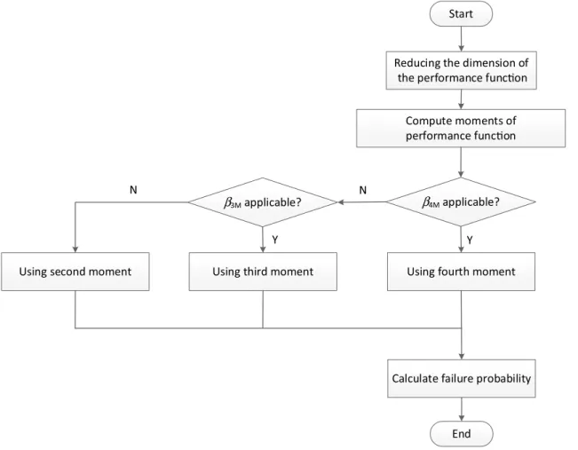
Based on the above observation, the reliability analysis procedure of this study is illustrated in Fig. 1 as described below.
1. Calculate the central moments of the performance func-tion using dimension-reducfunc-tion method.
(30) C(𝐗) =∑ j ‖‖ ‖max{0, lj(𝐗)}‖‖‖ p +∑ j ‖‖ ‖hj(𝐗)‖‖‖ np , (31) (f1, 𝜙1)≤𝜀(f2, 𝜙2) ⇔ ⎧ ⎪ ⎨ ⎪ ⎩ if 𝜙1, 𝜙2≤ 𝜀 and f1≤ f2, if 𝜙1 = 𝜙2and f1≤ f2 if 𝜀≤ 𝜙1≤ 𝜙2.
2. Calculate the applicable range of the third- and fourth-moment reliability indices.
3. If the fourth-moment reliability index is within the appli-cable range, then it is used as the reliability index. 4. If the fourth-moment reliability index is out of
applica-ble range, but the third reliability index is within appli-cable range, then the third-moment reliability index is used.
5. If the fourth- and third-moment reliability indices are not operable, then the second moment reliability index is used.
Figure 2 shows the detailed PSO evaluation process. For a given set of particles, the optimization process first com-putes particles’ position and velocity randomly. The fitness value and reliability index (based on Fig. 1) is then calcu-lated. The ε-constrained is used to update each particle’s pBest and gBest. If the predefined iteration number is not met, then update the velocity and position of each particle using Eqs. (27) and (28) for the next iteration.
All the demonstrated RBDO problems are employed in Intel Core i7 CPU 870 @ 2.93 GHz. The proposed algorithm
is coded in the Matlab 2013a version. The statistical tool-box is used here for the calculation of PDF and CDF of the different probability distributions. The SAP2000 is used to facilitate the structural analysis for the ten-bar truss prob-lem, in which the Open Application Programming Interface (OAPI) is developed to allow a third party software (such as MATLAB, the optimizer in the current study) to access the SAP2000 functions.
5 Numerical examples
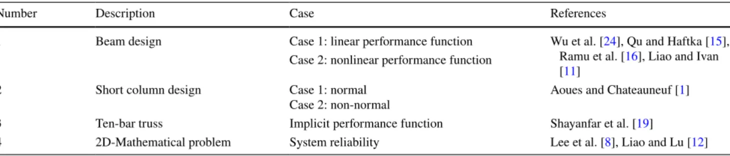
Several problems in the literature, as shown in Table 1, are used to examined the proposed RBDO algorithm. As indi-cated, different types of RBDO including linear and nonlin-ear performance functions, normal and non-normal variables, component and system reliability analyses are investigated. 5.1 Beam design
The objective of this optimization is to find the minimum weight or the minimum cross-sectional area of the cantilever
Start Compute moments of performance func on β4Mapplicable? End N
Using fourth moment Reducing the dimension of
the performance func on
Calculate failure probability Y
Using third moment Using second moment
β3Mapplicable?
N
Y
beam, as shown in Fig. 3. The width (w) and height (t) of the beam are considered as deterministic design variables. Two loads (FX, FY) at the free end, the modulus of elasticity (E),
and the yield strength (R) are considered as random design parameters.
The mathematical formulation of the RBDO problem is given in the following equation:
where w (in.) is the width, t (in.) is the depth, A (in.2) is the
area, PT
f is the target failure probability (i.e., 1.35 × 10⁻³), R
(psi) follows N(40,000, 2000) and is the allowable strength,
FX is an external horizontal force (lb) following N(500, 100),
and FY is an external vertical load (lb) following N(1000,
100). L (span) is 100 in. Do = 2.25 in. is the allowable tip
displacement. E (psi) is the elastic modulus which follows
N(29 × 106, 1.45 × . 106). Please note that the two
perfor-mance functions (G1 and G2) are separately considered (named case 1 and case 2). G1 is linear, while G2 is a
non-linear function. Nine-point estimation with three scenarios, univariate, bi-variate, and tri-variate dimension-reduction methods, is used in reliability analysis. 30 particles and 100 iterations are assigned in PSO, in which the values of c1 and
c2 are set to be 2.0. The velocity limit is imposed and a
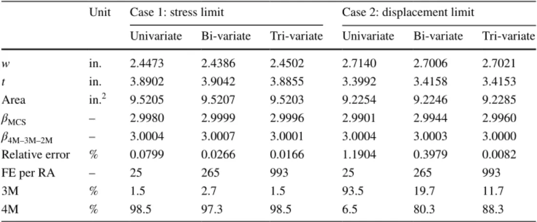
lin-early decreasing inertial parameter from 0.9 to 0.4 is used. Results using PSO-4M–3M–2M algorithm are shown in Tables 2, 3, and 4. For linear and nonlinear performance functions consisting of normal random variables, the PSO-4M–3M–2M is able to find the optimal design. The mean of the ten MCS runs with 106 samples is used to calculate the
relative error, which is described in the following equation:
where βMCS is the mean reliability index of ten independent MCS runs and β4M–3M–2M is the reliability index obtained
from the algorithm of PSO-4M–3M–2M. For both cases
Min.A= wt s.t. Prob.[Gi≤ 0] ≤ P T f 0≤ w, t ≤ 10 (32) G1(d, X) = R − (600∕(wt2)FY+ 600∕(w2t)FX) G2(d, X) = D0− (4L 3) Ewt √ ((FY∕t2)2+ (FX∕w2)2), (33) % error = | ̄𝛽MCS− 𝛽4M - 3M - 2M| ̄ 𝛽MCS , Start Generate par cles
Calculate fitness value
Calculate reliability index shown in Figure 1
Update pbest and gbest using the ε-level comparison
Reach predefined itera on No.
End N
Y
Calculate the constraint viola on
Fig. 2 Evaluation procedure of PSO in this study
Table 1 Summary of RBDO problems
Number Description Case References
1 Beam design Case 1: linear performance function Wu et al. [24], Qu and Haftka [15], Ramu et al. [16], Liao and Ivan [11]
Case 2: nonlinear performance function
2 Short column design Case 1: normal
Case 2: non-normal Aoues and Chateauneuf [1]
3 Ten-bar truss Implicit performance function Shayanfar et al. [19]
(i.e., the stress and displacement constraint), a decreasing trend in relative error is observed when a greater number of variates are used in dimension-reduction method. However, as expected, the function evaluation (FE) is increased in such approach. To be specific, the FE needed per reliability analy-sis is only 25 for univariate method, while it is 265 and 993 for the methods of bi-variate and tri-variate. With respect to the execution time of the univariate method, approximate three times and five times are needed for the methods of bi-variate and tri-bi-variate.
From Tables 3 and 4, it is observed that the results of PSO-4M–3M–2M are similar to that of the previous stud-ies. In general, the PSO-4M–3M–2M is able to find a better RBDO solution excepting the solution from Wu et al. [24]. Compared to the solutions of PSO-4M–3M–2M, earlier researches either have a bigger objective or a smaller objec-tive but violating the probabilistic constraint, indicating that the scenario of using 4M–3M–2M approach is able to pro-vide an accurate reliability index.
5.2 Short column design
A short column with rectangular cross section of dimensions
b and h is subjected to normal axial force F and bi-axial
bending moments M1 and M2. The limit-state function,
cal-culated from the elastic–plastic constitutive law, is consid-ered as the constraint function [G in Eq. (34)]. The math-ematical formulation of the RBDO problem is then given in the following equation:
where b is the width, d is the depth, fy is the yield strength,
M1 and M2 are the bi-axial moments, F is the axial force, and
PT
f is the target failure probability (i.e., 1.35 ×10⁻³). To
examine the suitability of the proposed PSO-4M–3M–2M for a problem with non-normal random variables, different types of PDF, such as Weibull and Gumbel, are considered, as indicated in Table 5. In addition, the influence of the vari-ation from random variables (e.g., COV) is also examined, as shown in Table 5 (e.g., 0, 0.05, 0.1, and 0.15). Table 5
also illustrates other statistical properties such as mean and standard deviation of the random variables.
Table 6 displays optimization results of
PSO-4M–3M–2M. As shown, the obtained optimal point is closer (34) Min.A= 𝜇b𝜇h s.t. Prob.[G(d, X)≤ 0] ≤ PT F 0.5≤ 𝜇b 𝜇h ≤ 2 G(d, X) = 1 − (4M1)∕(bh2fy) − (4M2)∕(b2hfy) − F2∕(bhfy)2,
Fig. 3 Illustration of the cantilever beam
Table 2 Summary of results for PSO-4M–3M–2M on beam design problem (nine points)
Unit Case 1: stress limit Case 2: displacement limit
Univariate Bi-variate Tri-variate Univariate Bi-variate Tri-variate
w in. 2.4473 2.4386 2.4502 2.7140 2.7006 2.7021 t in. 3.8902 3.9042 3.8855 3.3992 3.4158 3.4153 Area in.2 9.5205 9.5207 9.5203 9.2254 9.2246 9.2285 βMCS – 2.9980 2.9999 2.9996 2.9901 2.9944 2.9960 β4M–3M–2M – 3.0004 3.0007 3.0001 3.0004 3.0003 3.0000 Relative error % 0.0799 0.0266 0.0166 1.1904 0.3979 0.0082 FE per RA – 25 265 993 25 265 993 3M % 1.5 2.7 1.5 93.5 19.7 11.7 4M % 98.5 97.3 98.5 6.5 80.3 88.3
Table 3 Optimum designs of different RBDO algorithms (case 1)
w (in.) t (in.) Area (in.2) MCS Wu et al. [24] 2.4484 3.8884 9.52036 0.00135 Qu and Haftka [15] 2.4526 3.8884 9.53669 0.00124 Ramu et al. [16] 2.4460 3.8920 9.51983 0.00134 Liao and Ivan [11] 2.4460 3.8922 9.52025 0.00137 PSO-4M–3M–2M 2.4502 3.8805 9.52030 0.00135
Table 4 Optimum designs of different RBDO algorithms (case 2)
w (in.) t (in.) Area (in.2) MCS Wu et al. [24] 2.6999 3.4098 9.2061 0.0015813 Liao and Ha [10] 2.7210 3.3920 9.2296 0.0013509 PSO-4M–3M–2M 2.7021 3.4153 9.2285 0.0013498
to those of literature studies. Furthermore, MCS and Eq. (33) are used to compute the error percentage, ranging from 0.2 to 1.2%. It is seen that the proposed PSO-4M–3M–2M is able to provide a promising solution. The PDF and COV of the random variables only have moderately influence on the error percentage.
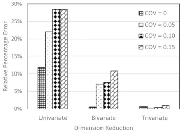
The effect of different number of variate used in the dimension-reduction technique is illustrated in Figs. 4
and 5 for normal and non-normal cases, respectively. For
both cases, it is clear that increasing number of variate will enhance the solution accuracy. However, the influence of COV on different numbers of variate does not have a clear trend. As shown in Fig. 4, relative error (RE) of COV = 0.05 is about 0.3 times that of COV = 0 in the bi-variate case, and RE of COV = 0.05 is about 0.6 times that of COV = 0 in the univariate case. It seems that the COV of random variable has more influence when the number of variate is smaller. However, Fig. 5 displays an opposite trend, RE of COV = 0.05 is more than four times that of COV = 0 in the bi-variate case, while RE of COV = 0.05 is about two times
Table 5 Statistical properties for short column design problem
F (kN) M1 (kN-m) M2 (kN-m) fy (MPa) h (m) b (m)
Mean 2500 250 125 40 μh μb
COV 0.2 0.3 0.3 0.1 0/0.05/0.10/0.15 0/0.05/0.10/0.15
Normal case Normal Normal Normal Normal Normal Normal
Non-normal case Gumbel Gumbel Gumbel Weibull Lognormal Lognormal
Table 6 Comparison of the optimization results for short column design problem
a Solutions from nine points with tri-variate dimension reduction b Equation (33) is used to calculate the error percentage c COV=0.15
Normal case Non-normal case
0 0.05 0.1 0.15 0 0.05 0.1 0.15
Aoues and Chateauneuf [1] 0.1915 0.2024 0.2372 0.3014 0.2014 0.2088 0.2319 0.2717 PSO-4M–3M–2Ma 0.1918 0.2031 0.2394 0.3182 0.2133 0.2209 0.2457 0.2871 Relative errorb 0.2974 0.7110 1.2017 0.9073 0.7338 0.2175 0.3331 0.9724 Ave. runtimec 224.16 837.85 824.86 823.39 274.58 945.87 946.12 963.52 FE per RA 3425 15,809 15,809 15,809 3425 15,809 15,809 15,809 3M (%) 2.6c 2.9c 4M (%) 97.3c 97.1c 0% 5% 10% 15% 20% 25% 30%
Univariate Bivariate Trivariate
Rela tive Perc enta ge Error Dimension Reduction COV = 0 COV = 0.05 COV = 0.10 COV = 0.15
Fig. 4 Relative percentage error of reliability index at optimal point using PSO-4M–3M–2M (normal case)
0% 5% 10% 15% 20% 25% 30%
Univariate Bivariate Trivariate
Rela ve Percentage E rror Dimension Reduc on COV = 0 COV = 0.05 COV = 0.10 COV = 0.15
Fig. 5 Relative percentage error of reliability index at optimal point using PSO-4M–3M–2M non-normal case)
that of COV= 0 in the univariate case. Figure 6 compares the computational speed for the non-normal case with dif-ferent COVs and number of variate. It is seen that the cost of increasing number of variate to enhance the accuracy is around 11 times to that of univariate case.
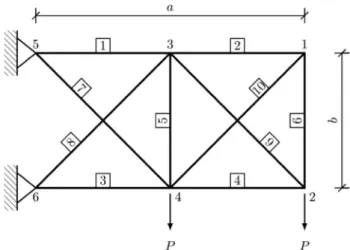
5.3 Ten‑bar truss
To examine the applicability of the proposed PSO-4M–3M–2M on a problem of implicit performance, a clas-sical ten-bar truss problem, adapted from Shayanfar et al. [19], is used. The objective of this ten-bar truss problem is to minimize the total weight of a truss structure, as shown in Fig. 7. The mathematical formulation is given in the fol-lowing equation:
where ρ is the material density (0.1 lb/in.3), A
i is the cross
area of each truss member, Li is the length of each truss
member, G is the performance function, x is vector of ran-dom variable,d = [A1, A2,… , A10]T, G(d, x) = u2− 2 (in.),u2
is the vertical displacement at point 2, as shown in Fig. 7, and βT is the target reliability index (i.e., 3.0). Parameters
of a and b indicated in Fig. 7 are 720 and 360 (in.), respec-tively. As indicated in Eq. (35) and Fig. 7, this ten-bar truss problem has 12 random variables which all follows the nor-mal distribution. The area, A1–10, is both a design variable
and a random variable and the design area is the mean value of the random variable, Ai. The external load, P, has a mean
of 105 lb and the modulus of elasticity, E, has a mean of
107 psi. All 12 random variables have a COV that is equal
to 0.05.
In addition to examine the suitability of the proposed PSO-4M–3M–2M for a problem with implicit function, effects of univariate, bi-variate and tri-variate are also inves-tigated for the dimension reduction. Each dimension-reduc-tion method uses 7, 9, and 11 points for moment estimadimension-reduc-tion. 20 particles in 150 iterations are used in PSO to find the optimal solution. The inertial parameter is linearly decreas-ing from 0.9 to 0.6. c1 and c2 in Eq. (28) are set to be 2.0.
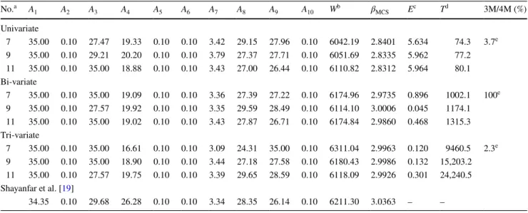
Table 7 displays the optimal area for each truss member using PSO-4M–3M–2M. It is seen that using more number of variate can effectively reduce the relative error percent-ages from approximately 5–0.2%. As expected, the tri-vari-ate case delivers the best accuracy. However, the correspond-ing cost also increases dramatically when the more number of variate is used. Approximately, the cost of using tri-var-iate is 180 times to that of the univartri-var-iate case. On the other hand, increasing number of point in moment estimation does not have a significant effect on the accuracy for all three cases. That is, seven-point estimation is able to precisely provide the moments for the calculation of reliability index. Compared to the literature study [19], it is observed that the proposed method provides a slightly better optimal weight and a better reliability measure compared to the previous study. However, due to the inherent randomness in PSO, the optimal weight of the seven-point estimation in the tri-variate case is slightly higher than other solutions obtained in the current study and the weight indicated in the literature study. It is believed that increasing point of the population or iteration number in PSO can solve this problem.
(35) Min.w= 𝜌 10 ∑ i=1 AiLi, i= 1, 2, … , 10 s.t. Prob[G(d, x)≤ 0] ≤ 𝛷(−𝛽T) 0.10≤ Ai≤ 35.0, 0 200 400 600 800 1,000 1,200
Univariate Bivariate Trivariate
Runtime (sec ) Dimension Reduction COV = 0 COV = 0.05 COV = 0.10 COV = 0.15 1x 4x 11x 1x 2x 4x
Fig. 6 Runtime for short column design problem using PSO-4M– 3M–2M (non-normal case)
5.4 2D‑mathematical problem
To reveal the applicability of the proposed algorithm in solv-ing an RBDO with system reliability, a literature problem from Liao and Ivan [11], and Aoues and Chateauneuf [1] is investigated. The mathematical formulation of the RBDO problem is described in the following equation:
where (36) Min.(d) = (d1+ d2− 8) 2 ∕30 + (d1− d2− 15) 2 ∕120 s.t. Prob.[(g1≤ 0) ∪ (g2≤ 0) ∪ (g3≤ 0) ∪ (g4≤ 0)] ≤ 2.275% 0≤ d ≤ 10, g1(X) = 1 − ((X1− 0.3)2X 2)∕20 g2(X) = 1 − (−0.4226X1+ 0.9063X2) + (0.9063X1+ 0.4226X2− 6)2+ (0.9063X1+ 0.4226X2− 6)3− 0.6(0.9063X1+ 0.4226X2− 6)4) g3(X) = 1 − 80∕(X2 1+ 8X2+ 5) g4(X) = 1 − (X1− X2− 2.5)2∕30 − (X1+ X2+ 4.5)2∕120 X∼ N(d, 0.3) d= [d 1, d2].
It is seen that this is a series system reliability problem with nonlinear constraints. The proposed performance func-tion for this problem based on the descripfunc-tion of “Methods of moments for system reliability” is defined, as in the fol-lowing equation:
Table 8 displays the optimization results. It is seen that the error of the proposed algorithm is slightly larger than that of the previous examples. The simplification of system reliability using Eq. (37) and the simplification of reliabil-ity index using 4M, 3M, or 2M are the potential sources of the error. As discussed in “The proposed RBDO”, within (37)
G(X) = min[g1, g2, g3, g4].
Table 7 Optimal areas for ten-bar truss problem using PSO-4M–3M–2M
a No. of point estimate b Weight
c Relative error (%) d Average running time (s) e 11 point No.a A 1 A2 A3 A4 A5 A6 A7 A8 A9 A10 Wb βMCS Ec Td 3M/4M (%) Univariate 7 35.00 0.10 27.47 19.33 0.10 0.10 3.42 29.15 27.96 0.10 6042.19 2.8401 5.634 74.3 3.7e 9 35.00 0.10 29.21 20.20 0.10 0.10 3.79 27.37 27.71 0.10 6051.69 2.8335 5.962 77.2 11 35.00 0.10 35.00 18.88 0.10 0.10 3.43 27.00 26.44 0.10 6110.82 2.8312 5.964 80.1 Bi-variate 7 35.00 0.10 35.00 19.09 0.10 0.10 3.36 27.39 27.22 0.10 6174.96 2.9735 0.896 1002.1 100e 9 35.00 0.10 27.57 19.92 0.10 0.10 3.35 29.59 28.49 0.10 6114.10 3.0006 0.045 1174.1 11 35.00 0.10 35.00 19.02 0.10 0.10 3.43 27.87 26.71 0.10 6174.84 2.9860 0.468 1315.3 Tri-variate 7 35.00 0.10 35.00 16.61 0.10 0.10 3.09 24.31 35.00 0.10 6311.04 2.9963 0.120 9460.5 2.3e 9 35.00 0.10 35.00 18.90 0.10 0.10 3.44 27.18 27.58 0.10 6180.43 2.9986 0.132 15,203.2 11 35.00 0.10 27.57 19.75 0.10 0.10 3.39 29.65 28.59 0.10 6118.09 2.9926 0.301 24,240.5 Shayanfar et al. [19] 34.35 0.10 29.68 26.28 0.10 0.10 3.34 28.35 26.14 0.10 6211.30 3.0363 – –
Table 8 Solutions of the 2D-mathematical problem
a Eleven point of tri-variate approach is used b Average running time (s)
D1 D2 Cost PFsys PFMCS % Error Tb 3M/4M (%) Liao and Lu [12] 4.401 3.867 1.7461 0.022565 0.022576 0.05 –
the applicable range, the fourth-moment reliability index,
β4M, is expected to provide a more accurate reliability index. However, although this is a general case, it is not always true. It is observed that, in a very few case, β3M provides a better accuracy. Although the proposed RBDO algorithm (PSO-4M–3M–2M) is able to deliver a promising solution for many cases as shown in the numerical examples. More investigation on the moment-based reliability index should be worth for future application.
6 Discussions
RBDO, imposing probabilistic constraints into the optimiza-tion procedure, is one of the approaches to find an optimal design considering the effects of nondeterministic informa-tion. To verify the satisfaction of probabilistic constraints, reliability analysis must be conducted at each design trial, leading to a double-loop procedure which is often a barrier in application. This study investigates accuracy and effi-ciency of the moment-based reliability analysis that is incor-porated with the ε-constrained PSO for RBDO problems. The proposed algorithm is validated using several RBDO problems, and the performance of accuracy, efficiency, and effects of applicable range is discussed below.
The accuracy of the proposed algorithm is evaluated by comparing the solutions from those of the literatures and MCS. Compared to the literatures, the proposed algorithm is able to find better RBDO solutions for all examples, except-ing the solution from Wu et al. [24] in the first example and the solution from Liao and Lu [12] in the fourth example. Compared to the solution of MCS, the relative errors range from 0.008 to 2.63% for four examples if tri-variate method is adopted. The error percentage is often quite small, and the highest error percentage (2.63%) is found from the 2D-math-ematical problem, in which system reliability is considered. The simplification of system reliability using Eq. (37) is considered as the potential source of the error. It is seen that the proposed algorithm often delivers a promising accuracy. In addition, a decreasing trend in relative error is observed when a greater number of variates are used for all examples. From the second example, it is found that the PDF and COV of the random variables only have moderately influence on the error percentage. However, increasing number of point in moment estimation does not have significant effect on the accuracy.
Although a greater number of variates can help enhance the solution accuracy, the function evaluation (FE) signifi-cantly increases in such approach. Taking the first exam-ple for examexam-ple, the FE needed per reliability analysis is only 25 for univariate method, while it is 265 and 993 for bi-variate and tri-variate cases. In terms of the running time, the cost of using tri-variate is 11 and 180 times to
that of univariate case for the short column and the ten-bar truss examples. The ten-ten-bar truss example is used to demonstrate the applicability of the proposed algorithm in a problem with implicit performance functions. That is, finite-element analysis is needed in finding the opti-mal solution, resulting a longer running time. The run-ning time for the ten-bar truss is 9460 s if the suggested approach (i.e., tri-variate with seven-point estimation) is used, which is not quite efficient, but should be still in an acceptable range.
Two applicable ranges of the 4M method are used for comparison. The empirical range (Eq. 23) is built based on allowable relative error (i.e., 2%) among different approaches. Zhao et al. [32] derived a complete expression of the 4M method with different combinations of skew-ness and kurtosis, and investigate the monotonicity of each expression, in which a theoretical applicable range was obtained. Tables 9, 10, and 11 display the results of using empirical and theoretical applicable ranges for the cantile-ver beam, short column, and ten-bar truss problem. For the cantilever beam, it is seen that both equations are able to
Table 9 Comparison of cantilever beam using empirical and theoreti-cal applicable ranges
a The empirical applicable range is used b The theoretical applicable range is used c Nine-point estimation with tri-variate is used
w (in.) t (in.) Area (in.2) MCS Case 1c Equation (23)a 2.4502 3.8805 9.52030 0.00135 Equation (24)b 2.4497 3.8873 9.52140 0.00135 Case 2c Equation (23)a 2.7021 3.4153 9.2285 0.0013498 Equation (24)b 2.7049 3.4119 9.2287 0.0013499
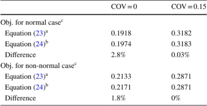
Table 10 Comparison of short column using empirical and
theoreti-cal applicable ranges
a The empirical applicable range is used b The theoretical applicable range is used c Nine-point estimation with tri-variate is used
COV = 0 COV = 0.15
Obj. for normal casec
Equation (23)a 0.1918 0.3182
Equation (24)b 0.1974 0.3183
Difference 2.8% 0.03%
Obj. for non-normal casec
Equation (23)a 0.2133 0.2871
Equation (24)b 0.2171 0.2871
find satisfied solutions that is verified by the MCS. Table 10
displays solution differences between two equations, ranging from 0 to 2.8%, indicating that effects of COV and normal/ non-normal are insignificant. Similarly, for a problem with implicit performance function such as ten-bar truss prob-lem, using empirical or theoretical applicable ranges does not have considerable change. Observed that the applicable ranges indicated in Eqs. 23 and 24 are similar, outcomes of Tables 9, 10, and 11 are reasonable.
7 Conclusions
Based on the results and discussions found here, the pro-posed PSO-4M–3M–2M algorithm is able to deliver a promising design and several important observations are described below.
1. The proposed RBDO algorithm is shown to be a stable method, which is not affected by a problem with non-normal random variables or with nonlinear performance functions.
2. In general, the solutions found by PSO-4M–3M–2M, compared to the literatures, are either more optimal or more approaching to the probabilistic constraint for dif-ferent types of RBDO problems investigated here. This indicates that the moment-based reliability index pro-vides an accurate uncertainty measurement for PSO to find a solution.
3. The accuracy of an RBDO solution is proportional to the number of variate in dimension-reduction method. The drawback of increasing variate number is its computa-tional cost is often higher.
4. Random variable with higher COV generally, but not always decreases the accuracy of the moment-based reli-ability measurement. Using more variate can dramati-cally reduce such error.
5. Increasing number of point in moment estimation is not necessary to enhance the accuracy of reliability analysis. Based on the investigated problem, using seven points appears to be adequate for estimating the reliability index.
References
1. Aoues Y, Chateauneuf A (2010) Benchmark study of numerical methods for reliability-based design optimization. Struct Multi-discip Optim 41(2):277–294. https ://doi.org/10.1007/s0015 8-009-0412-2
2. Du X, Chen W (2004) Sequential optimization and reliability assessment method for efficient probabilistic design. J Mech Des 126(2):225–233. https ://doi.org/10.1115/1.16499 68
3. Eberhart RC, Kennedy J (1995) A new optimizer using particle swarm theory. In: Paper presented at the IEEE international sym-posium on micro machine and human science, Nagoya, Japan, 4–6 October. https ://doi.org/10.1109/mhs.1995.49421 5
4. Fleishman AI (1978) A method for simulating non-normal distri-butions. Psychometrika 43(4):521–532. https ://doi.org/10.1007/ BF022 93811
5. Fourie PC, Groenwold AA (2002) The particle swarm optimi-zation algorithm in size and shape optimioptimi-zation. Struct Multi-discip Optim 23(4):259–267. https ://doi.org/10.1007/s0015 8-002-0188-0
6. Gandomi AH, Yang XS, Alavi AH (2013) Cuckoo search algo-rithm: a metaheuristic approach to solve structural optimization problems. Eng Comput 29(1):17–35. https ://doi.org/10.1007/ s0036 6-012-0308-4
7. Kaveh A, Farhoudi N (2013) A new optimization method: Dolphin echolocation. Adv Eng Softw 59:53–70. https ://doi.org/10.1016/j. adven gsoft .2013.03.004
8. Lee I, Choi KK, Gorsich D (2010) System reliability-based design optimization using the MPP-based dimension reduction method. Struct Multidiscip Optim 41(6):823–839. https ://doi.org/10.1007/ s0015 8-009-0459-0
9. Li Y, Jiang P, Gao L, Shao XY (2013) Sequential optimization and reliability assessment for multidisciplinary design optimization under hybrid uncertainty of randomness and fuzziness. J Eng Des 24(5):363–382. https ://doi.org/10.1080/09544 828.2012.75399 5
10. Liao KW, Ha C (2008) Application of reliability-based optimi-zation to earth-moving machine: hydraulic cylinder components design process. Struct Multidiscip Optim 36(5):523–536. https :// doi.org/10.1007/s0015 8-007-0187-2
11. Liao KW, Ivan G (2014) A single loop reliability-based design optimization using EPM and MPP-based PSO. Latin Am J Solids Struct 11(5):826–847. https ://doi.org/10.1590/S1679 -78252 01400 05000 06
12. Liao KW, Lu HJ (2012) A stability investigation of a simula-tion- and reliability-based optimization. Struct Multidiscip Optim 46(5):761–781. https ://doi.org/10.1007/s0015 8-012-0793-5
13. Liu X, Zhang Z (2014) A hybrid reliability approach for structure optimization based on probability and ellipsoidal convex mod-els. J Eng Des 25(4–6):238–258. https ://doi.org/10.1080/09544 828.2014.96106 0
14. Mansour R, Olsson M (2016) Response surface single loop reliability-based design optimization with higher-order reliabil-ity assessment. Struct Multidiscip Optim 54:63–79. https ://doi. org/10.1007/s0015 8-015-1386-x
Table 11 Comparison of ten-bar truss using empirical and theoretical applicable ranges
a The empirical applicable range is used b The theoretical applicable range is used
Case A1 A2 A3 A4 A5 A6 A7 A8 A9 A10 Wb Diff.
Tri-variate with 11 points
Aa 35.00 0.10 27.57 19.75 0.10 0.10 3.39 29.65 28.59 0.10 6118.09 0.7% Bb 35.00 0.10 27.99 20.14 0.10 0.10 3.36 28.89 28.83 0.10 6119.50
15. Qu X, Haftka RT (2004) Reliability-based design optimization using probabilistic sufficiency factor. Struct Multidiscip Optim 27(5):314–325. https ://doi.org/10.1007/s0015 8-004-0390-3
16. Ramu P, Qu X, Youn BD, Haftka RT (2006) Inverse reliability measures and reliability-based design optimization. Int J Reliab Saf 1:187–205. https ://doi.org/10.1504/IJRS.2006.01069 7
17. Raza MA, Liang W (2012) Uncertainty-based computational robust design optimization of dual-thrust propulsion sys-tem. J Eng Des 23(8):618–634. https ://doi.org/10.1080/09544 828.2011.63601 125
18. Shan SQ, Wang GG (2008) Reliable design space and complete single-loop reliability-based design optimization. Reliab Eng Syst Saf 93(8):1218–1230. https ://doi.org/10.1016/j.ress.2007.07.006
19. Shayanfar M, Abbasnia R, Khodam A (2014) Development of a GA-based method for reliability-based optimization of structures with discrete and continuous design variables using OpenSees and Tcl. Finite Elem Anal Des 90:61–73. https ://doi.org/10.1016/j. finel .2014.06.010
20. Takahama T, Sakai S, Iwane N (2005) Constrained optimization by the ε constrained hybrid algorithm of particle swarm opti-mization and genetic algorithm. In: Paper presented at the 18th Australasian joint conference on artificial intelligence, Sydney, Australia, 5–9 December. https ://doi.org/10.1007/11589 990_41
21. Tichy M (1994) First-order third-moment reliability method. Struct Saf 16(3):189–200. https ://doi.org/10.1016/0167-4730(94)00021 -H
22. Venter G, Sobieszczanski-Sobieski J (2004) Multidisciplinary optimization of a transport aircraft wing using particle swarm optimization. Struct Multidiscip Optim 26(1):121–131. https :// doi.org/10.1007/s0015 8-003-0318-3
23. Wang J, Lu ZH, Saito T, Zhang XG, Zhao YG (2017) A sim-ple third-moment reliability index. J Asian Archit Build Eng 16(1):171–178. https ://doi.org/10.3130/jaabe .16.171
24. Wu YT, Shin Y, Sues R, Cesare M (2001) Safety-factor based approach for probability-based design optimization. In: Paper presented at the 42rd AIAA/ASME/ASCE/AHS/ASC structures,
structural dynamics, and materials conference: AIAA-2001–1522, Seattle, WA, 16–19 Apr. https ://doi.org/10.2514/6.2001-1522
25. Xu H, Rahman S (2004) A generalized dimension-reduction method for multidimensional integration in stochastic mechanics. Int J Numer Meth Eng 61(12):1992–2019. https ://doi.org/10.1002/ nme.1135
26. Yi P, Zhu Z, Gong J (2016) An approximate sequential optimiza-tion and reliability assessment method for reliability-based design optimization. Struct Multidiscip Optim 54(6):1367–1378. https :// doi.org/10.1007/s0015 8-016-1478-2
27. Zhao YG, Jin D, Saito T, Lu ZH (2014) System reliability assess-ment using dimension reduction integration. J Jpn Ind Manag Assoc 64(4):562–569. https ://doi.org/10.11221 /jima.64.562
28. Zhao YG, Ono T (2000) Third-Moment standardization for struc-tural reliability analysis. J Struct Eng 126(6):724–732. https ://doi. org/10.1061/(ASCE)0733-9445(2000)126:6(724)
29. Zhao YG, Ono T (2001) Moment methods for structural reli-ability. Struct Saf 23(1):47–75. https ://doi.org/10.1016/S0167 -4730(00)00027 -8
30. Zhao YG, Lu ZH (2007) Fourth-Moment standardization for struc-tural reliability assessment. J Struct Eng 133(7):916–924. https :// doi.org/10.1061/(ASCE)0733-9445(2007)133:7(916)
31. Zhao YG, Lu ZH, Ono T (2006) Estimating load and resistance factors without using distributions of random variables. J Asian Archit Build Eng 5(2):325–332. https ://doi.org/10.3130/jaabe .5.325
32. Zhao YG, Zhang XY, Lu ZH (2018) Complete monotonic expres-sion of the fourth-moment normal transformation for structural reliability. Comput Struct 196:186–199. https ://doi.org/10.1016/j. comps truc.2017.11.006
Publisher’s Note Springer Nature remains neutral with regard to jurisdictional claims in published maps and institutional affiliations.