機場地面路徑規劃及防撞系統研究

行政院國家科學委員會專題研究計畫 成果報告

機場地面路徑規劃及防撞系統研究

計畫類別： 個別型計畫

計畫編號： NSC91-2212-E-002-061-

執行期間： 91 年 08 月 01 日至 92 年 07 月 31 日

執行單位： 國立臺灣大學應用力學研究所

計畫主持人： 王立昇

報告類型： 精簡報告

處理方式： 本計畫可公開查詢

中 華 民 國 92 年 10 月 14 日

機場地面路徑規劃及防撞系統研究

Airport Surface Motion Planning and Collision Avoidance System

計畫主持人: 王立昇

執行單位: 台灣大學應用力學研究所

計畫編號: NSC 91-2212-E-002-061

執行期間: 91 年 8 月 1 日至 92 年 7 月 31 日

Abstract − In this report1

, the methodology of generating an optimal trajectory on a complex surface for a specific vehicle is proposed. The possible paths are constrained by the limitations on the terrain and the capability of the vehicle. To deal with these constraints, the notions of forbidden point, forbidden direction, and forbidden path are introduced. After certain constants are specified, the method of dynamic programming is then invoked to find the optimal solution. If the target is beyond the maximal range of the vehicle, appropriate service stations are selected by using the auction algorithm. To speed up the computation process, the ideas of bi-spiral scheme and instant update are employed. With all the techniques at hand, numerical results show that the proposed method can generate the desired trajectory efficiently. The method may be used to solve the path planning problems for various vehicles on the surface of an airport.

1. Introduction

For a vehicle moving on a complex terrain, its capability restricts the possible paths that it can follow. A jeep can climb a steeper slope than a passenger car, while a mobile robot may be able to climb even steeper slope. Different wear on the tire leads to different limit on the angle of turn. How to accommodate these constraints on the generation of optimal trajectory on a complex terrain is the main theme of this paper.

The constraints on the path may come from either the topology of the terrain or the vehicle itself. On the terrain, there may be some hazardous region or congested area that the vehicle cannot enter. There may be some service stations that the vehicle may need to pass. On the part of the vehicle, sharp turns may not be able to trace and it is preferred to move on a flat path rather than a slope. As a result, the classical algorithm of finding the shortest path needs to be modified. For the shortest-path problem, various techniques have been used to find the optimal solution. These include the Label correcting method [1], D'ijkstra's method [3], method of dynamic programming [6][7][8][9], and the auction algorithm [2]. If the dynamics of the vehicle is taken into consideration, various scheme such as the

1

Part of this report has been presented in IEEE Conference on Robotics and Automation, September 2003.

Hamilton-Jacobi’s method can be adopted, as reviewed in [10]. However, if the complicated dynamical behavior is considered through certain constraints, for the corresponding path planning problems in which other characteristics, in addition to the length of the path, must be considered, the method of dynamic programming provides the most flexible platform based on the principle of optimality. The idea of dynamic programming has been used in [5] to find the optimal path of a vehicle on a terrain by including the consideration of forbidden region and the slope. In this paper, similar idea is adopted to find the optimal solution by considering more realistic limitations and the capability of the vehicle.

In particular, the notions of forbidden directions and forbidden paths are introduced in this paper. The limitations of rate of climb, minimal angle of turn, and maximal distance of travel are incorporated into the algorithm. Depending on the slope of the path, the scaled distance is used to perform the optimization process, so that flatter paths are preferred. If the length of the optimal path exceeds a certain bound, the vehicle needs to pass through some service stations. For this problem, we first transform it to a classical salesman problem and then use the auction algorithm to select the suitable service stations. Moreover, to enhance the computational speed, the notion of bi-spiral scheme is introduced and the technique of instant update is applied. From the numerical results shown is this paper, the methodology proposed here can indeed generate an optimal trajectory that meets all the above-mentioned requirements.

The rest of this paper is organized as follows. In Section 2, the underlying problem of path planning on a complex terrain is described in more detail. Section 3 presents the setup for realizing those constraints and the process of incorporating them into the method of dynamic programming. The algorithm for the selection of service stations and the bi-spiral scheme are also discussed. Numerical results are shown in Section 4, which shows the effectiveness of the proposed method. Hardware experiments for the motion planning and control of a model car are described in Section 5. Finally, some concluding remarks are given in Section 6.

2. Problem Description

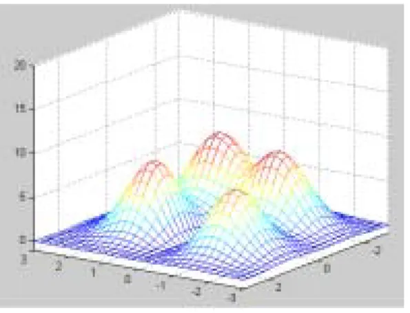
Consider a complex terrain, such as in Figure 1, consisting of geometric points with

each position being specified by three components

(x,y,z)

, with the corresponding

axes being pointing toward the east, the north, and upward, respectively. The

horizontal plane on which the terrain resides may be divided into small rectangles

with a matrix of grid points

(xi,yj), i=1,...,l; j=1,...,n,

which are equally spaced

with distance

a

, cf. Fig. 1. The point on the terrain corresponding to node

( ji, )

is

represented by

P( ji, )

and the height at that point is given by

z( ji, )

. There may be

some regions on the terrain that the vehicle is prohibited to pass, such as a hazardous

area, a lake or a building, which is identified as the set

Ω

. Moreover, it may be

necessary for the vehicle to stop somewhere during the travel for service stations,

such as gas stations. The locations of the service stations on the terrain are denoted by

nodes

g ,...,₁ g_N

.

Fig. 1 complex terrain

The problem is to seek efficiently the optimal trajectory from a starting node

)

, (i_s j_s

s=

to a target node

t=(i_t,j_t)

without entering

Ω

such that the designated

vehicle is able to follow. Different types of vehicles, such as a passenger car, a jeep, or

a truck, have different capabilities, such that their motions are subject to various

constrains. First, the initial direction of the path must be compatible with the heading

of the vehicle at the node

s

. There may be some other nodes for which the direction

of passing is limited. Secondly, the vehicle may not be able to move on a steep slope.

This renders the limitation on the rate of climb of the trajectory. Thirdly, the vehicle

may not be able to make sharp turns, and hence the radius of curvature of the path is

constrained. Moreover, the maximum distance of travel may require the vehicle to

stop at some service station if the destination is too far to reach with one gas tank. In

addition, flat paths are preferred than the paths with steeper slope to save the energy.

Other constraints may be imposed on the trajectory of motion. Those listed above

shall be accommodated in the generation of the optimal path as discussed in the next

section.

3. The algorithm

as discussed in [5]. First, we define the forbidden function

F

as

   ∈Ω = otherwise, , 1 , ) , ( if , 0 ) , (i j i j F

(1)

in which

Ω

is defined in the previous section. In order to describe the move from

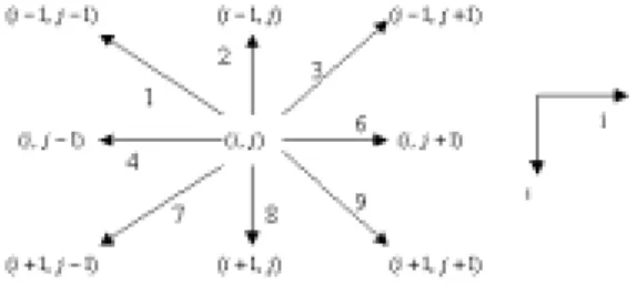
one node to its neighbours, the virtual move

m

is defined to be in the set of

} 9 , 8 , 7 , 6 , 4 , 3 , 2 , 1 { = + M

such that

m=1

represents the move from

( ji, )

to

(i−1,j−1)

, cf. Fig. 2, in which the

meanings of the other values of

m

are also given. Moreover, we use

m=5

to denote

the degenerate virtual move which refers to the move from one node to itself.

Fig. 2 Virtual Moves

For the virtual move

m

, the maps

ϕ,φ

are defined such that

(ϕ(i,m),φ(j,m))

is the

destined node from

( ji, )

via

m

. The distance and the slope of the virtual move

m

from

( ji, )

are then computed from, respectively

2 / 1 2 2 2 2 2

]

))

,

(

))

,

(

),

,

(

(

(

)

)

,

(

(

)

)

,

(

(

[

)

,

,

(

j

i

z

m

j

m

i

z

j

m

j

a

i

m

i

a

m

j

i

dist

−

+

−

+

−

=

φ

ϕ

φ

ϕ

)

)

)

,

(

(

)

)

,

(

(

)

,

(

))

,

(

),

,

(

(

(

tan

)

,

,

(

2 2 1

j

m

j

i

m

i

a

j

i

z

m

j

m

i

z

m

j

i

−

+

−

−

=

−

φ

ϕ

φ

ϕ

α

Let the limitation on the rate of climb of the trajectory be represented by the maximal

upward slope

α

and maximal downward slope

α

, which are determined by the

vehicle. To realize the forbidden region, the limitation on the rate of climb, and the

preference of the flat paths, the scaled distance function for the virtual move

m

from

) , ( ji

is defined as

(

)

              ⋅ +           < > = = > − = > − = = otherwise , ) , , ( ) 1 | ) , , ( | ( ) , , ( or ) , , ( or 0 ) , ( ), , ( or 0 ) , ( or or 1 ) , ( or or 1 ) , ( if , 1 ) , , ( 0 i j m dist i j m w m j i m j i m j m i F j i F n m j l m i -m j i D α α α α α φ ϕ φ ϕ

(2)

in which the scale factor

w

₀

is specified according to the preference on the slope of

the path. It is seen that if the slope of the virtual move

m

is too large, the distance of

the move is set to –1, which indicates that the corresponding virtual move is

prohibited. Moreover, by adjusting the scale factor, the preference of the flatter paths

can be realized.

As discussed in the previous section, the directions of passing through some nodes are limited. The set of such nodes, denoted by b∈B, contains at least the starting node

s

. Since the direction of entering b and that of leaving b may have different constraints, we expand the set of virtual moves to include their reversals, denoted by

} 9 , 8 , 7 , 6 , 4 , 3 , 2 , 1 {− − − − − − − − = − M ,

cf. Fig. 2. The maps ϕ and

φ

are defined accordingly for

m

<

0

. The forbidden directions of passing through the node

b

are then given by a set A(ib,jb)⊂M+∪M−, in which the positive value refers to leaving and negative value refers to entering. If the direction is not allowed, the corresponding virtual move must be prohibited, and the scaled distance function is updated according to the following rule 1 ) 10 ), , ( ), , ( ( 0 1 ) , , ( 0 ), , ( − = + < − = > ∈ m m j m i D then m if m j i D then m if j i A m for b b b b b b φ ϕ (3)

Note that for entering forbidden directions, the corresponding virtual moves from (ϕ(ib,m),φ(jb,m))

is set to be prohibited.

assumed to be composed of two consecutive line segments between nodes. Consider two consecutive virtual moves , , m m such that ) ~ , ~ ( ) ˆ , ˆ ( ) , ( , j i j i j i m m → → .

The angle of turn is then given by

)

~

,

~

(

)

ˆ

,

ˆ

(

,

)

ˆ

,

ˆ

(

)

,

(

)

,

,

,

(

,

j

i

P

j

i

P

j

i

P

j

i

P

m

m

j

i

∠

=

β

i.e. the angle intersected by the segments P(i,j)P(iˆ,ˆj) and P(iˆ,ˆj)P(~i,~j). The constraint of turning may be then realized by requiring

0 , ) , , , ( β β i j m m >

where

β

₀ is some constant determined by the type of the vehicle. The path is forbidden if the previous condition is violated.

With the above setup, we now ready to invoke the method of dynamic programming by a recursive process. Since the direction of move is essential in our consideration, we define the total cost starting from ( ji, ) in the direction of m within

k

moves by C(k,i,j,m). At the step k=0, the cost function is initialized to be 0 at the node

t

, and –1 at all other nodes for all virtual moves. As the algorithm proceeds, the value of the cost function is updated according to the following procedure. At step

k

, at the node ( ji, ) in the direction m such that D(i,j,m)≠−1, we first construct the set of admissible second moves as

}. ) , , , ( , 1 ) ), , ( ), , ( , ( , 1 ) ), , ( ), , ( ( : { ) , , , ( 0 , , , , β β φ ϕ φ ϕ > − ≠ − ≠ ∈ = + m m j i m m j m i k C m m j m i D M m m j i k S (4)

(

)

(

)

(

)

(

)

(

)

(

)

(

)

5 ) , , , 1 ( ), , , , ( ) , , , 1 ( ) , , , 1 ( ) , , , ( ' ), , ( ), , ( , ) , , ( min arg , , , 1 ' ), , ( ), , ( , ) , , ( min , , , 1 1 , , , 1 ) , , , ( ) , , , ( ' ) , , , ( ' = + = + + ≤ + = + + = + − = + ∈ ∈ m j i k m j i k C m j i k C then m j i k C m j i k C if m m i m i k C m j i D m j i k m m i m i k C m j i D m j i k C else m j i k C set empty is m j i k S if m j i k S m m j i k S m γ φ ϕ γ φ ϕ (5)

It is noted that in the second part of the previous procedure, if the above minimization process yields a cost for step k+1 is greater than or equal to that for step

k

, further virtual move is not appropriate, and hence degenerate move occurs.

The above iteration proceeds until all the virtual moves become degenerate, which is equivalent to the condition, m j i m j i k C m j i k C( +1,, , )= ( ,, , ), ∀, , .

At the final stage, say step k , the minimal cost of the optimal path starting from any node ( ji, ) to the target t in any direction m is obtained. We may then start with

s

and utilize the map γ to trace back the optimal path as follow:

(

)

{

}

( )

( )

) , , , ( , , 5 ) , , , ( 1 0 , , , min arg * * * * * * * * * ∗ ∗ ∗ ∗ ∗ ∗ ∈ ∗ − ← ← ← ≠ − − = = = = ₊ m j i p k m m j j m i i then m j i q k if k to q for j j i i m j i k C m s s s s M m γ φ ϕ γ (6)

The established path shall then be the optimal one satisfying the constraints discussed in Section 2 except the maximal distance of travel.

To meet the requirement of maximal range R_max for a specific vehicle, we first compute the length of the optimal path found in the above process, say R_opt. If

max

R

Ropt > , then we need to find suitable

intermediate service stations. The strategy is to seek the optimal path for each pair of nodes in the set

} , ,..., ,

{s g1 gN t . Deleting those paths with length greater than Rmax, the problem becomes the classical

obtain the optimal solution. Here we adopt the auction algorithm as discussed in [2] for its flexibility in dealing with the changes of distance functions.

Fig. 3 Salesman Problem and Auction Algorithm

The above process may be very time-consuming if the terrain is large. In order to

speed up the computation process, we adopt the bi-spiral scheme in the update process

of the cost function. The sequence of nodes visited in each step k to apply the process

（5） starts with a neighbouring node of the target t, then proceeds spirally outward.

Once all the nodes are visited, the update process reverses its direction to spirally

inward return to the target. This sequence can significantly reduce the total number of

steps, especially when the desired path is curved back and forth. Moreover, in the

minimization process of （5）, we could use the updated

C(k+1,ϕ(i,m),φ(j,m),m,)

,

instead of

( , (, ), ( , ), ,) m m j m i k

C ϕ φ

if the node

(

ϕ

(i,m),

φ

(j,m))

has been visited at step

1

+

k

. This idea of instant update is similar to that of Gauss-Siedel method [4] in

solving a set of algebraic equations, and can enhance the efficiency of the algorithm

prominently.

4. Numerical Result

For the example of complex terrain shown in Fig. 1, we are now ready to apply the

algorithm developed in Section 3 to find the optimal trajectory satisfying the

constraints. First, we divide the horizontal plane into 31*31 grid nodes with grid

length

a=5

(meter), and consider the case that

R_max =∞

, i.e. the vehicle can move to

any point on the terrain without service. Let the capability of the vehicle and the

preference of slope impose the constraint on the possible path through the following

constants：

7 . 0 = α

,

α=−0.8

,

0 0 =120 β

,

w₀=4.0

.

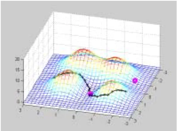
Incorporating these constants in the algorithm, the optimal trajectory from the node

) 21 , 5 ( =

s

to the target

t=(26, 18)

is then obtained as shown in Fig. 4. The

trajectory winds around the hills to reach the target.

If the constraint of maximal range is set as

R_max=250

(meter), the vehicle cannot

reach the target without service. The strategy outlined in Section 4 using the auction

algorithm is then followed to find suitable intermediate service stations. The result is

shown in Fig. 5, in which the service stations are marked by big circles. For the same

set of the starting node and the target node, another trajectory is chosen to pass by a

service station. From these examples, it is seen that the methodology proposed in this

paper can indeed give rise to an optimal trajectory satisfying all the constraints

described before.

Fig. 4. Optimal Trajectory with Infinite Maximum Range

Fig. 5. Optimal Trajectory with Limited Maximum Range

5. Hardware experiments

To check the effectiveness of the proposed method, the methodology of finding an

optimal path and designing a controller for a model car is developed. The model car

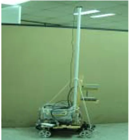
is re-configured, cf. Figure 6, so that various sensors, such as GPS receiver, electronic

compass, and data links can be put on the vehicle, which is controlled by the base

station. With differential GPS carrier phase algorithm, the position of the vehicle

can be determined with the accuracy about 10 centi-meters. The positioning

information and the heading information from the compass are then fed into the

path-planning algorithm. With the destined position and the desired orientation

being specified, the method discussed before is used to generate an optimal path. A

fuzzy controller is then used to control the vehicle move on the designed path. An

experimental result is shown in Fig. 7.

The vehicle was set to move on a flat surface, which was grided into square

elements. The path generated by the above-mentioned dynamic programming

algorithm is further smoothed by using the B-spline method, as shown by the solid

line in Figure 7. The result of the controlled motion of the vehicle is shown as the

dotted line in Figure 7. The error is about 1 meter. Through hardware experiments, it

is demonstrated that the proposed methodology can indeed generate a path suitable for

a specific vehicle.

Fig. 6. Re-configured Model Car

6. Conclusion

This paper presents a methodology to generate an optimal path on a complex 3-D

terrain that a specific vehicle is safe and capable to follow. Numerical results show

that the method is effective and efficient. The algorithm can be used for a variety of

vehicles, such as a passenger car, a truck, or a mobile robot, by choosing the

appropriate constants in the algorithm. In addition to those constraints considered here,

there may be many other limitations or preference to be included. The effect of the

roughness of the terrain on the selection of path is an example. Hardware experiments

of a model car moving on a surface were performed, which showed the effectiveness

of the proposed method.

6. References

[1] Bertsekas, D.P., Dynamic Programming and Optimal Control, Athena Scientific, 1995.

[2] Bertsekas, D.P., “An Auction Algorithm for Shortest Paths,’’ SIAM J. on Optimization, vol. 1, pp.425-447, 1991.

[3] Dijkstra, E.W., “A Note on Two Problems in Connection with Graphs,” Numer. Math., vol. 1, pp. 269-271, 1959.

[4] Gerald, C.F., Wheatley, P.O., Applied Numerical Analysis, Addison-Wesley Publishing Company, 1994.

[5] Kwok, K.S., Driessen, B.J., “Path Planning for Complex Terrain Navigation Via Dynamic Programming,” Proc. of American Control Conference, S.D., Cal., pp. 2941-2944, 1999.

[6] Lam, K.P., Tong, C.W., “Connectionist Network for Dynamic Programming Problems”, IEE

Proc.-Comput. Digit. Tech., vol. 144, No. 3, pp. 163-167, 1997.

[7] Larson, R.E., Casti, J.L., Principles of Dynamic Programming - PartⅡ Advanced Theory and

applications, Marcel Dekker Inc., 1982.

[8] Lewis, F.L., Syrmos, V.L., Optimal Control, John Wiley & Sons, 1995.

[9] Ravindran, A., Phillips, D.T., Solberg, J.J., Operations Research - Principles and Practice, John Wiley & Sons, 1987.

[10] Tsitsiklis, J.N., “Efficient Algorithms for Globally Optimal Trajectories,” IEEE Trans. on Aumatic