O2TC：利用二進制優點的高品質、低複雜度二進制材質壓縮法

國

立

交

通

大

學

資訊學院 資訊學程

碩

士

論

文

O2TC：利用二進制優點的高品質、低複雜度二進制材

質壓縮法

O2TC：Exploiting Binary Virtues with

High-Quality, Low Complexity Order-of-2 Texture

Compression

研 究 生：柯天人

指導教授：鍾崇斌 教授

O2TC：利用二進制優點的高品質、低複雜度二進制材質壓縮法

O2TC：Exploiting Binary Virtues with High-Quality, Low

Complexity Order-of-2 Texture Compression

研 究 生：柯天人 Student：Tien-Jen Ke

指導教授：鍾崇斌 Advisor：Chung-Ping Chung

國 立 交 通 大 學

資訊學院 資訊學程

碩 士 論 文

A Thesis

Submitted to College of Computer Science National Chiao Tung University in partial Fulfillment of the Requirements

for the Degree of Master of Science

in

Computer Science December 2009

Hsinchu, Taiwan, Republic of China

O2TC：利用二進制優點的高品質、低複雜度二進制材質壓縮法

學生：柯天人 指導教授：

鍾崇斌

國立交通大學 資訊學院 資訊學程碩士班

摘要

對於儲存空間或是傳輸頻寬有限的裝置材質壓縮是需要的。雖然有損耗的壓縮是有效 的，但是解壓縮後的材質品質是一個問題。我們提出一個可以達成壓縮率高、解碼簡單 而且解碼後的品質高的二進制材質壓縮法—O2TC (Order of 2 Texture Compression)。 O2TC 試著利用二進制系統的優點。他的特點包含:對用來表示的基本顏色做明智的選擇 與編碼、簡單而且可平行接收方塊材元。我們使用一對基本顏色或是一個基本色與一個 差值，加上簡單快速的二進制內插與外插計算出用來表示的顏色，使用平移運算而不需 要使用乘法或是除法。使用隱藏位元來最小化因截斷所造成的最大可能誤差。我們也進 一步減少壓縮/解壓縮的運算誤差。並且透明分量也可以使用一樣的方法。跟著名的 S3TC 的 DXT5 方法比較，我們有更簡單的解壓縮方式與更好的解壓縮後影像品質，在有透明 分量的材質上，O2TC RGB888, 8-color, 與 Plain64-64 options 方法分別領先了 0.37, 2.80 and 0.15 dB。更簡單的解壓縮方法代表相同時間內可以產生更多的材元顏色。

O2TC：Exploiting Binary Virtues with High-Quality, Low Complexity

Order-of-2 Texture Compression

Student：Tien-Jen Ke Advisor：Chung-Ping Chung

Degree Program of Computer Science

Nation Chiao Tung University

ABSTRACT

Texture compression is necessary for limited storage and low bandwidth devices. While lossy compressions are effective, quality of texture after recovery becomes an issue. We propose an order-of-two texture compression method—O2TC (Order of 2 Texture

Compression) to achieve high compression rate, easy decompression, and high quality after decompression. O2TC tries to exploit virtues in binary system. Its attributes include: judicious selection and coding of representative base colors, and simple and parallelizable retrieval of block of texels. We use either a pair of base colors or a base colors and a difference, and simple and fast binary calculations—without *, ÷ or approximation—to inter/extrapolate them into representative colors. Truncation error upper bound is also minimized with implicit color bits. With 2’s complement arithmetic, we further reduce the compression/decompression error. And alpha channel can be treated the same. Compared with renowned S3TC’s DXT5, our method has much simplified decompression with better texture quality—0.37, 2.80 and 0.15 dB better on average with O2TC RGB888, 8-color, and Plain64-64 options, respectively, on popular alpha maps.

誌謝

首先感謝我的指導老師 鍾崇斌教授，在這兩年來的辛勤教導讓我可以順利完成此 論文，並且可以順利通過口試。同時感謝我的口試委員洪士灝教授、單智君教授以及邱 日清教授，由於他們的指導與建議，讓這篇論文更加完整與確實。 另外，感謝指導我的楊惠親學姐，學姊在論文上給我許多寶貴的意見。同時也要感 謝實驗室的同學之傑、秀青、浤偉與東霖，大家在每次討論上都給予許多的建議，感謝 大家這兩年的相互鼓勵讓我研究生的生活非常順利與快樂 也要感謝我的老婆，淑鈴。在忙著做研究時可以體諒我並且支持我，讓我無後顧之 憂，也讓我可以安心順利的完成學業。最後也感謝公司的上司 Andrew 這兩年的支持與 工作上的安排讓我可以順利完成學業。 謹向所有支持我，勉勵我的師長與親友，獻上最誠摯的祝福，感謝你們。 柯天人 2009. 11. 19

Table of Contents

摘要………...………...…….-I- ABSTRACT………..………..………-II- 誌謝………...…….-III- Table of Contents………...…………-IV- List of Figures………...………...………….-VII- List of Tables……….………...………….-IX- Chapter 1 Introduction………...………-1-

1.1 GPU and Programmable Graphics Render Pipeline………...-1-

1.1.1 Vertex Processing……….………...-3-

1.1.2 Triangle Setup and Rasterization……….………-3-

1.1.3 Pixel Processing………..-4-

1.1.4 Depth Processing……….………-4-

1.2 Texture Mapping and Texture Filtering………..…-5-

1.2.1 Texture Mapping……….-5- 1.2.2 Texture Filtering………..-6- 1.2.3 Texture Compression……….……..-8- 1.3 Motivation………..………-9- 1.4 Objective……….….-10- 1.5 Thesis Organization…..………..……..-11- Chapter 2 Background………...………….-12-

2.1 Block Truncation Coding……….…………-12-

2.2 Color Cell Compression………..…….-13-

2.3 S3 Texture Compression………..……….-13-

2.4 iPACKMAN……….………...-14-

Chapter 3 Design………..………….-17- 3.1 Basic Ideas……….……….……….…-17- 3.2 Inter/Extrapolation Mode……….………-18- 3.2.1 Bits Layout………-20- 3.2.2 Errors computation………....……-21- 3.2.3 Texture decompression………..……-22- 3.2.4 Parallel Decompression……….………-25-

3.2.5 Discussion of inter/extrapolation mode……….-26-

3.3 Advanced Differential mode……….-27-

3.3.1 Bits Layout………-28-

3.3.2 Encode and errors comput ation……….-30-

3.3.3 Texture decompression……….…….-31-

3.3.4 Parallel Decompression……….………-33-

3.3.5 Discussion of advanced differential mode………-34-

3.4 Texture encode………..………-35-

3.5 Texture with Alpha channel………..………-36-

3.5.1 Bits layout……….………….-38-

3.6 Overall Design………..-39-

Chapter 4 Experiment Results………...………….-41-

4.1 Simulation Environment………..………….-41-

4.2 Quality Measure………..……….-41-

4.3 Software Simulation Results………..…..-42-

4.3.1 Various padding methods………..-42-

4.3.2 Various code words format……….……...-43-

4.3.3 Various 64 bits methods……….………-44-

4.3.4 Various 128 bits methods with alpha channel………...-45-

4.4 Timing and Circuit Complexity Analyses………..……..-46-

5.1 Evaluations and Discussion………..………-48-

5.2 Conclusion and Future Work………..…..-49-

References………..-50-

List of Figures

Figure 1 Programmable graphics render pipeline……….-2-

Figure 2 Triangle rasterization………..-4-

Figure 3 A texture, its width and height are all eight………-5-

Figure 4 Concept of texture mapping………...-6-

Figure 5 Left: when minification occurs the fragment footprint covers many texels, Right: when magnification occurs, few or only one texel is covered by the footprint………....-7-

Figure 6 Concept of trilinear and mip-map texture………..…-8-

Figure 7 The texture unit with texture compression technique………-9-

Figure 8 The concept of BTC……….-12-

Figure 9 The concept of CCC……….-13-

Figure 10 The concept of S3TC………..-14-

Figure 11 The decompressor design of iPACKMAN……….-15-

Figure 12 Stored color of S3TC……….-19-

Figure 13 Stored colors of basic Inter/Extrapolation mode of O2TC………-19-

Figure 14 Bits layout of compression in Inter/Extrapolation mode of O2TC………….…..-20-

Figure 15 Bits stored of red, green and blue of one base color……….….-21-

Figure 16 The range that padding b100 presented……….…-22-

Figure 17 This diagram shows a possible decompressor of basic Inter/Extrapolation mode of O2TC……….…….-23-

Figure 18 O2TC option1 parallel texture retrieval circuit, with its 2-color generator show in the lower part………..-26-

Figure 19 Stored colors of advanced differential mode of O2TC………..-27-

Figure 20 Bits stored of red, green and blue of Option2 of O2TC……….…………-29-

Figure 21 Bits layout of compression in Option2 of O2TC………...-29-

Figure 23 The range that padding b10 presented……….………...-31-

Figure 24 This diagram shows a possible decompressor of Option2 of O2TC………..……-32-

Figure 25 O2TC Option2 parallel texture retrieval circuit, with its 3-color generator show in the lower part……….…………-34-

Figure 26 Base colors selection flowchart in texture block compression…………..………-36-

Figure 27 Alpha channel compression/decompression of DXT5……….…….-37-

Figure 28 Alpha channel compression/decompression of Option1 of O2TC………-37-

Figure 29 Alpha channel compression/decompression of Option2 of O2TC………-38-

Figure 30 Option1 of O2TC with alpha – a plain 64-64 format……….…………-39-

Figure 31 O2TC Option1, the 8-color format with alpha………...-39-

Figure 32 O2TC Option2, the 8-color format with alpha……….……..-39-

Figure 33 Overall design of O2TC……….-40-

Figure 34 PSNR results of various methods………..…………-44-

List of Tables

Table 1 Input, output and operation of each stage………...-2-

Table 2 The true table of control signals and results of computation in basic inter/extrapolation mode of O2TC………....-24-

Table 3 The true table of control signals and results of computation in advanced differential mode of O2TC………-32-

Table 4 Quality comparison of padding variations……….-42-

Table 5 Quality comparison of O2TC Option2 variations………..…-43-

Table 6 Quality comparison of O2TC Option2 variations………..…-44-

Table 7 Quality comparison of DXT5_Theo and various O2TC………..….-45-

Table 8 Timing and circuit complexity of various one-texel-at-a-time retrieval methods…- 46- Table 9 Quality, hardware, timing comparison of Option1 and Option2 of O2TC and S3TC………..…… -48-

Chapter 1 Introduction

1.1 GPU and Programmable Graphics Render

Pipeline

In the nowadays, Graphic processing unit (GPU) is an important of field of application specific processor. It targets on graphics rendering, which display the two-dimensional (2D) viewing of three-dimensional (3D) space. The modern GPU becomes more complex due to users’ increasing demands for 3D scene realism improvement [1].

Programmable graphics pipeline is the most popular solution for the requirements of both performance and flexibility in computer graphics nowadays. With the rapidly development of computer graphics, such as 3D games, virtual realities and digital lives, the requirements of computer graphics in effects and performance become higher [2]. To achieve all kinds of users’ requirements, the programmable graphics pipeline is the best solution builds into graphics hardware and many complicated function units have been builds in. The programmable graphics pipeline has new graphics processing units: vertex shader unit and pixel shader unit, which is different to traditional GPU design. These two new processing units give graphics pipeline the flexibility to deal with all kinds of computation requirements while retaining the capability of complicated computation.

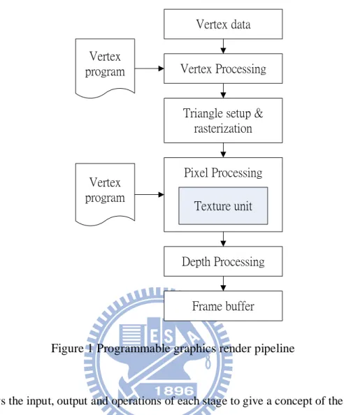
Figure 1 is the programmable graphics render pipeline, we discuss the render pipeline in several parts, which are vertex processing, rasterization, pixel processing and depth processing.

Vertex Processing

Triangle setup & rasterization Texture unit Pixel Processing Depth Processing Frame buffer Vertex data Vertex program Vertex program

Figure 1 Programmable graphics render pipeline

Table 1 shows the input, output and operations of each stage to give a concept of the graphics pipeline. Then we introduce the detail operations of each stage in the follow sub-sections.

Table 1 Input, output and operation of each stage

Stage Input Output Operation

Vertex Processing Vertices coordinates of primitives Vertices coordinates of primitives in eye’s viewing Transform coordinates ModelWorldeye Triangle Setup and Rasterization Vertices of primitives

Fragments Interpolates each information of triangle into numbers of fragments

Pixel Processing Fragments Fragments Colors each fragment according to its information

Depth Processing

Fragment with final color and depth value

Image composed of pixels

Stored color of pixel which will showed in screen into frame buffer

1.1.1 Vertex Processing

Vertex processing is supported by vertex shader in GPU [3]. Vertex shader performs mathematics operations on the vertex data for objects by the vertex shader programs. Vertex data are the 3D coordinate values (which are x, y and z) for the vertex and an object consists of three vertexes. Vertex shader does several transformations and normalizations, which are model-view

transformation, projection transformation, Clipping, perspective division and viewport mapping. After the transformations and normalizations, the 3D based objects will be transformed into normalized 2D based objects on screen which all the coordinate values are in the interval 0 and 1. Then vertex processing sends the normalized 2D coordinate values to rasterization which will be introduced at next section.

1.1.2 Triangle Setup and Rasterization

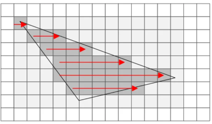
Rasterization receives the vertices data from vertex processing, then rasterize the fragments which are in the primitive. It uses horizontal scan line onto the primitive to produce fragments, which is showed below Figure 2.

Figure 2 Triangle rasterization

In the rasterization process, it also interpolated the x, y, and z coordinates and the color information like red, green, blue, alpha values.

1.1.3 Pixel Processing

Pixel processing is supported by pixel shader. Pixel shader receives fragments from rasterization stage and does computations for the fragments. Each fragment will be colored according to the pixel shader code, including texture mapping which we will introduce in section 1.2. After pixel

processing, the fragments with final color and z value will be sent to depth processing.

1.1.4 Depth Processing

Using frame buffer to store the pixel color which will be display on the screen. In this stage, z value of every pixel is compared with z value which has the same screen address (means has the same x, y values) of Z-Buffer. Z-Buffer is a buffer of screen-size using to store the nearest z value of every pixel [4]. If z value of the pixel is smaller than the value of the Z-Buffer, Z-Buffer is updated by the z value and frame buffer is updated by the new color. After depth processing, screen display the colors which are stored in frame buffer.

1.2 Texture Mapping and Texture Filtering

At this section, we will introduce an important technique in modern GPU which is called texture mapping. We will introduce two techniques used in texture mapping in the subsections which are called mip-map and texture compression.

1.2.1 Texture Mapping

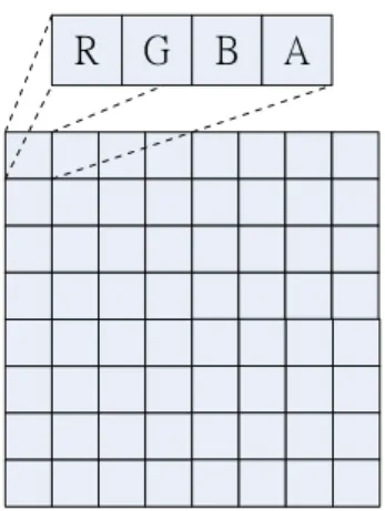
Before introducing texture mapping, we introduce texture first. Texture is a 2D bit-map image and its width and height are powers of two. The maximum size of texture supported in modern GPU is 4096×4096. Texel is the basic element of texture, it is consisting of four components which are Red, Green, Blue, and Alpha (or RGBA in short). RGB are the value of color and A id the value of transparency. Each component is one byte, which means that each texel is four bytes.

Figure 3 shows a texture, which width and height are all eight. It means the size of this texture is 4×8×8=256 bytes.

R G B A

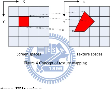
Texture mapping is a process, which make primitive realities and also reduce computations. It applied a texture to a primitive instead of using many primitives to make the object realities.

The number of required triangles is increased and thus the number computation is increased du to realize realistic a very complex image. But reduced the number of triangles means reduced the realistic quality of an object. Hence, to have more realistic object with less triangles, texture mapping has been used commonly in 3D computer graphics. Figure 4 shows the texture mapping operation between screen spaces and texture spaces.

X

Y

u

v

Screen spaces Texture spaces

Figure 4 Concept of texture mapping

1.2.2 Texture Filtering

In order to render textured scenes with good quality, some kind of texture filtering is needed. This is to avoid aliasing that can occur under minification, and avoid a block appearance under magnification. Figure 5 shows when the minification and magnification occurs, the footprint covered range of fragment.

X

Y

u

v

Screen spaces Texture spaces

Figure 5 Left: when minification occurs the fragment footprint covers many texels, Right: when magnification occurs, few or only one texel is covered by the footprint

Due to the absence of no one-to-one mapping between texels and pixels, an interpolation calculation is necessary for high quality mapping. Higher quality requires computation intensive interpolation to generate a final pixel value from many texel values.

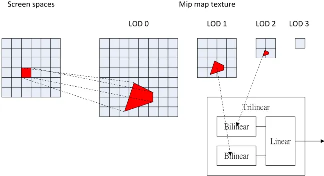
Commonly used texture filtering algorithms in current 3D games are bilinear filtering (Bi), trilinear filtering (Tri), and anisotropic filtering (Ani). There is a tradeoff between operation complexity and image quality among various texture filtering algorithms. Both trilinear and anisotropic support the mip-map technique. Mip-map is a technique to reduce the artifacts which arise from the use of a single bitmap image while the level of detail of an object decreases with an increase in the distance. Figure 6 shows the trilinear technique using mip-map texture.

LOD 0 LOD 1 LOD 2 LOD 3 Mip map texture

Screen spaces

Bilinear

Bilinear

Linear Trilinear

Figure 6 Concept of trilinear and mip-map texture

1.2.3 Texture Compression

In the section 1.2.2, we know texture is a very large bit-map image. Mip-map technique makes the storage almost double larger than normal texture. In order to render textured scenes with good quality, we needs more complex texture filtering technique and mip-map texture support, which means we need more storage to stored the texture and wide bus to transfer the textures data.

Texture compression solves the problem, it can use smaller storage to store the same texture and keep the quality after decompression good enough. With the texture compression

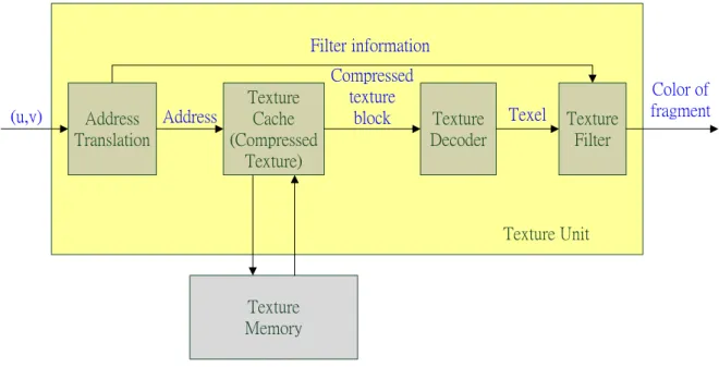
technique, we can store the compressed texture in the texture cache, and decompress the texture block we need to use for texture filter dynamically. Because the texture always stored in cache in compressed forms, which means we reduce the traffic between texture and texture unit. This technique let we can use the same memory and cache but we can stored more texture in memory and cache. Smaller storage and bandwidth required means smaller power consumption. Figure 7 shows the texture unit with texture compression technique.

Address Translation Texture Cache (Compressed Texture) Texture Filter Texture Decoder Texel Compressed texture block Filter information Texture Unit (u,v) Color of fragment Texture Memory Address

Figure 7 The texture unit with texture compression technique

Texture unit supports texture mapping operation in GPU. Texture unit is composed of an address translation, texture cache, texture decoder, and texture filter. Process of texture unit is that texture unit receives texture coordinate (u, v). Then address translation translates the texture coordinate (u, v) of texel into real address, then sends the address to texture cache to fetch texel. This action may active several times. After all the requested compressed texture block are sent to texture decoder, texture decoder will decompress the texture block and compute the colors that texture filter unit needs. Then the texture filter unit will compute the final color value according to the filter type and weight then sends the color value to pixel shader.

1.3 Motivation

The texture compression needs to decompress the texels from the compressed texture block dynamically. That means the decompress process should be easy in hardware and time. In slim devices such as cell phones, this request must be satisfied with limited silicon and

computing power.

Issues to be tackled under texture compression technique: 1. Compression ratio should be high.

2. Decompression should be easy in hardware and time. 3. Quality of result should be high.

Compression ratio and quality after decompress is a tradeoff, that means high compression ratio usually means the quality after decompress is bad. But we still want the decompression should be easy. It is a hard work to target the issue above, but we want challenge to target all the issues above.

S3TC is a renowned texture compression technique. In its RGB format, 64 bits are used to represent a block of 16 texels with 8-bit RGB, resulting in 24*16/64=6 compression ratio. However, some difficulties exist: its decompression requires division, whereas its

approximation hardware alternative loses precision. Other famous schemes include PVR-TC, iPACKMAN, etc.

Texture compression remains an important topic in computer graphics. Despite compression techniques, textures are consuming ever large proportions of the memory bandwidth. So to simplify the difficulties of S3TC is a good topic for us and in next section we will introduce the goals we want to target.

1.4 Objective

Design a texture compression technique, which can achieve the following goals:

1. Retain the same compression ratio since 64 bits are good figures, but record more color information if possible.

2. Simplify decompression hardware, and make the process quick. 3. Texture quality must be maintained if not raised

processing during texels retrieval. Characteristics of O2TC are list as bellow. 1. Compression ratio is six.

2. Exploiting binary virtues to improves the calculate equations.

3. Quality of result is -0.06 dB lower than theory of S3TC and the 0.25dB differences is visible by human eyes.

4. Produces 16 texels on one time decompress in best case.

1.5 Thesis Organization

The origination of follow sections in this thesis is: Chapter 2 introduces background of related works. Chapter 3 introduces our O2TC design, including Option1 and Option2 design and texture with alpha channel design. Experiment results are shown in chapter 4. Discussion and conclusion are made in chapter 5.

Chapter 2 Background

In this chapter, we will introduce the texture compression methods which our O2TC rest on. The texture compressions which we will introduce are BTC, CCC, S3TC and iPACKMAN. We will introduce how they compress the texture and decompress the texture.

2.1 Block Truncation Coding

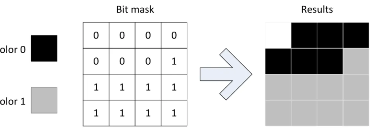
Delp and Mitchell [5] developed a simple scheme, called block truncation coding (BTC) for image compression. Their scheme compressed gray scale images by a block of 4x4 pixels. The method represents a block by two 8-bit gray scale value and index map. Everything is

contained in the codeword, no global data or color palette needs to be read. However, BTC having only two base colors of gray gives rise to banding artifacts. This allowed for

compression of texture at 2 bpp. Although, the applications of BTC were not the texture compression, many other proposed texture compression method are based on their ideas. Figure 8 shows the concept of BTC.

0 0 0 0 0 0 0 1 1 1 1 1 1 1 1 1 Base color 0 Base color 1

Bit mask Results

2.2 Color Cell Compression

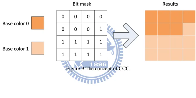
A simple extension of BTC to represent color images, called color cell compression (CCC) was proposed by Campbell et al [6]. They use 8-bit value as an index into a color palette. The method required storing a color palette for every texture and access memory twice for an indirect data. This allowed for compression of texture at 2 bpp. Knittel et al. suggested that it was implemented in the texturing hardware. Figure 9 shows the concept of CCC.

0 0 0 0 0 0 0 1 1 1 1 1 1 1 1 1 Base color 0 Base color 1

Bit mask Results

Figure 9 The concept of CCC

2.3 S3 Texture Compression

The further extension of CCC, called S3 Texture Compression (S3TC) was proposed by Iourcha et al [7]. The S3TC is probably the most popular standard today. It is used in DirectX and OpenGL. The S3TC represents a 4x4 block by four 16 bits (RGB565) base color and each pixel stores an index with 2 bits. Two base colors are stored in the compressed block and the others are linearly interpolated from those two during the decompression process. Figure 10 shows the concept of S3TC. This means that all colors lie on a line in RGB space.

Color 00 Color 01 Color 10 Color 11 00 00 10 01 00 10 11 01 10 11 01 01 01 01 00 00

Original block Look-up Table Bit mask

Derived

Results

Figure 10 The concept of S3TC

The interpolate equations show bellow.

C10 =(2×C00+1×C₃ 01) (1.a)

C11 =(1×C00+2×C₃ 01) (1.b)

The equation shows it must has divided by 3 operation, that means either implement the divider unit or using approximation equations instead of divided operation. The S3 graphics proposed the approximation equations show bellow.

C10 =5×C₈00+3×C₈01 =1×C₂00 +1×C₈00 +1×C₂01−1×C₈01 (2.a)

C11 =3×C₈00+5×C₈01 =1×C₂00 −1×C₈00 +1×C₂01+1×C₈01 (2.b)

The equations implement in hardware is simpler than divided by 3 operations, but it also lost many precision in interpolated the colors C10 and C11. S3TC allowed for compression of

texture at 4 bpp.

2.4 iPACKMAN

PACKMAN has been improved under the name iPACKMAN (also call Ericsson Texture Compression, ETC [8]) in two ways. First and most important, a differential mode is

introduced, allowing two neighboring 2x4 blocks to be coded together. The base color of the one block can be encoded using RGB555 instead of RGB444. Another block also encoded in RGB555 format, but coded using a differential value in dRdGdB333 format. The second improvement is that blocks can be flipped. One block consists of either two 2x4 block or two

4x2 block. These change improved 2.5dB in terms of Peak Signal to Noise Ratio (PSNR).

Figure 11 shows a possible iPACKMAN decompressor.

Figure 11 The decompressor design of iPACKMAN

2.5 Discussion

Base on the above listed texture compression methods; we can understand that loosely compression order to pursue more rapid decompression is also a relative sacrifice the quality of the images. We tried to find a faster method of decompression, but not sacrifice more quality. The quality after decompression of S3TC is good enough, but the operations are

complicated. Follow the S3TC method, maybe we can exploit another faster decompression method. With the faster decompression method, another important thing is how to found the optimal base colors. Next chapter we introduce our ideas and implementation.

Chapter 3 Design

In this chapter, we will introduce our design of texture compression and decompression system. We will introduce two kinds of design which are inter/extrapolation mode (Option1 in short) and advanced differential mode (Option2 in short). Then, we will introduce how to encode the texture and how to handle the texture with alpha channel using our design.

3.1 Basic Ideas

At this section, we introduce the differences between O2TC and other texture compression method. The main goal of our proposed design is to both simplify texture decompression operations and keep the same quality as S3TC.

To achieve the goal, we propose the Order-of-Two Texture Compression (O2TC) that takes the full advantage of binary system to reduce complexity in run-time decompression while acquiring the most quality. The most noticeable feature of our design is that we exploit as much of the beauty of binary system as we can, include the following:

1. Devise as many of our operations into such as divide-by-two, and implement it with skewed wiring—no shifter will ever needed

2. Order colors/alpha values in ascending or descending order, whichever gives better maintained quality, since binary add of positive or negative numbers are identically performed.

3. Choose larger valued colors to be our base colors, or even record different bit fields for color difference if a medium color and difference pair is used, to maintain more color information using the same bit count.

3-operand add, or even use all 2-operand adds in our decompression

5. Retrieval of block texels can easily be parallelized, since all texels can individually be computed from compressed information without much redundancy.

6. Assume an implicit 1 as the next data bit of compressed color components, to minimize color truncation error bound and raise quality if retrieved texture.

Circuit and timing analyses show that O2TC is superior to S3TC in hardware requirement, while experiment results show average PSNR (peak signal-to-noise ratios) of 35.84 and 35.83 for O2TC Option1 and Option2, and 35.39 for S3TC DXT1. With alpha values, the quality of 128-bit O2TC is far better: average PSNR of O2TC Option1 and Option2 and S3TC DXT5 are 40.42, 39.55, and 37.62 in our test cases, in addition to O2TC’s circuit and timing advantages.

3.2 Inter/Extrapolation Mode

We start look at S3TC first, and see how S3TC needs complex operation in decompression work. Figure 12 show the colors C0 and C3 are stored as base colors when off-line compression. And dynamically computation the addition indexed colors C1 and C2 using interpolation. C0, C1, C2, C3 are the base colors of the block, which are calculated by PCA or LGB algorithm. The interpolation formulas are listed bellow.

C0 = C0 (3.a) C1 =(2×C0+1×C3)₃ (3.b) C2 =(1×C0+2×C3)₃ (3.c) C3 = C3 (3.d)

We can see clearly a complex divided by 3 of operation in the formulas that will cause heavy effort in the decompression process.

C0 C1 C2 C3

Figure 12 Stored color of S3TC

We want to reduce the complexity of computation of S3TC. To replace the complex divided by 3 of operation with other easy way is the most important work we need to do. Then we found that the differential value computed from (C3.R-C0.R)/3 is equal to the value of (C2.R-C0.R)/2. It is for this reason that we selected C2 as the base color instead of C3 and stored in compression bits. Then we can use fast and low cost right shift operations instead of complex and expansive division operation in the decompression process.

The basic inter/extrapolation mode of O2TC has proposed. The color C0 and C2 are selected as base colors and stored in compression. Thus, the additional indexed colors C1 and C3 can be computed by only using simple add and shift operations. The equations are

changed to list as bellow.

C0 = C0 (4.a) C1 = C0 +(C2−C0)₂ (4.b) C2 = C2 (4.c) C3 = C2 +(C2−C0)₂ (4.d)

Figure 13 shows the stored colors of basic inter/extrapolation mode of O2TC.

We can see a right shift operation in the formulas, which is easy use skewed wiring to implement in the decompression process.

C3

C0 C1 C2

3.2.1 Bits Layout

The texture image is split into many blocks which have 4x4 texels, where each block is represented by 64 bits, which is the same bit rate as S3TC. We have two base colors C0 and C2 and two additional indexed colors C1 and C3, so we need to stored 2 bits index for indexed the colors. There are 16 texels in one block, so we need 32 bits for stored the indices of texels. Thus, 32 bits remains, and two base colors are needed to store for each block.

Since the eye is more sensitive to green than to red and blue, it make sense (from a perceptual point of view) to let green come closer to its desired value, and worse representation of blue and red. The common luminance formula is defined as

Y(c) = 0.299cr + 0.587cg + 0.114cb (5) It is for this reason that we stored a single base color in 5+6+5 = 16 bits RGB (or RGB565 for short). Then we total used 2(5+6+5) + 32 = 64 bits for represented one block. This allowed for compression of texture at 4 bpp. The Figure 14 shows the bits layout we used in basic inter/extrapolation mode of O2TC.

R0(5) G0(6) B0(5) R2(5) G2(6) B2(5)

Texel Indices (32)

Figure 14 Bits layout of compression in Inter/Extrapolation mode of O2TC

There are 24 bits for represented one base color in original bitmap format. But we just have 16 bits for represented one base color in RGB565 format. Thus, we stored the five most significant bits (MSB for short) of red, six MSB for green and five MSB for blue. Figure 15 shows the bits we stored for one base color.

7

6

5

4

3

2

1

0

7

6

5

4

3

2

1

0

7

6

5

4

3

2

1

0

Figure 15 Bits stored of red, green and blue of one base color

3.2.2 Errors computation

In this section, we introduce how to decode the base color that can obtain the minimum error between original color and color after decompression process. First, we considered the red component of one base color. In the above section, we save the 5 MSB of red, but in the decompress process we need to do something to increase the quality during decompress process instead of padding three zero bit. In the S3TC, they padding the 3 MSB of code word of red component that seems good idea, but any other method will improve the process? One red component has 8 bits that has 256 kinds of permutation. We have two base colors and two addition base colors, so if we want to calculate the error of all possible composes then we need to calculate 65536 times. We try to calculate the error of padding the tree MSB of code word and padding b100 for all kinds of composes, then we got the result shows that the average error of padding the tree MSB of code word is 1.94 and the average error range of padding b100 is 1.69. It clearly let we known padding b100 will got more advantage then the tree MSB of code word. Figure 16 shows the range of three bits represents, and b100 and b011 are the middle values of the range, so padding b100 is padding the average error.

0 0 0

0 0 1

0 1 0

0 1 1

1 0 0

1 0 1

1 1 0

1 1 1

4 3

Figure 16 The range that padding b100 presented

3.2.3 Texture decompression

In this section, we start to design the decoder circuit for inter/extrapolation mode of O2TC. Figure 17 illustrates a possible hardware design diagram for a decompressor of

inter/extrapolation mode of O2TC. Below we describe in more detail how a single texel is decompressed using such hardware.

CWR

(10)

CWG

(12)

CWB

(10)

Texel

Indices

(32)

Z

R

Which texel

(4bits)

...

2

I0 and I1

Decoder C S A + C L A Y 1 0 U X 6 0 0 6 6 5 5 0 0 8

G

C S A + C L A Y 1 0 U X 7 0 0 7 7 6 6 0 8

B

C S A + C L A Y 1 0 U X 6 0 0 6 6 5 5 0 0 8 R0 R2 G0 G2 B0 B2

Figure 17 This diagram shows a possible decompressor of basic Inter/Extrapolation mode of O2TC

Table 2 The true table of control signals and results of computation in basic inter/extrapolation mode of O2TC I1 I0 X U Y Value 0 0 0 0 0 R0 0 1 1 1 0 R0+(R2-R0)/2 1 0 0 0 1 R2 1 1 1 1 1 R2+(R2-R0)/2

1. First, the code words need to be obtained. Four input bits from are used to select which texel of the decompressed block to decompress using MUX (Multiplexer unit) Z. The resulting 2 texel index bits are I1 and I0.

2. We should either use the five bit value R0 directly, in which case MUX X chooses zero, MUX U chooses zero and MUX Y chooses R0, or we should use the sum R0+(R2-R0)/2, in which case MUX X chooses R2, MUX U chooses R0 and MUX Y chooses R0, or we should use R2 directly, in which case MUX X chooses zero, MUX U chooses zero and MUX Y chooses R2, or we should the sum R2+(R2-R0)/2, in which case MUX X chooses R2, MUX U chooses R0 and MUX Y chooses R2.

3. The final step computes the final decompressed color by adding the outputs of MUX Y, MUX X and MUX U. Before add operation, the output of MUX Y should padded with a one-bit to fit the six bit adder, the output of MUX X should padded with a zero-bit and the output of MUX U should padded with a zero-bit. No clamping is necessary since the encoded process can make sure these values never overflow.

According to the TRUE table list in Table 2 of control signal, we can summarizes the control signal of MUX X, MUX U and MUX Y are show as below

X = U = I0 (6.a) Y = I1 (6.b) The control signal is very simple to implement, or we can say that just the wire routing and

don’t need any logical gates.

3.2.4 Parallel Decompression

In this section, we introduce how to sending out all colors for the 16 texels of the compressed texture block in parallel. Figure 18 shows the design of O2TC Option1 decompressor. Only 5-bit red component is shown for simplicity. Given C0 and C2, the decompressor calculates C2 and C3 using a 2-Color Generator (whose detail are shown in the lower part of Figure 18). Note that all shifts are implemented with skewed wiring, and

padding bits are either 1 or 0 to minimize error bounds. It also pads 5-bit and 6-bit color components of C0 and C2 with 100b or 10b to generate 8-bit RGB C0 and C2 (not show in Figure 18). Texel indices are then used to select among the 4 representative colors to generate the 16 block texel colors in parallel, such a design has both major advantages in timing and power. These are due to that colors need to be calculated only once, the arithmetic is

extremely simple, and the 16 texel colors are retrieved simultaneously. With CSA and CLA, the 3-input adder should not become a serious speed bottleneck.

C0_RGB565 Texel_Indices(32) 2 - Co lo r G en er at o 2 C2_RGB565 2 x 4 Decoder _C0 C1 C2 C3 T 15 … … … … … … 2 2 x 4 Decoder T 14 2 2 x 4 Decoder T 13 2 2 x 4 Decoder T 0 + C0_R5 C2_R5 C S A C L A IN V C0_R5 C2_R5 C2_R5 C1_R8 C3_R8 6 8 00 5 1 Cin 1 6 8 10 5 0 6 1 5 Red Channel of 2-Color Generator

Figure 18 O2TC option1 parallel texture retrieval circuit, with its 2-color generator show in the lower part

3.2.5 Discussion of inter/extrapolation mode

In inter/extrapolation mode design, we can found that the hardware of the decoder is only three adders and ten multiplexers. The adder of the design is the three inputs adder and it could be implemented as the CSA and CLA combination, which means the design we propose, are simpler than the hardware of S3TC. There are seven adders and some multiplexer required in S3TC patent, and the patent of S3TC are reduced the computation of divided by 3

operation, which means the image quality after decompressor of S3TC patent is not equal to the original S3TC presented.

shorter than the S3TC patent and shorter than iPACKMAN proposed, because the time latency of iPACKMAN is two multiplexers, two adders and one clamper delays. It is quite clear that our system is very low hardware and time complexity.

The next section, we will introduce the other mode, is called advanced differential mode of O2TC. It can reduced the hardware and time complexity than inter/extrapolation mode of O2TC, but the quality is a little worst than inter/extrapolation mode.

3.3 Advanced Differential mode

To further fast and simplify decompression work, advanced differential mode of O2TC is proposed. With this method, only one base color C1 and the differential value dC which is pre-computed by encoder are stored in off-line compression. Figure 19 shows colors stored in advanced differential mode of O2TC, or called Option2 of O2TC in short. With this

pre-computed value dC, the additional indexed colors can be calculated faster by easier hardware design. The interpolated equations are list as bellow.

dC = (C3 − C0)/3 (7.a) C0 = C1 − dC (7.b) C1 = C1 (7.c) C2 = C1 + dC (7.d) C3 = C1 + 2 × dC (7.e)

C0

dC

C1 C2 C3

3.3.1 Bits Layout

The texture image is split into 4x4 blocks, where each block is represented by 64 bits, which is the same bit rate as basic inter/extrapolation mode. We have one base color C1 and

differential value dC, that needed to stored in compression bits. In this mode we also need 32 bits for stored the indices of texels. Thus, 32 bits remains, and one base colors and one differential value are needed to store for each block.

We stored the only one base color in RGB565 is the same with basic inter/extrapolation mode. But how we should stored the differential value. Let we consider the range of differential value. We can found that it must larger than -255/3 and smaller than +255/3, because the largest value case is that C3.R = 255 and C0.R = 0 and the smallest value case is that C3.R = 0 and C0.R = 255. From the equation dC.R = (C3.R-C0.R)/3, then the value of differential value dC.R is larger than -85 and smaller than +85.

If we want keep the precision, we need eight bits for stored the dC.R, but we just have 16 bits for stored the value. In view of the difference of the colors in the block is very small in the general textures or pictures. We can reduce the bits to 7 bits for represented dC.R, and can also keep the quality almost equal to stored full 8 bits for represented dC.R.

It is for this reason that we stored the 2 to 6 bit of dC.R in five bits, stored the 1 to 6 bit of dC.G in six bits, and stored the 2 to 6 bit of dC.B in five bits. Figure 20 shows the bits we choose for stored the only one base color and the differential value of advanced differential mode of O2TC. Figure 21 shows the bits layout of compression in Option2 of O2TC.

7

6

5

4

3

2

1

0

7

6

5

4

3

2

1

0

7

6

5

4

3

2

1

0

7

6

5

4

3

2

1

0

7

6

5

4

3

2

1

0

7

6

5

4

3

2

1

0

C1 dC

Figure 20 Bits stored of red, green and blue of Option2 of O2TC

R1(5) G1(6) B1(5)

dR(5)

dG(6) dB(5)

Texel Indices (32)

Figure 21 Bits layout of compression in Option2 of O2TC

Another method for stored differential value has proposed and called Option2_EXT of O2TC. We consider the dC must larger than -85 and smaller than +85 and 8 bits signed integer can represent -128 to +127. One method that we can just addition +42 if dC >=0 and subtract 42 if dC<0. Then, subtract 42 if dC >=0 and addition 42 if dC <0 in decompression dynamically. This method can let we keep all value range that dC could occurs but we just have 16 bits for stored dC. Thus, we stored dC.R[3..7], dC.G[2..7] and dC.B[3..7]. Figure 22 shows the bits stored of Option2_EXT of O2TC.

This two method we proposed can used for many application depend on what kinds of feature you want. Option2 of O2TC is adapted for the natural pictures or normal textures, and Option2_EXT of O2TC is adapted for the pictures and textures with high contrast or high dynamic range.

7

6

5

4

3

2

1

0

7

6

5

4

3

2

1

0

7

6

5

4

3

2

1

0

7

6

5

4

3

2

1

0

7

6

5

4

3

2

1

0

7

6

5

4

3

2

1

0

C1 dC

Figure 22 Bits stored of red, green and blue of Option2_EXT of O2TC

3.3.2 Encode and errors computation

In this section, we introduce how to decode the differential value that can obtain the minimum errors between original color and color after decompression process. In Option2 of O2TC, we store dC.R[2..6]. Then, we could calculate the average errors when dC.R >-63 and dC.R < 63. The average errors is 2.3125. Then we can also calculate the average errors range when dC.R < - 63 && dC.R > - 85 and dC.R > 63 && dC.R < 85. The average errors range is 15. Figure 23 shows the range that padding 10b presented and from Figure 3-13 we can know ∆dR is between -1 to 2. The maximum errors is 27 that will occur when ∆R1 = 4 and ∆dR = 25.

In Option2_EXT, we can also calculate the average errors range and maximum errors range by modify the color’s errors equations. From calculation, we got the average errors range is 2.95 and maximum errors range is 6. It let we know that Option2_EXT can cover all the possible value of dC but it also lost some precision. In Option2 of O2TC, it will bring very large errors if dC.R > 63 or dC.R < -63, but it could not happen in Option2_EXT of O2TC. It is just a tradeoff problem and choice the right method by your applications.

the average errors range smaller than Option2_EXT. First, we assume the probability is x of dR is between -63 to +63 and that’s average errors range is 2.3125. Then we got the equation as bellow.

2.3125x + 15(1 − x) < 2.95 (8) From the equation 8, we can know when x > 0.95 that the average errors range of Option2 will smaller than of Option2_EXT.

1 2

0

0

0

1

1

0

1

1

Figure 23 The range that padding b10 presented

3.3.3 Texture decompression

In this section, we start to design the decoder circuit for advanced differential mode of O2TC. Figure 24 illustrates a hardware diagram for a decompressor of advanced differential mode of O2TC. Below we describe in more detail how a single texel is decompressed using such hardware.

Table 3 The true table of control signals and results of computation in advanced differential mode of O2TC I0 I1 Value X0 X1 Y 0 0 R0 0 0 X 0 1 R0-dR 0 1 1 1 0 R0+dR 0 1 0 1 1 R0+2*dR 1 0 0 CWR (10) CWG (12) CWB (10) Texel Indices (32)

Z

Which texel

(4bits)

...

2

I0 and I1

Decoder X 1 6 5 0 0 6 6 5 C L A

R

0 0 8 Y Sign extension X 1 7 6 0 0 7 7 6 C L A

G

0 8 Y Sign extension X 1 6 5 0 0 6 6 5 C L A

B

0 0 8 Y Sign extension R1 dR G1 dG B1 dB

1. First, the base color and the differential value needs to be obtained. Four input bits are used to select which texel to decompress using MUX Z. The resulting 2 texel index bits are I0 and I1. We should either use the five bit value R0 directly, in which case MUX X chooses zero, or we should use the sum R0-dR, in which case MUX X chooses dR, or we should use the sum R0+dR , in which case MUX X chooses dR, or we should the sum R0+2dR, in which case MUX X chooses 2dR. In the case dR needs to do sign extension before multiplexer operation for fit the six bits MUX X. In the case 2dR we can be done inexpensively by padding with a zero-bit instead of left shift operation.

2. The final step computes the final decompressed color by adding the outputs of MUX X, and the base color. The controls signal Y that controls the adder for doing add or sub operation. No clamping is necessary since the encoder can make sure these values never overflow.

According to the TRUE table list in Table 3 of control signal, we can summarizes the control signal of MUX X and Control signal Y are show as below

X0 = I0 AND I1 (9.a) X1 = I0 XOR I1 (9.b) Y = NOT I0 (9.c) The control signal is very simple to implement, just few logical gates can finish the job.

3.3.4 Parallel Decompression

The Figure 25 shows the decompressor of Option2 of O2TC for parallel processing. Here the differences lie in that only one base color is readily available in the code word, and three other representative colors need to be calculated. No 3-input adder id need here. As discussed earlier. We might choose to use more bits for base color and fewer for the difference. Design changes to the corresponding decompressor are simple.

Red Channel of 3-Color Generator C1_RGB565 Texel_Indices(32) 3 - Co lo r G en er at o r 2 dC_RGB565 2 x 4 Decoder _C0 C1 C2 C3 2 x 4 Decoder 2 x 4 Decoder T 15 … … … … … … 2 x 4 Decoder -C1_R5 dC_R5 C0_R8 00 5 1 2 2 2 T 14 T 13 T 10 5 6 8 + C1_R5 dC_R5 C2_R8 00 5 1 5 6 8 + C1_R5 dC_R5 C3_R8 00 5 1 5 6 8 0

Figure 25 O2TC Option2 parallel texture retrieval circuit, with its 3-color generator show in the lower part

3.3.5 Discussion of advanced differential mode

In advanced differential mode design, we can find that the hardware of the decoder is only three adders and four multiplexers. The adder of the design can be implemented as the CLA , which means the hardware is much simpler than the basic inter/extrapolation mode.

The time complexity of advanced differential mode is only one adder and one multiplexer delay, and it can shorter than the basic inter/extrapolation mode, because in this mode we using two inputs adder instead of three inputs adder in basic inter/extrapolation mode.

design or mobile phone. The quality is just a little less than basic inter/extrapolation mode in 0.02 dB, but better than S3TC patent. This means that human should not notice the differences between using basic inter/extrapolation mode and advanced differential mode. But human will be notice the differences between using advanced differential mode and S3TC patent, because the quality is better than S3TC in 0.4 dB. To put this in perspective, a common rule of thumb used in the image compression community says that 0.25dB makes for a visible difference.

3.4 Texture encode

In this section, we introduced the process of off-line compression. The problem of compression is to find the best pairs of base colors.

Iterating over all possible base colors which have 232 different combinations would have to be tried for each block. It is not a good idea, so we need other algorithms to solve the problem. S3TC using PCA method to find the base colors of block instead of exhaustive search, and THUMB proposed LBG algorithm and Radius compression. The radius compression is much slower than LBG compression, but will also give a better result.

Radius compression is based on LBG algorithm, initially, two base colors are found using the LBG algorithm. Then for each quantized base color, all possible colors within a

(2k + 1) × (2k + 1) × (2k + 1) cube centered around the base color are tried. Usually using k=1 and is 729 times slower than LBG compression.

We try the PCA and Radius compression for each block and choose the smaller errors pair base colors. Following details the block compression of Option1 of O2TC:

1. Get a block and compression it into two 64-bit code words by recording two RGB565 base colors and setting the 16 texel indices using both increasing and decreasing color orders.

2. Simulate decompressions of the two code words, and calaulate their RMSE ( root mean square errors):

RMSE = �_{w × h � ∆R}1 xy2 + ∆Gxy2 + ∆Bxy2 xy

3. Save the code words with lower RMSE in compressed texture file. Figure 26 shows the first three steps of the algorithm.

4. Exit if no more block to compress; else go to step 1.

Option2 of O2TC follows the same procedure, with the only difference in the recorded color information: one base color and a color difference will record in the two code words using both increasing and decreasing color orders.

Encode block with (C0 , C2) if Option1 (C1 , dC) if Option2 then decode the colors of block

Start

Calculate the RMSE of block (E0)

End

Find two extreme colors (C0 , C3) using PCA Calculate another two colors (C1 , C2) using Interpolation

If (E0<E1)

Store (C0 , C2) if Option1 (C1 , dC) if Option2 as base colors Else

Store (C3 , C1) if Option1

(C2 , dC) if Option2 as base colors Encode block with (C3 , C1) if Option1 (C2 , dC) if Option2 then decode the colors of block

Calculate the RMSE of block (E1)

Figure 26 Base colors selection flowchart in texture block compression

3.5 Texture with Alpha channel

is also support texture with alpha channel. The same idea used in color

compression/decompression applies here. DXT5 stored A0 and A7 as two base colors. Figure 27 shows the stored colors. The decompression equations list as bellow. Note that DXT5 have divided by 7 operations and it is not hardware friendly.

dA = (A7 − A0)/7 (10.a) Ai = A0 + i × dA, i = 1. .6 (10.b)

A0 A1 A2 A3 A4 A5 A6 A7

Figure 27 Alpha channel compression/decompression of DXT5

In contrast to DXT5 codeword, we choose to use A0 A4 or A0 A8 (where A8 is an extrapolated alpha value) pair as base alpha values. We use A0 A4 in the following for simplicity. Figure 28 shows the stored colors. The interpolation equations list as bellow.

A0 = A0 (11.a) A1 = A0 +(A4−A0)₄ (11.b) A2 = A0 +(A4−A0)₂ (11.c) A3 = A0 −(A4−A0)₄ (11.d) A4 = A4 (11.e) A5 = A4 +(A4−A0)₄ (11.f) A6 = A4 +(A4−A0)₂ (11.g) A7 = A4 +(A4−A0)₂ +(A4−A0)₄ (11.h) A0 A1 A2 A3 A4 A5 A6 A7

Figure 28 Alpha channel compression/decompression of Option1 of O2TC

and adders of 2 or 3 inputs. Note that A7 may use a 4-input adder, which requires one CSA, adding come delay. This corresponds to Option1 for colors, and alpha values can again be ordered in increasing or decreasing order. The Option2 stored a base alpha A3 or A4 and a difference dA = (A7-A0)/7. Figure 29 shows the stored colors. The interpolation equations list as bellow.

dA = (A7 − A0)/7 (12.a) A0 = A4 − 3 × dA (12.b) A1 = A4 − 2 × dA (12.c) A2 = A4 − 2 × dA (12.d) A3 = A4 − 1 × dA (12.e) A4 = A4 (12.f) A5 = A4 + 1 × dA (12.g) A6 = A4 + 2 × dA (12.h) A7 = A4 + 3 × dA (12.i)

dC

C0 C1 C2 C3 C4 C5 C6 C7

Figure 29 Alpha channel compression/decompression of Option2 of O2TC

3.5.1 Bits layout

In Option1 of O2TC with alpha channel, we choose to store two base colors A0 and A4. In DXT5, the RGB format is the same as DXT1, and alpha channel format is 64 bits, where 16 bits are for two base alpha values and 3*16=48 bits for 16 texel alpha indices.

In our Option1 of O2TC, we first plain use 64-64 method. Two base alpha values A0 and A4 are stored instead of A0 and A7. Figure 30 shows the compression format with alpha.

C0_RGB565(16)

C4_RGB565(16)

Texel_RGB_Indices (32)

C0_A(8)

C4_A(8)

Texel_Alpha_Indices (48)

Figure 30 Option1 of O2TC with alpha – a plain 64-64 format

Then, we consider tuning the 128 bits format for better texture quality. Several possible Option1 type RGBA formats are designed and evaluated. Examples are: Letting RGB use more bits (e.q., RGB each uses 8 bits—the RGB888 option) to retain higher color precision, or inter/extrapolating more representative colors (e.q., use eight representative colors—the 8-color option) to offer more color choices. Figure 31 shows our best-effort RGBA tradeoff format. Experiments show its PSNR is 2.8dB better than DXT5 using ideal division.

C0_RGB565(16) C4_RGB565(16)

Texel_Alpha_Indices (32) C0_A(8) C4_A(8)

Texel_RGB_Indices (48)

Figure 31 O2TC Option1, the 8-color format with alpha

Option2 type 8-color format, an alternative with the best result in our effort, is represents in Figure 32.

C0_RGB565(16)

C7_RGB565(16)

Texel_RGB_Indices (32)

C0_A(8)

C7_A(8)

Texel_Alpha_Indices (48)

Figure 32 O2TC Option2, the 8-color format with alpha

3.6 Overall Design

In this section, we introduce the overall design block of O2TC. In the header of the compressed image file, we store the information of what kind of O2TC that the image used and support alpha or not. Figure 33 show the overall design of O2TC. Below we describe in

more detail how a block is decompressed.

1. First, obtain the 64 bits data from texture cache. The first 32 bits (0-31) are transfer to both of option1 of O2TC and option2 of O2TC decompression modules and last 32 bits (32-63) are transfer to alpha channel of O2TC.

2. MUX X select which color that will output, dependent on system defined 3. Output red, green, blue and alpha value to render the texel.

We have three basic block option1 of O2TC, option2 of O2TC, and alpha channel of O2TC. The system will be defined what method used, option1 or option2. Then, the blocks of texture will decompression one after another.

64 bits data ( with alpha)

X

Option1 of O2TC Option2 of O2TC Alpha channel of O2TC

Latches of color or alpha

0-31 32-63

Chapter 4 Experiment Results

In this chapter, we will introduce the quality after decompression, decompressor circuit and timing complexities of different compression methods.

4.1 Simulation Environment

In comparing texture quality, for 64-bit color-only code words, O2TC Option1, Option2, S3TC DXT1, PACKMAN, iPACKMAN, and PVR-TC are tested on seven images: five Kodak images, Lena, and Lorikeet. This seven images are also tested on others method before and we list the quality results of they proposed. For 128-bit RGBA code words, both O2TC options together with their alternatives and DXT5 are tested using 5 texture maps with alpha channel. For circuit and timing complexities, we examine only circuits for colors using 64-bit code words.

4.2 Quality Measure

The quality measure that we use is Peak Signal to Noise Ratio (PSNR), which is defined as PSNR = 10log10�3×255

2

RMSE2� (12)

Where the scale factor 3 in the numerator is due to the fact that 3×2552 is the peak energy in a pixel, and RMSE is the Root Mean Square Error, defined as

RMSE = �_w×h1 ∑ �∆Rx,y 2xy + ∆Gxy2 + ∆Bxy2 � (13)

Where w and h are the width and the height of the image, and △Rxy, △Gxy, △Bxy are the

green, blue component respectively.

4.3 Software Simulation Results

In this section, we compare color qualities of various methods. Various padding methods and various code words format, S3TC DXT1, PACKMAN, iPACKMAN, and PVR-TC are tested on same images.

4.3.1 Various padding methods

In comparing color qualities of various padding methods, we compare two methods, padding several MSB like S3TC, or padding average errors. Table 4 shows the quality results of Option1 of O2TC using various padding methods.

Table 4 Quality comparison of padding variations

Kodak img1 Kodak img2 Kodak img3 Kodak img4 Kodak img5 Lena Lorikee t Averag e Padding several MSB 34.69 36.73 38.5 37.96 32.82 35.89 34.32 35.84 Padding average errors 34.72 36.8 38.54 37.96 32.83 35.89 34.32 35.87

Padding average errors has better quality result, in comparison with padding several MSB like S3TC. In section 3.2.2 we also compare two methods in mathematical analysis. Both of two methods are simply to implements and hardware cost are just wiring issue.

4.3.2 Various code words format

We compare several variations of O2TC Option2, and choose a better variation for

comparison with other methods. Table 5 shows the quality results of O2TC Option2 variations

Table 5 Quality comparison of O2TC Option2 variations

Kodak img1 Kodak img2 Kodak img3 Kodak img4 Kodak img5

Lena Lorikeet Average

C1(6,7,6) + dC(4,5,4) 26.04 32.08 32.33 32.54 23.82 31.46 30.71 29.85 C1(6,6,6) + dC(5,5,4) 26.98 33.14 33.46 33.49 24.62 32.13 31.19 30.72 C1(5,6,5) + dC(5,6,5) V1 34.41 36.42 37.83 37.36 32.52 35.55 34 35.44 C1(5,6,5) + dC(5,6,5) V2 34.71 36.88 38.39 37.86 32.74 35.92 34.28 35.83 C1(6,7,6) + dC(4,5,4) V2 29.43 33.81 34.48 34.89 26.57 33.81 32.8 32.26

In C1(5,6,5)+dC(5,6,6) V2, dR[7..3], dG[7..2], dB[7..3] are stored in codeword, Some least significant color difference bits are dropped, losing some precision. This method is an obvious winner and will be used in later comparisons.

4.3.3 Various 64 bits methods

We then compare the color qualities of various methods. We mentioned that S3TC DXT1 calculates color difference using ÷ a very expansive operation, or approximation to simplify circuit design. We call them S3TC_Theo and S3TC_Impl, respectively. Table 4-2 shows the PSNR results of different methods. As a result, the PSNRs of O2TC Option1 and Option2 are both better than S3TC_Impl, even with simpler hardware. iPACKMAN has the best PSNR in Table 6, but according ETC2 reports the PSNR of iPACKMAN is the same with S3TC. Table 6 is the special case of iPACKMAN. Figure 34 shows the PSNR results of various methods.

Figure 34 PSNR results of various methods

Table 6 Quality comparison of O2TC Option2 variations

Kodak img1 Kodak img2 Kodak img3 Kodak img4 Kodak img5

Lena Lorikeet Average

PACKMAN 33.81 34 35.37 35.5 32.35 33.56 31.73 33.76 S3TC_Theo 34.78 36.82 38.53 37.79 32.8 35.97 34.37 35.86

S3TC_Impl 34.06 36.45 37.91 37.42 32.24 35.62 34.06 35.39 PVR-TC 33.8 37.1 37.9 37.7 32.4 35.9 34.8 35.66 iPACKMAN 36.29 38.08 38.62 38.59 34.12 35.17 33.25 36.30 O2TC Option1 34.68 36.75 38.52 37.93 32.81 35.87 34.34 35.84 O2TC Option2 34.71 36.88 38.39 37.86 32.74 35.92 34.28 35.82

4.3.4 Various 128 bits methods with alpha channel

Next we compare retrieved texture qualities of different methods with alpha included using 128-bit codewords. We use S3TC DXT5_Theo, giving it some advantage. Results are shown in Table 7. All O2TC versions perform better than DXT5_theo, and the best O2TC is 2.8dB better (shows in Figure 35).

Figure 35 PSNR of various methods with alpha

Table 7 Quality comparison of DXT5_Theo and various O2TC

Bush_1 Bush_2 Chainlink Tree1 Tree2 Average

O2TC_Plain64-64_Option1 36.08 38.58 42.49 35.9 35.82 37.774 O2TC_RGB888_Option1 36.32 38.83 42.57 36.17 36.06 37.99 O2TC_8-color_Option1 38.56 41.2 46.34 37.53 38.49 40.424 O2TC 8-color_Option2 37.64 39.89 44.94 37.12 38.17 39.552

4.4 Timing and Circuit Complexity Analyses

Table 8 lists the hardware component counts, complexity, critical path latency, and timing complexity, together with retrieved texel quality of various methods. Here we assume O2TC circuits to decompress a texel at a time. From this table, one can see that O2TC has both hardware and timing advantages, and its quality is only inferior to the more expansive iPACKMAN.

As the described before, O2TC is very well suited to parallel texel retrieval. Although its parallel version data are not presented in above table, we argue that the time-space behavior of its parallel versions will be very attractive.

Table 8 Timing and circuit complexity of various one-texel-at-a-time retrieval methods

Ideal S3TC S3TC Patent iPACKMAN Option1 of O2TC Option2 of O2TC C om pon e nt s Divider 1 0 0 0 0 Adder 1 7 6 3 3 Multiplexer 2 3 8 10 4 Codebook 0 0 1 0 0 Clamp 0 0 3 0 0

Hardware Complexity High Medium Medium Low Very Low

1 adder 1 divider

2 MUX 2 MUXes 1 clamp

1 MUX 1 MUX

Time Complexity High Medium Low Low Very Low

Chapter 5 Discussion and Conclusion

5.1 Evaluations and Discussion

O2TC intends to explore virtues of binary representations and arithmetic. In its

compression and decompression, we examine every detail, and devise our methods to achieve better quality and cheaper process. Experimental results have shown that out efforts are well rewarded. We compare the average quality, hardware component, time latency of Option1 and Option2 of O2TC and S3TC patent list in Table 9

Table 9 Quality, hardware, timing comparison of Option1 and Option2 of O2TC and S3TC

Average quality

Hardware components

Time latency parallelism

S3TC_Impl 35.39 7 adders + 3 Multiplexers 3 adders + 2 multiplexers No Option1 of O2TC 35.84 3 adders + 10 Multiplexers 1 adder + 1 multiplexer Yes Option2 of O2TC 35.83 3 adders + 4 Multiplexers 1 adder + 1 multiplexer Yes

In addition to above, we also studied the best uses of the limited compressed codeword space. We suggested to eliminate storage of redundant bits such as duplicated sign bits in a difference, and allocate more bits—borrowed from alpha channel—to the three colors. This also has been proven useful. In response to this bits relocation and format variations, field shifting and wire routing strategies are also discussed. In the next step, we will implement this

idea into silicon, and measure the real parameters.

5.2 Conclusion and Future Work

Texture and image compression/decompression is an important enabler for many applications. Design challenges lie in how to obtain high compression ratio while keep run-time decompression easy and quality after it high. We describe our research work in this thesis. Our efforts indicate that there are opportunities for improvements, based or the great contributions of previous works. Complete solutions of the O2TC compression and

decompression, together with many variations, are presented.

We are trying to give O2TC more mode, e.g.,H-, T-, and Planar-modes as in ETC2 and studying its relationship with memory hierarchies, and applying it to mip-mapping and applying it to high dynamic range textures.