NIG-GARCH選擇權訂價模型

(1)

國立交通大學

財務金融研究所

碩士論文

NIG-GARCH 選擇權訂價模型

On The NIG-GARCH Option Pricing Model

研究生：黃兆輝

指導教授：李昭勝教授

(2)

NIG-GARCH 選擇權訂價模型

On The NIG-GARCH Option Pricing Model

研究生：黃兆輝 Student：Chao-Hui Huang

指導教授：李昭勝教授 Advisor：Dr. Jack C. Lee

國立交通大學

財務金融研究所

碩士論文

A Thesis

Submitted to Graduate Institute of Finance National Chiao Tung University in partial fulfillment of the requirements

for the Degree of Master

in

Finance

June 2005

Hsinchu, Taiwan, Republic of China

(3)

NIG-GARCH 選擇權訂價模型

研究生:黃兆輝

指導教授:李昭勝

國立交通大學財務金融研究所

摘要

這篇論文發展了一個誤差項服從由 Barndorff-Nielsen (1997) 所提出之 Normal Inverse Gaussian 分配來做 GARCH 選擇權訂價模型。這個模型叫做 NIG-GARCH 且將包含 Duan (1995)之 GARCH 選擇權訂價模型為其極限特例。此外吾人也提出另一個可考慮到“槓桿效應＂現象之 NIG-NGARCH 模型，其可以解釋財務時間序列上常發生之資產報酬波動率不對稱的現象。在史坦普爾 500 指數的實證研究上顯示我們的模型檢驗比 Duan (1995) 和 Heston and Nandi (2000)之 GARCH 模型還要好。而另一個在史坦普爾 500 指數選擇權訂價上的研究也顯示我們的模型在比較價內的買權時優於其他的 GARCH 模型。這改善是由於“厚尾分配＂假設所致，且因此可以解釋財務時間序列上“超越峰態＂的現象。

(4)

On The NIG-GARCH Option Pricing Model

Student:

Chao-Hui

Huang

Advisor:

Jack

C. Lee

Graduate Institute of Finance

National Chiao Tung University

Abstract

This thesis develops a GARCH option pricing model with its innovation following a Normal Inverse Gaussian (NIG) distribution as proposed by Barndorff-Nielsen (1997). The model is called NIG-GARCH and will include the GARCH option pricing model of Duan (1995) as a limiting case. In addition, we also consider the “leverage effects” in the model, called NIG-NGARCH, which can explain the asymmetric effect of asset return volatility, observed often in financial time series. Empirical studies on S&P500 index shows that model checking of our models perform better than the GARCH models of Duan (1995) and Heston and Nandi (2000). Studies on pricing S&P500 index options also shows that our model in the out-of-sample performance is superior to other models for at-the-money calls. The improvement is due to the distribution with fat tails and thus can explain excess kurtosis often observed in financial time series.

(5)

Acknowledgements

研究所兩年的日子很快就過去，在交大財金所的專業訓練下得以充實基本的功力，無論在財務、統計、數學、電腦都有所獲。首先要感謝我的指導教授李昭勝博士，李老師在統計界頗負盛名，能夠得到老師的細心指導是我最大的福氣。另外，我要感謝統計所博士班牛維方學長的照顧，無論是在電腦程式或者是財金專業的知識上都能夠給予我許多的教導與指正，以學長本身的豐富經驗讓我得以順利完成本篇論文。而口試時感謝政大廖四郎教授、交大鍾惠民副教授、及台中技術學院林淑惠副教授給予一些寶貴的意見，讓本篇論文更為完善。畢業之際，許多回憶湧上心頭，感謝碩士班同學們在求學的路上一起成長，有了你們讓我獲益良多。當中經歷過許多的歡笑與淚水，特別是感謝我家的貓兩年內的陪伴與照顧，讓我在研究所的生涯畫上完美的句點。也感謝養育了我二十四年的父母親，讓我從小到大無憂無慮的過完求學生活，沒有你們就沒有今天的我，而心中的感謝更是無法言語。僅將本篇論文獻給我最愛的父母親以及所有的師長和朋友

們。

黃兆輝謹誌於國立交通大學財務金融研究所中華民國九十四年六月二十五日

(6)

1. Introduction

Since the seminal paper on the autoregressive conditional heteroskedasticitic (ARCH) model introduced by Engle (1982), various works on the financial time series have been dominated by the extensions of the ARCH process. Bollerslev (1986) extended the work of Engle to the generalized autoregressive conditional heteroskedasticitic (GARCH) process to include past conditional variances in the current conditional variance equation. The GARCH process can capture the empirical regularities observed in the time series data such as “volatility clustering “. Duan (1995) developed a GARCH option pricing model that relaxes the assumption of constant volatility in Black and Scholes (1973) formula.

However, the GARCH process fails to explain the characteristics of “leverage effects” often observed in financial time series. The concept of leverage effects, first discovered by Black (1976), refers to the tendency for changes in stock returns to be negatively correlated with changes in returns volatility. In other words, the impact of the “good news” is different from the impact of the “bad news” volatility, i.e., volatility tends to rise in response to “bad news” and to fall in response to “good news”. Duan, Gauthier and Simonato (1999) used nonlinear asymmetric GARCH (NGARCH) of Engle and Ng (1993) to obtain an analytical approximation for option pricing model which is similar to the Black and Scholes formula with adjustments used for skewness and kurtosis. Heston and Nandi (2000) developed a closed-form solution for European option values in GARCH model which simultaneously captures path dependence in volatility (volatility clustering) and the negative correlation of volatility with asset returns (leverage effects).

However, financial time series exhibit excess kurtosis in empirical studies. Therefore, the assumption of Gaussian innovation seems inappropriate for financial time series. In addition to the Gaussian distribution, several alternative innovation distributions had been proposed in the early GARCH literature, including the t-distribution proposed by Bollerslev (1987), the Generalized Error Distribution (GED) proposed by Nelson (1991), and the Normal Inverse Gaussian (NIG) distribution proposed by Andersson

(8)

(2001) and Bollerslev (2002). These distributions have fatter tails than the Gaussian distribution and can be used to explain excess kurtosis. But, there is no literature proposed properly about GARCH option valuation with innovations following the NIG distribution. In this thesis, we propose a model combining the GARCH option valuation and innovations for the asset returns following the NIG distribution. The model is called NIG-GARCH and will include the GARCH option pricing model of Duan (1995) as a limiting case. In addition, the “leverage effects” is also considered in our model called NIG-NGARCH.

There are two parts in our empirical studies. One is the empirical studies on daily returns of S&P 500 index that we can use standardized innovations (or called standardized residuals) of stock returns to check the model assumption. Another is the empirical studies on S&P 500 (SPX) index call options that we use three loss functions to compare the out-of-sample performance. We choose the GARCH option pricing models of Duan (1995) and Heston and Nandi (2000) as benchmark models. The former result is that our models can well fit the daily returns on S&P 500 index because only our models follow the distribution assumption. The latter result is that our model is superior to other models for at-the-money calls and does not perform too badly for in-the-money or out-of-the-money calls. Besides, we also find that non analytical solution GARCH-type models can fit the observed implied volatility of call option data much better than the closed-form model.

The remainder of this thesis is organized as follows. In section 2, we introduce the distribution, process and GARCH model of the normal inverse Gaussian. We then construct the NIG-GARCH option pricing model and describe the parameter estimation in section 3. Section 4 shows the empirical study. Finally, section 5 concludes.

(9)

2. The Normal Inverse Gaussian distribution and GARCH Model

2.1 The Normal Inverse Gaussian distribution

The normal inverse Gaussian (NIG) distribution proposed by Barndorff-Nielsen (1997) is useful for statistical modeling, particularly in finance. It is characterized by four parameters

(

α β μ δ, , ,

)

, whereα stands for steepness, β for symmetry, μ for location, and δ for scale. Consider a pair of random variables X and Z, the marginal distribution of X is normal inverse Gaussian where

(

,

)

,

X Z

=

z

∼

N

μ β

+

z z

(2.1a)

Z ∼IG( , ),δ γ (2.1b)

_γ₌ _α2₋_β2_,0_≤ _{β α μ}_< _, _∈ _and _δ_>0. _(2.1c)

LetIG( , )δ γ denote the inverse Gaussian distribution with probability density function (pdf) 2 2 3 2

( ; , )

exp

,

2

IG

f

z

δ

γ

δ

δ γ

γ

π

−

⎧

⎪

⎛

⎞

⎫

⎪

=

_⎨

−

_⎜

−

_⎟

_⎬

⎝

⎠

⎪

⎩

⎭

(2.2)

then the pdf of NIG( , , , )α β μ δ is

( )

0 1 1 ( ; , , , ) exp NIG Z X Z f x f x z f z dz x x x q K q

α β μ δ

α

μ

_αδ

μ

_{δ γ β}

μ

π

δ

∞ − = ⎧ ⎫ − ⎧ − ⎫ ⎡ − ⎤ ⎛ ⎞ ⎛ ⎞ ⎛ ⎞ = _⎜ _⎟ _⎨ _⎜ _⎟_⎬× _⎨ _⎢ + _⎜ _⎟_⎥_⎬ ⎝ ⎠ ⎩ ⎝ ⎠⎭ ⎩ ⎣ ⎝ ⎠⎦⎭

∫

(2.3)

and its moment generating function (M.G.F.) is

(

_{; , , ,}

)

_exp

{

(

2 ₍ ₎2

)

}

X

(10)

where _{q x}

( )

₌ ₁₊_x2 _, _γ ₌ _α2₋_β2 _and 1( )

K x is the modified Bessel function of second kind (also called third order by some researchers) and index 1. A special case of NIG distribution is normal distribution_N_{( ,}_{μ σ}2₎_{which corresponds to}_β ₌_0,_α_{→ ∞ and}

2_.

δ _σ

α= Set β =0, δα =σ2 and αδ η= , then (2.1) become

X Z = ∼z N

(

μ

, ,z

)

(2.5a) _Z_∼_IG₍_{σ η}2_{, ),} _(2.5b)

where >0.η

Let_IG₍_{σ η}2_{, )}_{denote the inverse Gaussian distribution with pdf}

2 ₃ 2 2 ₂ 2 1 ( ; , ) exp , 2 2 IG z f z z z

ησ

η

σ η

η

π

σ

− ⎧⎪ ⎛ ⎞⎫⎪ = _⎨ − _⎜ + _⎟_⎬ ⎪ ⎝ ⎠⎪ ⎩ ⎭ (2.6)

then the pdf of _NIG₍_σ2_{,0, , )}_{μ η} _is

( )

2 0 1 1 2 1 1 1 2 2 ( ; ,0, , ) exp NIG Z X Z f x f x z f z dz x x q K q

σ

μ η

η

_η

μ

_η

μ

πσ

_ση

∞ − = ⎧ ⎫ ⎛ ₋ ⎞ _⎪ ⎛ ₋ ⎞_⎪ ⎜ ⎟ ⎜ ⎟ = _⎜ _⎟ _⎨ _⎜ _⎟_⎬ ⎪ ⎪ ⎝ ⎠ ⎩ ⎝ ⎠⎭

∫

(2.7)

and its moment generating function is

(

_; 2_{,0, ,}

)

_exp

{

(

2 2 2

)

}

_. X M u σ μ η = uμ η+ − η ησ− u (2.8) Asη→ ∞ , then

( )

_exp 2 2 2 X M u = ⎛_⎜uμ+σ u ⎞_⎟ ⎝ ⎠ (2.9)

(11)

which is M.G.F. of _N

(

_{μ σ}_, 2

)

_. _{By the uniqueness of M.G.F., we can see that normal}

distribution is a limiting case of NIG distribution. In order to model time-varying conditional variance, let μ and β be 0 and assume that

(

0,

)

, t t t t X Z = ∼z N z (2.10) and

(

2

)

1 , , t t t Z Ω ∼₋ IG σ η (2.11) then

(

)

(

)

(

2

)

1 ₀ 1 1 ( ) , ,0,0, NIG t t t t t t t t t f x Ω₋ =

∫

∞ f x z Ω₋ f z Ω₋ dz ∼NIG σ η (2.12) where _IG

(

_{σ η}2_,

)

_and_NIG

(

_σ2_,0,0,_η

)

_{are given by (2.6) and (2.7)}

and

Ω is the information set of all information up to and including time t. _t

2.2 The Normal Inverse Gaussian GARCH Model

Consider a one-period rate of return for the underlying asset and let St be the asset price at time t and ht be the conditional variance of the log return over time interval [t-1, t]. Assume price process under the physical measure P can be modeled as following:

1 1 ln 2 t t t t t S r g g S₋ = − +λ + ε (2.13) where ₂

(

2

)

t t

g = η− η η− h and ε_t is a sequence of independent random variables with mean zero and variance h ; r is the constant one-period risk-free interest rate and _t λ could be interpreted as “excess return with respect to a risk-free investment per unit of risk” or called the unit risk premium.

(12)

Traditionally,ε_t is assumed normally distributed with mean zero and variance_σ2_.

Duan (1995) assumes that ε_t conditional on the information set Ω is normally _t distributed with mean zero and varianceh , which follows a _t GARCH p q process of ( , )

Bollerslev (1986) under measure P. We assumes that ε_t conditional on the

information set Ω is normal inverse Gaussian with mean zero and variance _t₋₁ h , which _t follows a nonlinear asymmetric GARCH (NGARCH) model proposed by Engle and Ng (1993) under P-measure as below:

1

(

,0,0,

)

P

t t

NIG h

t

ε

Ω ∼

₋

η

(2.14)

h_t = +w α ε

(

_t₋₁−θ h_t₋₁

)

2+βh_t₋₁

where θ is a non-negative parameter to capture the negative correlation between the innovations of asset return and its conditional volatility. The parametric restrictions ofw>0,α ≥0,β≥ ensures that conditional volatility is non-negative. And, to ensure 0 that the unconditional variance of asset return is bounded (or covariance stationarity) the parameter restriction_α

(

₁₊_θ2

)

_{+ < is required. From (2.16) the unconditional variance}_β ₁

can be derived:

ω

(

1 −

α

(1

+

θ

2

)

−

β

)

.

(2.15)

Combining (2.13) and (2.14), we label this model as NIG-NGARCH (1, 1). Ifθ = , we 0 call the model as NIG-GARCH (1,1). By taking the limit of η approach infinity, the GARCH (1,1) option pricing model of Duan (1995) is a limiting case of NIG-GARCH(1,1) and the NGARCH (1,1) option pricing model is also a limiting case of NIG-NGARCH (1,1). The Black-Scholes model is also a special case of NIG-GARCH (1,1) as η approach infinity, α = and0 β = . 0

(13)

3. The GARCH-Type Option Pricing Model

There are two kinds of discrete time GARCH models to value the European option. One is the nonanalytical solution for option values which use Monte-Carlo simulation to compute the option prices. Another is the closed-form solution which uses the inversion formula of Heston and Nandi (2000) in terms of the characteristic function. The former is usually used to compute the option price in empirical work but it takes more time than the latter. The GARCH –type option pricing models are presented in next two sections. 3.1 The NIG-GARCH Option Pricing Model

In order to develop the GARCH option pricing model, Duan(1995) introduced the locally risk-neutral valuation relationship (LRNVR) as a counterpart of the conventional risk-neutral argument extended in Rubinstein(1976) and Brennan (1979). From another economically meaningful assumption thatS_t Ω essentially does not allow _t₋₁ the arbitrage profits, which we can just profit with risk free rate or can be written

as

(

₁

)

₁ r

t t t

E S Ω− =S e− . Under this risk-neutralized probability measure Q, the price

process in (2.13) and (2.14) becomes

* 1

1 ln

2

t t t t

S

r

g

S

₋

= −

+

ε

(3.1) and * 1

(

,0,0,

)

Q t t

NIG h

t

ε

Ω ∼

₋

η

(3.2)

(

*

)

2 1 1 1 1 t t t t t h = +w α ε₋ −θ h₋ −λ g₋ +βh₋ where * t

ε conditional on Ω is a normal inverse Gaussian with mean zero and _t₋₁ varianceh . (3.1) is risk-neutral and can easily be showed in appendix C. The risk-neutral _t NIG-NGARCH (1,1) option pricing model contains six parameters η , ω , α , β , θ , λ . From (3.1) we can easily derive the following terminal asset price:

(14)

T T * T t j j j=t+1 j=t+1

1 =S exp (T t)r

g +

.

2 S

⎡

_⎢

−

ε

⎤

_⎥

⎣

∑ ∑

⎦

(3.3)

The principle of no arbitrage (or called the law of one price) indicates that a European call option with strike price K and expiring at maturity T must have the following value at time t:

C

_tNIG-NG

= e

−r(T t)−

E

_Q

⎡

_⎣

max (S

_T

−

K , 0)

Ω ⎤

_t

_⎦

.

(3.4) where

E

Q

[]

denotes the expectation under the risk-neutral distribution. By letting η

approach infinity, from (3.1) to (3.4) also converge to GARCH option pricing model of Duan under measure Q. Since the option price can’t be derived analytically, Monte Carlo simulations are used to compute the approximate option prices.

3.2 The Heston-Nandi GARCH Option Pricing Model

Another famous discrete-time pricing model is the Heston-Nandi GARCH option valuation model (2000). They developed a closed-form solution for European option values in GARCH model which simultaneously captures path dependence in volatility (volatility clustering) and the negative correlation of volatility with asset returns (leverage effects). Considering the Heston-Nandi GARCH (1,1) process that asset price process under measure P is defined as

1

ln

t

,

t t t t

S

r

h

h z

S

₋

= +

λ

+

(3.5) 2 1 1 1 ( ) , t t t t h = +ω α z₋ −γ h₋ +βh₋

wherew>0,α≥0,β≥ ; 0 z is standard normal random variable; r is the constant _t one-period continuously compounding interest rate. The parameter γ controls the skewness or the asymmetry of the distribution of the log returns. Under the risk-neutralized probability measure Q, the asset price process in (3.5) become

(15)

*t 1

1 ln

2

t t t t

S

r

h

h z

S

₋

= −

+

(3.6) * * 2 t-1 1 1 ( ) , t t t h = +ω α z −γ h₋ +βh₋ where *t t t

1 z =z +

+

h ,

2 λ

⎛

⎞

⎜

⎟

⎝

⎠

*_{= + + .}1 2 γ γ λ

If the characteristic function of the log spot price is f( φi ), then a European call option with strike price K and expiring at maturity T is worth the following value at time t:

[

]

( ) HN t Q ( ) _* 0 * ( ) 0 C max( ,0) 1 ( 1) = Re 2 1 1 ( ) Re , 2 r T t T r T t _i t i r T t E S K K f i S d i K f i Ke d i

e

φ φ

φ

_φ

π

φ

_φ

π

φ

− − − − ₋ ∞ − ∞ − − = − ⎡ + ⎤ + _⎢ _⎥ ⎣ ⎦ ⎛ ⎡ ⎤ ⎞ − _⎜ + _⎢ _⎥ _⎟ ⎣ ⎦ ⎝ ⎠

∫

(3.7)

where

f i

( )

φ

can be obtained from the conditional moment generating function ( )f φ by substituting iφ for φ,

(

)

T

( )

[

]

exp

( ; , )

( ; , ) ( 1),

t t

f

E S

S

A t T

B t T

h t

φ φ

φ

=

+

(3.8) where,

( ; , )

( 1; , )

1 ln(1 2

( 1; , ))

2 A t T

A t

T

r B t

T

B t

T

φ

φ φ

φ ω

α

φ

=

+

−

+

(3.9a)

(16)

2 2 1 ( ; , ) ( ) ( 1; , ) 2 1 (₂ ) , 1 2 ( ; , ) B t T B t T B t T φ φ λ γ γ β φ φ γ α φ = + − + + − + − (3.9b)

with the terminal conditions:

A T T

( ; , ) 0.

φ

=

(3.10a)

( ; , ) 0.

B T T

φ

=

(3.10b)

3.3 Parameter Estimation

In GARCH models, the most commonly used method in estimating the vector of

unknown parameters,

θ

, is the maximum likelihood estimates (MLE).

Assuming t

t

z = h

ε _{are independently and identically distributed standardized}

innovations with common density function f which has mean zero and variance one. The log-likelihood function can be expressed as

(

t

)

( )

t 1

1 ( )

log f(z )

log h

.

2

T t

l

θ

=

⎡

⎤

=

_⎢

−

_⎥

⎣

⎦

∑

(3.11)

If the density function f isNIG(1,0,0, )η (2.7), then log-likelihood function is

( )

1 1 2 t t 1 t 1 1 2 2 1

z

₁

( )

T

log

exp

₂

log h

t

l

θ

η

q

K

η

q

π

_η

− =

⎡

⎛

_⎛

_⎞

_⎧

_⎪

_⎛

_⎞

_⎫

_⎪

⎞

⎤

⎢

⎜

_⎜

_⎟

_⎜

_⎟

⎟

⎥

=

_⎢

_⎜

_⎟

_⎨

_⎜

_⎟

_⎬

−

_⎥

⎜

_⎝

_⎠

_⎪

_⎝

_⎠

_⎪

⎟

⎩

⎭

⎢

⎝

⎠

⎥

⎣

⎦

∑

(3.12)

( )

2 2 t t 1 t 1 z z 1 1 1

= T ₂log ( )-log( )+ ₂log (1+ )+ log (1+ ₂log h

t K η π η η η η = ⎡ ⎛ ⎛ ⎞⎞ ⎤ − − ⎢ ⎜ ⎜ ⎟⎟ ⎥ ⎢ ⎝ ⎝ ⎠⎠ ⎥ ⎣ ⎦

∑

(17)

where

θ

=

(

ω α β λ θ η

, , , , ,

)

for NIG-NGARCH (1,1). If the density function f is N(0,1), then log-likelihood function is

( )

2 t z 2 t 1

1

1 ( )

log

e

log h

2

T t

l

θ

π

− =

⎡

⎛

⎞

⎤

=

⎢

⎜

_⎜

⎟

_⎟

−

⎥

⎢

_⎝

_⎠

⎥

⎣

⎦

∑

(3.13)

( )

2

( )

t t 1 1 1 1 = log 2 z log h 2 2 2 T t π = ⎡₋ ₋ ₋ ⎤ ⎢ ⎥ ⎣ ⎦

∑

where

θ

=

(

ω α β λ θ

, , , ,

)

for NGARCH (1,1),

(

, , , ,

)

θ

=

ω α β λ γ

for HN-GARCH(1,1).

The parameters θ can be estimated by using numerical methods such as non-linear minimization as well.

(18)

4. Empirical study

4.1 Empirical study on stock index

We can check the adequacy of a fitted GARCH-type model by examining the series of standardized innovations

{ }

z

_t . First, using the Ljung-Box (LB)-Q statistic to check for serial correlation (autocorrelation) on the series of

{ }

z

_t and conditional heteroscedasticity (or called (G)ARCH effects) on the series of

{ }

z

2_t . The null hypothesis of the former is “no autocorrelation” and the latter is “no ARCH effects”. Second, using QQ-plot to check the distribution assumption. In addition, we can also use Jarque-Bera (JB) test to check

the normal assumption and Kolmogorov-Smirnov (KS) test to check the NIG assumption

on the series of

{ }

z

_t .

We use daily returns on S&P 500 index from July 1, 1988 to June 28, 1991 to

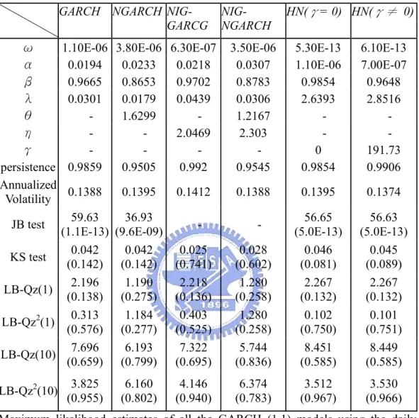
estimate the models’ parameters under measure P. Table 1 shows the maximum

likelihood estimates and some characteristics of the GARCH-type models. The annualized volatility (252days) of NGARCH (1,1) and NIG-NGARCH (1,1) is

(

2

)

252ω 1−α θ(1+ )−β and the Heston-Nandi GARCH(1,1) is ₂₅₂₍_{ω α}₊ _{) 1}

(

₋_αγ2₋_β

)

_.

All the GARCH models imply a 14% annualized volatility and Ljung-Box-Q statistic for testing autocorrelation and GARCH effect shows those models are adequate for the data at the 5% significance level.

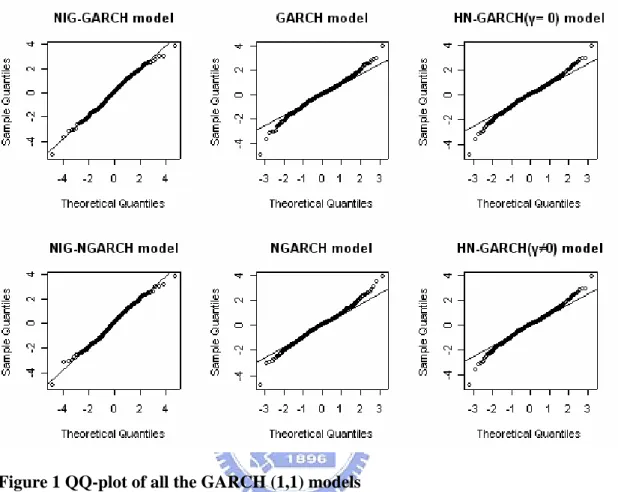
Figure 1 shows the QQ-plots of the six GARCH-type models on standardized innovations. We can find that the NIG-GARCH and NIG-NGARCH option pricing model can almost capture the empirical data. However, the GARCH models of Duan (1995) and Heston and Nandi (2000) can not capture the empirical data on the fatter tails which often observed in financial time series. Further evidence can be seen from the testing results in Table 1. The value of the Kolmogorov-Smirnov test statistic on the

(19)

NIG-GARCH and NIG-NGARCH are 0.025 and 0.028 with p-values 0.741 and 0.602 which do not reject the null hypothesis of NIG at the 5% significance level. The p-value of the Jarque-Bera test on GARCH model with normal assumption almost equal to zero that also rejects the null hypothesis of normality at the 5% significance level. Therefore, our model can well fit the daily returns on S&P 500 index.

4.2 Empirical study on Options

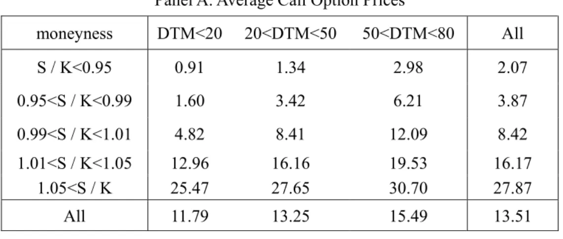
The previous section has already showed the empirical results on index data. We proceed to investigate the performance of these models on option pricing. Special attention is paid to the out-of-sample performance. For this empirical study, S&P 500 (SPX) index call options which are European-type and traded on the Chicago Board Options Exchange (CBOE) are considered. Because of the active market, S&P 500 index options have been included as illustrations in many researches, including Bakshi, Cao and Chen (1997), Dumas, Fleming and Whaley (1998), Heston and Nandi (2000) and so on. The data set here is identical to that of Bakshi, Cao and Chen (1997). We use call option contracts on 235 trading days from January 8, 1991 to December 31, 1991 and apply the same filters of Bakshi, Cao and Chen (1997). Table 2 gives the basic description on the options data including the average call option prices and the number of call option contracts across days to maturity (DTM) and moneyness. We restrict the maturities of option contract between 7 and 80 days and define the moneyness as S K where S is the S&P 500 index level and K is the strike price. Our call option data set contains 4324 option contracts and the average option price is $13.51. In next section we will discuss the interesting question on how to examine the models’ performance in out-of-sample analysis.

We analyze the out-of-sample performance by the following steps. First, the parameters of all the models are estimated from the previous three years’ S&P 500 index and forecast the next one month call option prices. Second, we roll the parameters every month and repeat step 1 twelve times then we can get the one year forecasted model option prices. We note that the parameters in one month (about 20 trading days) do not

(20)

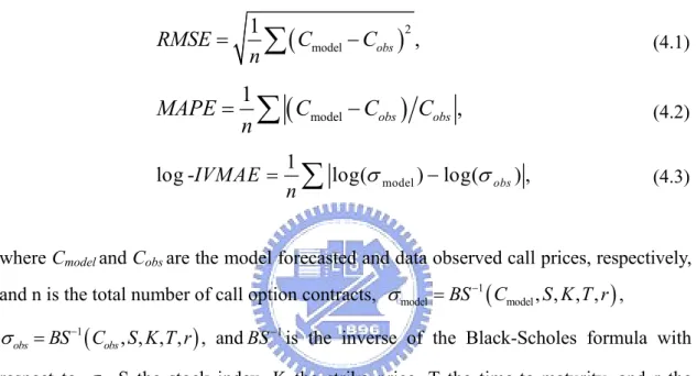
change significantly if the stock market structure does not vary largely. Finally, the forecasted option prices are plugged into the Black-Scholes formula to get the model-implied volatility. Then three loss functions in terms of the root mean square error (RMSE), the mean absolute percentage error (MAPE), and the mean absolute error of log-implied volatility (log-IVMAE) are calculated to evaluate the performance of different option pricing models. The loss functions mentioned above are defined as:

(

model

)

2

1 ,

obs

RMSE

C

n

=

∑

−

(4.1)

(

model

)

1 ,

obs obs

MAPE

C

n

=

∑

−

(4.2) model 1

log -IVMAE log( ) log( _obs) ,

n

σ

=

∑

− (4.3)

where Cmodel and Cobs are the model forecasted and data observed call prices, respectively,

and n is the total number of call option contracts, 1

(

)

model BS Cmodel, , , ,S K T r

σ ₌ − _,

(

)

1 _{, , , ,}

obs BS Cobs S K T r

σ ₌ − _{, and}_BS−1_{is the inverse of the Black-Scholes formula with}

respect to σ, S the stock index, K the strike price, T the time-to-maturity, and r the riskfree interest rate. The loss functions in (4.1) and (4.2) are the most commonly used in out-of-sample performance. However, there are some drawbacks in using the call price to compare the model performance. Using the RMSE loss function indeed puts much more weight on expensive options, such as in-the-money or long time-to-maturity call option contracts. On the other hand, using MAPE loss function puts much more weight on cheap options, such as out-of-money or short time-to-maturity call option contracts. Since the market convention is to quote in terms of volatility, some literature proposes alternative loss function to compare the model with the implied Black-Scholes volatility, such as PAN (2002), Christoffersen and Jacobs (2004).

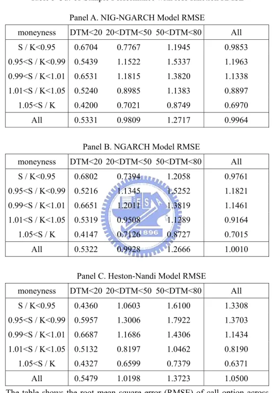
Table 3 shows the out-of-sample RMSE loss function across days to maturity and moneyness for NIG-NGARCH, NGARCH and HN-GARCH models during the

(21)

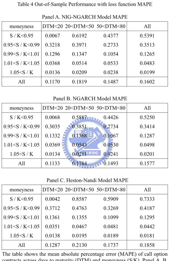
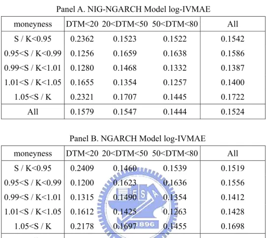
out-of-sample period from January 8, 1991 to December 31, 1991. The overall RMSE are 0.9964, 1.0010, and 1.0500 for the NIG-NGARCH, NGARCH and HN-GARCH, respectively. Through the overall RMSE we can know which model is best, but it does not reveal too much information. So, we report the RMSE by moneyness category which has some interesting results. First, the NIG-NGARCH model appears to have the smallest valuation error for at-the-money call options, NGARCH model has the smallest valuation error for (deep) out-of-the-money call options and the HN-GARCH model has the smallest valuation error for (deep) in-the-money call options. Second, the performance of HN-GARCH is worst for (deep) out-of-the-money call options and the NGARCH is worst for (deep) in-the-money call options. Generally specking, the NIG-NGARCH model’s performance is superior to other GARCH models for at-the-money calls and does not perform too badly for in-the-money or out-of-the-money calls. It is also true for the mean absolute percentage error (MAPE) and the mean absolute error of log-implied volatility (log- IVMAE) reported in Table 4 and Table 5, respectively.

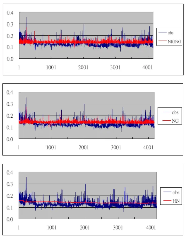
Figure 2 displays the data observed and model forecasted implied volatility where the horizontal axis is the number of call option contracts and the vertical axis is the annualized volatility (252 days). It shows that the model forecasted implied volatility of the NIG-NGARCH and the NGARCH can almost capture the data observed implied volatility. However, the forecasted implied volatility of the HN-GARCH model does not vary much over the number of call option contracts. As mentioned before, the GARCH model can capture the volatility clustering of return for the underlying asset. We also see that the forecasted implied volatility of nonanalytical solution GARCH models (NIG-NGARCH and NGARCH models) can fit the observed implied volatility of call option data. The HN-GARCH can capture path dependence in volatility of return, but it can not fit the observed implied volatility of call option data that indicates that there may be some question in this closed-form model.

(22)

5. Conclusion

This thesis proposes a model combining the GARCH option valuation and innovations for the asset returns following the NIG distribution. The model is called NIG-GARCH and will include the GARCH option pricing model of Duan (1995) as a limiting case. In addition, we also consider the “leverage effects” in the model, called NIG-NGARCH, which can explain the asymmetric effect of stock volatility. There are two results in our empirical studies. First, empirical results on index shows that our models can adequately fit the daily returns on S&P 500 index because the distribution assumption of normal inverse Gaussian has fatter tails than the Gaussian and can be used to explain excess kurtosis. Second, empirical results on call option shows that in out-of-sample performance our model is superior to the GARCH models of Duan (1995) and Heston and Nandi (2000) for at-the-money calls and does not perform too badly for in-the-money or out-of-the-money calls. Besides, we also find that although nonanalytical solution GARCH models take a lot of time in computing, they can fit the observed implied volatility of call option data much better than the closed-form models.

(23)

References

Andersen, J. (2001), “On the Normal Inverse Gaussian Stochastic Volatility Model,” Journal of Business and Economic Statistics, 19, 44-54.

Bakshi, G., C. Cao and Z. Chen (1997), “Empirical Performance of Alternative Option Pricing Models,” Journal of Finance, 52, 2003-2049.

Barndorff-Nielsen, O. E. (1997), “Normal Inverse Gaussian Distributions and Stochastic Volatility Modeling,” Scandinavian Journal of Statistics, 24, 1-13.

Barndorff-Nielsen, O. E. (1998), “Processes of Normal Inverse Gaussian Type,” Finance and Stochastics, 2, 41–68.

Barndorff-Nielsen, O. E. and N. Shephard (2001), “Non-Gaussian

Ornstein-Uhlenbeck-based Models and Some of their Uses in Financial Economics,” Journal of the Royal Statistical Society, Series B, 63, 167–241.

Barndorff-Nielsen, O. E. and Shephard, N. (2003), “Integrated OU Processes and non-Gaussian OU-based Stochastic Volatility,” Scandinavian Journal of Statistics, 30, 277-295.

Black, F. and Scholes, M. (1973), “The Pricing of Options and Corporate Liabilities,” Journal of Political Economy, 81, 637-654.

Bollerslev, T. (1986), “Generalized Autoregressive Conditional Heteroskedasticity, ” Journal of Econometrics, 31, 307-327.

Bollerslev T. (1987), “A Conditionally Heteroskedastic Time Series Model for

Speculative Prices and Rates of Return,” Review of Economics and Statistics, 69, 542–547.

Bollerslev, T. and Forsberg, L. (2002), “Bridging the Gap Between the Distribution of Realized (ECU) Volatility and ARCH Modelling (of the Euro): The GARCH-NIG Model,” Journal of Applied Econometrics, 17, 535-548.

Cox, J.C., Ross, S.A., and Rubinstein, M. (1979), “Option Pricing: a Simplied Approach,” Journal of Financial Economics, 7(3), 229-263.

Christoffersen, P., S. Heston and K. Jacobs (2003), “Option Valuation with Conditional Skewness,” Manuscript, McGill University.

Christoffersen, P. and K. Jacobs (2004a), “The Importance of the Loss Function in Option Valuation,” Journal of Financial Economics, 72, 291-318.

Christoffersen, P. and K. Jacobs (2004b), “Which GARCH model for Option Valuation?” Management Science, 50, 1204-1221.

(24)

Duan, J. C. (1995), “The GARCH Option Pricing Model,” Mathematical Finance, 5, 13-32.

Duan, J. C., G. Gauthier and J. Simonato (1999), “An Analytical Approximation for the GARCH Option Pricing Model,” Journal of Computational Financl, 2, 75-116. Dumas, B., J. Fleming, and R. Whaley (1998), “Implied Volatility Functions: Empirical

Tests,” Journal of Finance, 53, 2059-2106.

Engle, R. (1982), “Autoregressive Conditional Heteroskedasticity with Estimates of the Variance of UK Inflation,” Econometrica, 50, 987-1008.

Engle, R. and V. Ng (1993), “Measuring and Testing the Impact of News on Volatility,” Journal of Finance, 48, 1749-1778.

Heston, S. L. (1993), “A Closed Form Solution for Options with Stochastic Volatility, with Applications to Bond and Currency Options,” Review of Financial Studies, 6, 327-343.

Heston, S. L. and Nandi, S., (2000), “A Closed-Form GARCH Option Valuation Model,” Review of Financial Studies, 13, 585-625

Hull, J. and A. White (1987), “The Pricing of Options on Assets with Stochastic Volatility,” Journal of Finance, 42, 281-300.

Nelson, D.B. (1991), “Conditional Heteroskedasticity in Asset Returns: A New Approach,” Econometrica, 59, 347-370.

Pan, J. (2002), “The Jump-Risk Premia Implicit in Options: Evidence from an Integrated Time-Series Study,” Journal of Financial Economics, 63, 3-50.

Scott, L.O. (1987), “Option Pricing when the Variance Changes Randomly: Theory, Estimation and an Application,” Journal of Financial and Quantitative Analysis, 22, 419-438.

(25)

Appendix A. Tables

Table 1 Maximum likelihood estimates and Model characteristics

GARCH NGARCH NIG- GARCG

NIG- NGARCH

HN(γ= 0) HN(γ≠ 0)

ω 1.10E-06 3.80E-06 6.30E-07 3.50E-06 5.30E-13 6.10E-13

α 0.0194 0.0233 0.0218 0.0307 1.10E-06 7.00E-07 β 0.9665 0.8653 0.9702 0.8783 0.9854 0.9648 λ 0.0301 0.0179 0.0439 0.0306 2.6393 2.8516 θ - 1.6299 - 1.2167 - - η - - 2.0469 2.303 - - γ - - - - 0 191.73 persistence 0.9859 0.9505 0.992 0.9545 0.9854 0.9906 Annualized Volatility 0.1388 0.1395 0.1412 0.1388 0.1395 0.1374

JB test _(1.1E-13)59.63 _(9.6E-09)36.93 - - _(5.0E-13)56.65 _(5.0E-13)56.63 KS test _(0.142)0.042 _(0.142)0.042 _(0.741)0.025 _(0.602)0.028 _(0.081)0.046 _(0.089)0.045 LB-Qz(1) _(0.138)2.196 _(0.275)1.190 _(0.136)2.218 _(0.258)1.280 _(0.132)2.267 _(0.132)2.267 LB-Qz2(1) _(0.576)0.313 _(0.277)1.184 _(0.525)0.403 _(0.258)1.280 _(0.750)0.102 _(0.751)0.101 LB-Qz(10) _(0.659)7.696 _(0.799)6.193 _(0.695)7.322 _(0.836)5.744 _(0.585)8.451 _(0.585)8.449 LB-Qz2(10) _(0.955)3.825 _(0.802)6.160 _(0.940)4.146 _(0.783)6.374 _(0.967)3.512 _(0.966)3.530 Maximum likelihood estimates of all the GARCH (1,1) models using the daily returns on S&P 500 index from July 1,1988 to June 28,1991. The sample size of observations is equal to 756. JB test = Jarque-Bera test, KS test = Kolmogorov-Smirnov (KS) test, LB-Qz (p) = Ljung-Box Q test on autocorrelation for p lagged standardized innovations, LB-Qz2 (q) = Ljung-Box Q test on GARCH effects for q lagged squared standardized innovations. The parenthesis gives the p-value of all the tests.

(26)

Table 2 Basic description of Call Options data Panel A. Average Call Option Prices

moneyness DTM<20 20<DTM<50 50<DTM<80 All S / K<0.95 0.91 1.34 2.98 2.07 0.95<S / K<0.99 1.60 3.42 6.21 3.87 0.99<S / K<1.01 4.82 8.41 12.09 8.42 1.01<S / K<1.05 12.96 16.16 19.53 16.17 1.05<S / K 25.47 27.65 30.70 27.87 All 11.79 13.25 15.49 13.51

Panel B. Number of Call Options

moneyness DTM<20 20<DTM<50 50<DTM<80 All <0.95 2 84 70 156 [0.95,0.99) 210 712 339 1261 [0.99,1.01) 164 354 163 681 [1.01,1.05) 299 658 286 1243 >1.05 216 542 225 983 All 891 2350 1083 4324

The table shows the basic description of call option contracts written on the S&P 500 index for a total 235 trading days from January 8, 1991 to December 31, 1991. Panel A describes the average call option prices and Panel B describes the number of call options across days to maturity (DTM) and moneyness (S/K) where S/K is defined as the S&P500 index value over the option strike price.

(27)

Table 3 Out-of-Sample Performance with loss function RMSE Panel A. NIG-NGARCH Model RMSE

Panel B. NGARCH Model RMSE

Panel C. Heston-Nandi Model RMSE

The table shows the root mean square error (RMSE) of call option across days to maturity (DTM) and moneyness (S/K). Panel A, B, C stand for the models of NIG-NGARCH, NGARCH and HN-GARCH, respectively.

(28)

Table 4 Out-of-Sample Performance with loss function MAPE Panel A. NIG-NGARCH Model MAPE

Panel B. NGARCH Model MAPE

Panel C. Heston-Nandi Model MAPE

The table shows the mean absolute percentage error (MAPE) of call option contracts across days to maturity (DTM) and moneyness (S/K). Panel A, B, C stand for the models of NIG-NGARCH, NGARCH and HN-GARCH, respectively.

(29)

Table 5 Out-of-Sample Performance with loss function log-IVMAE Panel A. NIG-NGARCH Model log-IVMAE

Panel B. NGARCH Model log-IVMAE

Panel C. Heston-Nandi Model log-IVMAE

The table shows the mean absolute error of log-implied volatility (log-IVMAE) of call option contracts across days to maturity (DTM) and moneyness (S/K). Panel A, B, C stand for the models of NIG-NGARCH, NGARCH and HN-GARCH, respectively.

(30)

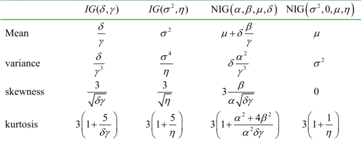
Table 6 Four characteristics for IG and NIG distributions IG( , )δ γ _IG₍_{σ η}2_{, )} _NIG

(

_{α β μ δ}_{, , ,}

)

_NIG

(

_σ2_{,0, ,}_{μ η}

)

Mean δ γ 2 σ μ δ β γ + μ variance δ₃ γ 4 σ η 2 3 α δ γ 2 σ skewness 3 δγ 3 η 3 β α δγ 0 kurtosis 3 1 5 δγ ⎛ ₊ ⎞ ⎜ ⎟ ⎝ ⎠ 5 3 1 η ⎛ ₊ ⎞ ⎜ ⎟ ⎝ ⎠ 2 2 2 4 3 1 α β α δγ ⎛ ₊ + ⎞ ⎜ ⎟ ⎝ ⎠ 1 3 1 η ⎛ ₊ ⎞ ⎜ ⎟ ⎝ ⎠

The IG and NIG denote inverse Gaussian and normal inverse Gaussian distribution,

respectively. The densities function of IG( , ),δ γ _IG₍_{σ η}2_{, ),} _NIG

(

_{α β μ δ}_{, , ,}

)

_and

(

2

)

(31)

Appendix B. Figures

Figure 1 QQ-plot of all the GARCH (1,1) models

The figure shows QQ-plot of the standardized innovations for daily returns on S&P 500 index from July 1, 1988 to June 28, 1991.

(32)

Figure 2 Implied volatility of data observed and model forecasted

The figure shows the implied volatility of data observed and model forecasted where obs is data observed implied volatility, NIGNG, NG and HN are model implied volatilities of NIG-NGARCH, NGARCH and HN-GARCH, respectively.

(33)

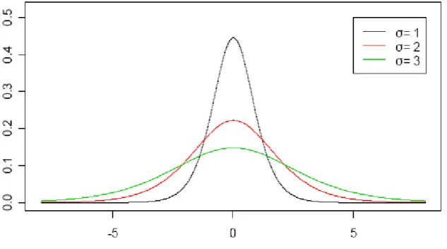
Figure 3a NIG densities with different σ

The figure shows NIG densities with β= 0,μ= 0,η= 3 andσ= 1, 2, 3 (from inner to outer).

Figure 3b NIG densities with different β

The figure shows NIG densities withσ= 1,μ= 0,η= 3 andβ= -1.6, -1, 0, 1, 1.6 (from left to right).

(34)

Figure 3c NIG densities with different μ

The figure shows NIG densities withσ= 1,β= 0,η= 3 andμ= -1, 0, 1 (from left to right).

Figure 3d NIG densities with different η

The figure shows NIG densities withσ= 1,β= 0,μ= 3 andη= 0.1, 0.5, 1, 2, 5 (from inner to outer).

(35)

Appendix C. Show that (3.1) is risk-neutral under measure Q Assuming ₁ 1 t t t S S − − Ω can be written as * 1

ln

t t t t

S

₋

=

μ ε

+

under measure Q whereμtis

the conditional mean and *

t

ε is NIG ( ,0,0, )h_t η process. As mentioned before, the M.G.F. of *

t

ε is

( )

_exp

(

2 2

)

t

M u = η− η η− h u , then we can derive that:

(

)

(

)

(

)

(

)

* * 1 1 1 1 1 2

exp

.

t t t t t t t t t t t t

S

E

E e

S

E e

h

μ ε μ ε

μ

η

η η

+ − − − − −

⎛

⎞

Ω

=

Ω

⎜

⎟

⎝

⎠

=

Ω

⎡

⎤

=

_⎢

+

−

_⎥

⎣

⎦

In order to make ₁ 1 t t t S S −

− Ω risk-neutral, using the relationship ₁ 1

r t t t S E e S₋ − ⎛ ⎞ Ω = ⎜ ⎟ ⎝ ⎠ we can

easily see that

(

2

)

t r ht

μ = − η− η η− . Therefore, we make sure that (3.1) is risk-neutral under measure Q.

NIG-GARCH選擇權訂價模型

國立交通大學

財務金融研究所

碩士論文