基於聽覺語言學與模糊類神經網路之英文母音辨識技術
61
0
0
全文
(2) 基於聽覺語言學與模糊類神經網路之 英文母音辨識技術. 學生:洪英士. 指導教授:周志成 博士 林進燈 博士. 國立交通大學電機與控制工程研究所 摘. 要. 在本論文中,我們提出一新的語者不相關的英文母音辨識技術。首先,我 們提出一組名為「聽學增強型-離散餘弦序列係數(AE-DCSC)」的新特徵。此特 徵的想法是將許多聽學語言學上有關英文母音的研究成果實現在頻譜的強化 上,讓其更具有代表性與差異化。其中,頻譜正規化(Spectrum-Level-Normalization) 用以平衡不同共振峰的高度差異。根據語言學的研究,共振峰的位置比其高度來 的重要。諧音的強化(Enhancement of Spectral Peaks)則能有效的壓抑介於諧音間 頻譜微小的變化,使其更具強健性。為了能在有限的特徵維度裡有效地保留母音 頻譜隨時間的變化情形,我們採用了離散餘弦序列係數這項技術。此技術具有可 改變的頻率與時間的彎曲比例,這讓我們能根據訊號的特性,找出最具有代表性 的特徵。而在本系統中,我們採用一前向式自我建構類神經模糊推理網路 (SONFIN)做為核心辨識器。利用其可自我建構並調整的架構與參數學習功能, 與優異的模糊類神經推論過程,來達到較佳之辨識效果。最後,我們提出一基於 語言學特徵的確認程序。針對較為混淆的辨識結果,擷取其在聽學語言學上的特 徵,並與我們事先建立的知識庫理的模型比對。以找出最可信的辨識結果。實驗 證明,在 TIMIT 的資料庫下,此系統的辨識率可達 74.75%,優於其他在文獻上 所見的結果。這說明了我們在此所提出的辨識系統所具有的潛力與優越性。. i.
(3) Speaker-Independent English Vowel Recognition Technique Based on Acoustic-Phonetics and Fuzzy Neural Networks Student: Ying-Shih Hung. Advisor:. Dr. Chi-Cheng Jou Dr. Chin-Teng Lin. Institute of Electrical and Control Engineering National Chiao-Tung University. ABSTRACT. In this thesis, we proposed a novel speaker-independent English vowel recognition technique based on acoustic-phonetics and fuzzy neural networks. At first, we proposed a new feature set called as “AE-DCSC”. It was derived from the researches of acoustic-phonetics and implemented here to enhance the spectrum so that the features became more representative and discriminative. The technique spectrum-level-normalization was used to balance the amplitude difference between formants. Moreover, the enhancement of spectral peaks was used to suppress the variation of valley between harmonics. These processes let the spectrum more robust and noise-free. In order to preserve the temporal cues of vowels, the technique DCSC was used. The flexible time/frequency warping scales were adjusted according to properties of signals. An on-line self-constructing neural fuzzy inference network (SONFIN) was adopted as the main classifier in this system. SONFIN found its optimal structure and parameters automatically and achieved the better classification result via superior inference process. Finally an acoustic-checking procedure was proposed. We applied it to the ambiguous case in which the acoustic characteristics was evaluated and compared with the model in our knowledge-base database. The proposed approach resulted in an accuracy rate of 74.75% in TIMIT database, which higher than other published result for the same task. The potential and effectiveness of the proposed system was verified.. ii.
(4) 致. 謝. 本論文的完成,首先要感謝指導教授周志成博士與林進燈博士這兩年來的悉 心指導,讓我學習到許多寶貴的知識,在學業及研究方法上也受益良多。另外也 要感謝口試委員們的建議與指教,使得本論文更為完整。 其次,感謝資訊媒體實驗室的劉得正學長,在語音知識、程式技巧以及論文 的撰寫上給我許多的幫助與建議,讓我獲益良多。還有實驗室同學們的相互砥 礪,及所有學長、學弟在研究過程中的鼓勵與協助。 最後要感謝我的父母親對我的教育與栽培,並給予我精神及物質上的一切支 援,使我能安心的致力於學業。 僅以本論文獻給我的家人以及所有關心我的師長與朋友們。. iii.
(5) Contents Chinese Abstract ....................................................................................... i English Abstract ....................................................................................... ii Acknowledgement ................................................................................... iii List of Figures............................................................................................v Figure of Tables ....................................................................................... vi Chapter 1 Introduction.............................................................................1 Chapter 2 Framework of the Acoustic-Phonetics and SONFIN Based Speaker-Independent English Vowel Recognition System .7 2.1 Introduction.........................................................................................7 2.2 Acoustic-Enhanced Feature Set.........................................................8 2.2.1 Acoustic Spectrum Enhancement...................................11 2.2.2 Discrete-Cosine-Series-Coefficients................................15 2.3 Neural Fuzzy Inference Network ....................................................23 2.3.1 Desired Output .................................................................23 2.3.2 SONFIN.............................................................................25 2.4 Acoustic Characteristic Checking ...................................................28 2.4.1 Confidence Factor ............................................................30 2.4.2 Acoustic Measurement.....................................................31 2.4.3 Modelling Acoustic Characteristics ...............................39 Chapter 3 Experiments ..........................................................................42 3.1 Introduction.......................................................................................42 3.2 Experiment Database .......................................................................43 3.3 Discussion...........................................................................................47 Chapter 4 Conclusion .............................................................................49 Bibliography ............................................................................................51. iv.
(6) List of Figures Fig. 1 system structure ..................................................................6 Fig. 2 procedure of feature extraction...........................................9 Fig. 3 frequency response of 2nd order pre-emphasis ................10 Fig. 4 signal processing in the acoustic enhancement procedure .............................................................................................14 Fig. 5 frequency warping, with = 0.45........................................18 Fig. 6 first three DCTC basis vectors, with = 0.45 .....................18 Fig. 7 derivative of time warping, with beta = 2.........................22 Fig. 8 first three DCSC basis vectors, with beta = 2...................22 Fig. 9 network structure of SONFIN ..........................................27 Fig. 10 procedure for acoustic checking .....................................29 Fig. 11 procedure for formant estimation using linear prediction .............................................................................................36 Fig. 12 simplified model for speech production .........................36 Fig. 13 the distribution of F0 for men and women .....................39 Fig. 14 model of /iy/....................................................................40 Fig. 15 an illustration of /iy/ and /ih/ ..........................................41 Fig. 16 an illustration of /ay/ and /oy/.........................................41. v.
(7) Figure of Tables Table 1 data set used for the experiments ...................................44 Table 2 experiment results and comparison................................46. vi.
(8) Chapter 1 Introduction Speech is one of the most primary and the most convenient means of communication between people. The dream of creating a machine which is capable of understanding human speech is very charming and attractive for people in the information age. Automatic Speech Recognition (ASR) has been researched and developed worldwide for more than four decades. Many useful applications, such as phone number recognition, speech command, blindness or palsy to use computers, business transactions, and airline reservations, have been introduced to human beings. However, current performance of state-of-art ASR system is substantially inferior to the human performance. One of the major difficulties is the extreme variability of the speech signal at the acoustic–phonetic level and across speakers. For example, some pattern recognition approaches based on statistical methods try to handle this variability by being data driven, but generally ignore acoustic–phonetic features especially in the most common statistical model Hidden Markov Model [1]. This kind of ASR often adopts the gross shape of spectrum as its input features. Contrast to the statistical model, there are several kind of ASR called as knowledge-base system involves the direct and explicit incorporation of expert’s speech knowledge into the classification process [2]. The expert is the linguist/phonetician who attempts to describe and qualify acoustic events into phonetic description in the form of production rules. The features in this kind of system are derived from 1.
(9) acoustic characteristics, but they are difficult to be evaluated correctly automatically. Another main problem is in the acquisition and classification of the knowledge from the expert in order to formulate the appropriate production rules. A further difficulty is in putting this knowledge into a framework that can maintain trainability and optimality. However it seems that these two kinds of approaches may be complementary if we put them in the suitable position. In this research, we try to provide a recognition system which integrates both of them in order to bring their advantages into full play respectively. There are a lot of speech perception researches done by the speech scientists. The primary and long-standing goal of speech perception research is to explain the human perceptual mechanisms that are involved in the recognition of vowel identity. Since the classic paper [3] was proposed by Peterson and Barney, the first three formants (F1-F3, i.e. the first three spectral prominences) have been regarded as the primary source of this spectral information. Peterson and Barney plotted vowels in a formant-one/formant-two space and showed that, to a large degree, phonologically similar vowels cluster in this space while phonologically dissimilar vowels are more separated. The main idea underlying formant representations is the notion that the recognition of vowel identity and the related aspects of phonetic quality are controlled not by the detailed shape of the spectrum but rather by the distribution of formant frequencies, chiefly the three lowest formants (F1–F3).The formant frequencies are the most important acoustic parameters affecting vowel quality. Even the spectral shape was arbitrarily manipulated such as the alteration of lowand high-pass, spectral tilt, formant amplitude and formant bandwidth, it 2.
(10) resulted in little or no change in phonetic quality as long as the formant structure was not destroyed. Some excellent reviews of literatures can be found in [5]. In many studies [4], [5], models of vowel perception have been developed using formants as the primary acoustic correlates. Vowel perception for fixed F1 and F2 values also depends on F0, fundamental frequency of voicing. For example, summarizing these proposed acoustic characteristics, a narrow band pattern-matching model was proposed by Hillenbrand [5]. It assumed that the human vowel perception was a kind of template-matching process. It compares the narrow band input spectra to a set of spectrum templates. Deferent templates were made for men, women and children and used to be matched respectively. These acoustic characteristics were specially emphasized and involved in the model. However, besides perceptual studies, automatic recognition of vowels based on formants with sophisticated pattern recognition schemes is never quite as accurate as recognition rates obtained by human listener [4]. The main problems which lie in formant theory are the unresolved or even quite possibly unresolved problem of tracking formants in natural speech. Therefore the most popular kind of features really used in current ASR is developed form the gross shape of the smoothed spectral shape. The feasibility of global spectral shape features have been investigated by Pols et al. [6]. An extensive series of experiments were done using a principal-components spectral-shape representation of vowel spectra. They demonstrated that a plot of vowel data in a rotated principal-component-one versus principal-component-two parameter space resembles the Peterson-Barney vowel data plotted in a formant space. Several well-known human perception phenomena such as 3.
(11) nonlinear frequency scale and amplitude scale are also applied in those gross shape based features. A familiar example is the so-called mel-frequency cepstrum coefficients (MFCCs). It implemented the notion with the filter-bank spaced uniformly in the bark frequency and used the cosine transform to encode the energy distribution of each band. Zahorian et al. proposed a so-called discrete cosine transform coefficients (DCTCs) in the same concept but more flexible way [7]. The transform function which used to describe the nonlinearity relationship between the real frequency and perceptual frequency scale was implemented directly in this approach. Therefore the basis functions used in cosine transform were modified such that the spectrum of speech signal could be matched more in a favorable way. Zahorain showed the DCTCs performed better than MFCCs due to the flexible and straight-forward frequency warping. There are still some weaknesses existed in the spectral shape approaches. For example, the important acoustic cues such as formant structure are not reasonably emphasized but the redundancy of the information about the spectral change is maintained. In those approaches the spectrum is smoothed and directly encoded, and therefore the acoustic evidences which hide themselves in the spectrum are usually degraded or unnoticed. However the detailed spectral change without affecting the phonetic quality was preserved. For that reason, in this research, we try to find a way to avoid these problems and bring the acoustic-phonetic characteristics into the spectral shape approaches. Another important issue in the search for acoustically invariant cues to vowel perception is the relative importance of static versus temporal cues. There is more than enough evidence showing that the static spectral 4.
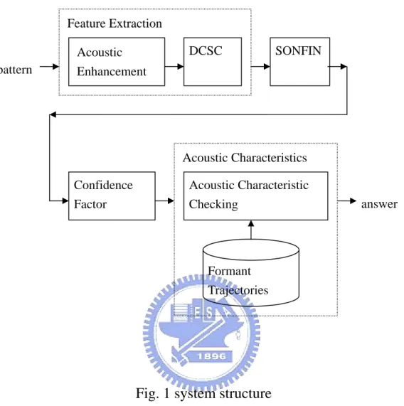
(12) properties of vowels are not always sufficient cues for perception, and that some time-varying information contained in the interval surrounding the vowel “center” is also required. For example, Hillenbrand et al. showed the vowels can be separated with a higher degree of accuracy if spectral change information is included [4]. In this thesis, we tried to search the methods which could effectively solve these problems. There are many published papers in the literature which report phonetic classification and/or recognition results using the TIMIT database. Several well-known and important works are as following: Meng and Zue used the auditory model output and neural networks [21]; Goldenthal and Glass used MFCCs and Gaussian multi-state / spectral trajectories [18]; Gish and Ng used MFCCs, △MFCCs, durations and segmental speech modeling [22]. The best result shown in these published works are the system using DCSCs and partitioned neural networks which was proposed by Zahorian et al [13]; The accuracy rate of the system is 71.50%. In this thesis, a new speaker-independent English vowel recognition system is constructed as shown in Fig. 1. The knowledge about acoustic-phonetic characteristics is taken into consideration and then integrated into the feature representation AE-DCSC which is based on acoustic enhancement and the DCSC encoding process in the procedure of feature extraction. Then the extracted speech feature set is employed to train a fuzzy neural network SONFIN [14]. Finally, the recognition result from SONFIN is checked by a procedure of acoustic-checking to decide the final result. 5.
(13) Feature Extraction. pattern. Acoustic Enhancement. DCSC. SONFIN. Acoustic Characteristics Confidence Factor. Acoustic Characteristic Checking. answer. Formant Trajectories. Fig. 1 system structure. This thesis is organized as follows. In chapter 2, the proposed recognition system, including acoustic-enhanced feature sets, neural fuzzy inference network, and the acoustic-checking process, will be interpreted. In chapter 3, we will verify the performance of the proposed vowel recognition system. The results of experiments were shown in order to show the superior ability of the system. In chapter 4, the conclusions of our work are summarized.. 6.
(14) Chapter 2 Framework of the Acoustic-Phonetics and SONFIN. Based. Speaker-Independent. English Vowel Recognition System 2.1 Introduction As mentioned in Chapter 1, we know that both the acoustic characteristics and the gross shape of the smoothed spectral envelope used to distinguish the vowels have their own advantages and drawbacks respectively. Therefore, we propose a novel system which integrates both the mentioned feature sets and puts them in the suitable position as shown in Fig. 1. The details of the system will be described in this chapter. There are two major components in the proposed system. The first one used the gross shape of the smoothed spectral envelope to extract a set of time-frequency features which give more basic distinguished information about vowels. In this phase, some skills called as “acoustic enhancement” are adopted, in order to enhance the representation ability of the spectrum. Once the feature set was extracted, an on-line self-constructing neural fuzzy inference network (SONFIN) is chosen as the main classifier in our recognition system. The SONFIN is designed to give a score to each candidate. Form these scores, then the so-called confidence-factor which reflected the amount of difficulty in arriving at a decision is estimated. If the value of confidence-factor is too low (i.e. the classification result of SONFIN is not confide in enough), an acoustic 7.
(15) knowledge based sub-system plays a complementary role in choosing the more reasonable and possible result. The proposed sub-system is called as “acoustic characteristic checking”, because it is designed to check the reasonability of these candidates with higher scores.. 2.2 Acoustic-Enhanced Feature Set It is proved that the features derived from the gross shape of the smoothed spectral envelope perform better than those from acoustic characteristics in the complicated and natural environment. This is because the acoustic features are difficult to be measured accurately, when vowels are spoken by different unlimited talkers, in different phonetic environments, at different speaking rates, at different fundamental frequencies, or with varying levels of contrastive stress. As shown in many acoustic-perception researches, the trajectories should be the most important acoustic evidence for vowel recognition, but it is difficult to represent the trajectory automatically well in the finite feature dimensions. Besides, to automatically extract the formant trajectory is unreliable due to the spurious spectral peaks. Here, we propose a set of gross-shape based features and apply the enhancement of the acoustic representation of the spectrum. This set of features is called as acoustic-enhanced discrete-cosine-series-coefficients (AE-DCSCs).. 8.
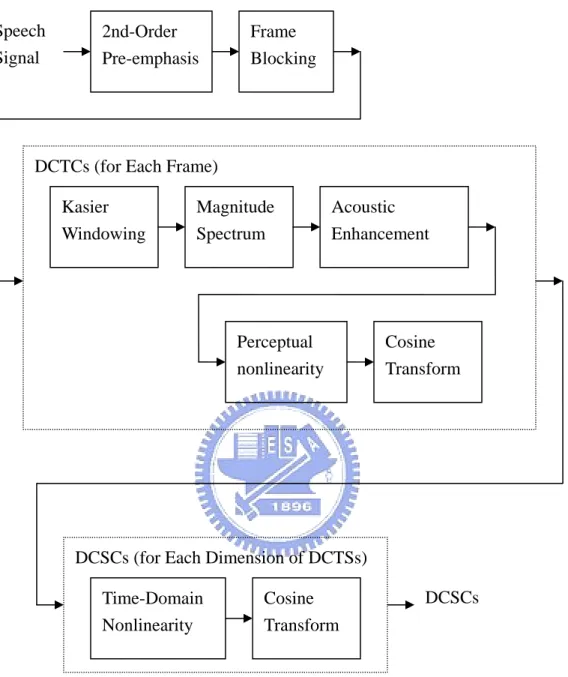
(16) Speech Signal. 2nd-Order Pre-emphasis. Frame Blocking. DCTCs (for Each Frame) Kasier Windowing. Magnitude Spectrum. Acoustic Enhancement. Perceptual nonlinearity. Cosine Transform. DCSCs (for Each Dimension of DCTSs) Time-Domain Nonlinearity. Cosine Transform. DCSCs. Fig. 2 procedure of feature extraction. 9.
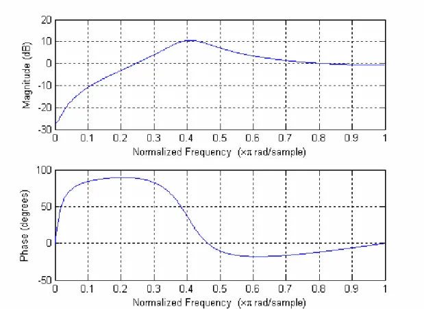
(17) An abstract illustration of the procedure used to extract the feature sets is presented in Fig. 2. The speech signal (16 kHz sampling rate, 16 bit resolution) is first pre-emphasized using the second-order equation. y[n] = x[n] – 0.95x[n - 1] + 0.49y[n - 1] – 0.64y[n - 2].. (2. 1). The frequency response is shown in Fig. 3.. Fig. 3 frequency response of 2nd order pre-emphasis. Observing this plot, we can know that the second-order pre-emphasis has a peak at approximately 3 kHz (0.375π), and therefore is a reasonably good match to the inverse of an equal-loudness contour, results in slightly better performance than does a first order pre-emphasis, (y[n] = x[n] 10.
(18) -0.95x[n-1]) . The next step is to compute the magnitude spectrum of each frame of data with an FFT. Each frame is Kaiser “windowed,” using a coefficient of 5.33 (i.e., approximately a Hamming window). Then, the skills of acoustic enhancement are adopted to improve each traditional FFT according to its acoustic phenomena. The details about acoustic enhancement will be introduced in later sections. The next step in processing is to compute a cosine transform of the scaled magnitude spectrum, but with variations and additions as described later in the chapter to implement the designed frequency and time non-linearity.. The. discrete-cosine-series-coefficients. (DCSCs). are. adopted to represent the encoded movement of spectral shapes according to time. The DCSCs have much better performance due to the ability of scalable frequency-time warping. The more complete investigation about DCSCs will be showed later.. 2.2.1 Acoustic Spectrum Enhancement The features adopted here are derived form the spectrum of the pattern. Therefore, the shape of the spectrum played an important role in representing the identity of this vowel. In this section, we introduce the technique which is use to improve the representation of spectrum. The first skill is the application of broadband spectrum-level normalization (SLN). The motivation behind this step is to reduce as much as possible within-vowel-category differences in formant amplitude relations, following data such as Klatt [26] indicating that formant amplitude variation contributes little to perceived vowel color, while quite audible to 11.
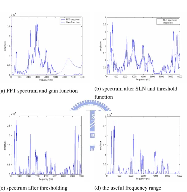
(19) listeners. Therefore, SLN is adopted in order to balance the amplitude of different formants. The idea of the SLN operation, then, is simply to attenuate spectral regions of relatively high amplitude and amplify regions of relatively low amplitude, reducing the magnitude of amplitude differences among broad spectral peaks. The implementation of SLN is done by computing a gain function is relatively low in spectral regions with high average amplitude and, conversely, is relatively high in spectral regions with low average amplitude. The gain function is computed as simply the inverse of the Gaussian-weighted running average of spectral amplitudes computed over an 81-channel (2531.2 Hz) spectral window. Then, the SLN spectrum is obtained from the original spectrum multiplied by the gain function. The original spectrum and its corresponding. gain. function. are. shown. in. Fig.. 4(a).. Here,. Gaussian-weighted running average refers to an approximation implemented with three passes of a rectangular (i.e. un-weighted) running average. Greater weight is assigned to spectral values at the center of the averaging window than to values nearer to the edge of the window. The distribution of weights follows a Gaussian function. Fig. 4(b) shows the spectrum after application of the broadband SLN operation. It can be seen that the variation in spectral peak amplitudes has been considerably reduced, although by no means entirely eliminated. The size of the smoothing window is a compromise, determined by inspecting a large number of individual normalized and un-normalized spectra. The rather large window size that is selected represents a compromise between two competing considerations. Very large window sizes produce rather limited benefit with respect to the goal of minimizing the importance of formant 12.
(20) amplitude differences but have the advantage that they seldom amplify minor spectral peaks that are of little or no perceptual relevance. Smaller window sizes, on the other hand, do an excellent job of reducing the range of formant amplitude variation but can sometimes have the undesirable effect of amplifying minor spectral peaks. Another important skill used is called as enhancement of spectral peak (ESP). The signal processing step consists of a thresholding procedure. The idea here is simply to emphasize the spectral peak regions (both narrow and broad band) that are known to have the greatest influence on vowel identity and to suppress the largely irrelevant spectral components in between harmonic peaks and in the less perceptually significant valleys that lie in between broad spectral peaks. This step is implemented by defining a threshold function as the Gaussian-weighted running average of spectral amplitudes computed over a 21-channel (656.2 Hz) spectral window. The running average is then subtracted from the spectrum, with all negative values (i.e., values below the threshold) set to a small positive value (not zero, to avoid log(0) in the next feature-coding procedure). As with the gain function described above, the size of the averaging window used for the threshold operation is determined through extensive informal experimentation using a vowel database other than the one used to evaluate the model. The process involved examination of a large number of individual cases of spectra with and without the thresholding operation and trying to find a smoothing window size that appeared to do the best job of enhancing the information-bearing aspects of the spectra (i.e., harmonics, especially those defining formant peaks). Only the spectrum within the useful 13.
(21) frequency range is taken into consider in order to eliminate the trivial high band. A frequency range of 75 Hz to 6000 Hz is used, as shown in Fig. 4(d).. (a) FFT spectrum and gain function. (b) spectrum after SLN and threshold function. (c) spectrum after thresholding. (d) the useful frequency range. Fig. 4 signal processing in the acoustic enhancement procedure. 14.
(22) 2.2.2 Discrete-Cosine-Series-Coefficients A powerful encoding method, which is suitable for speech spectra, called as Discrete-Cosine-Series-Coefficients (DCSC) is introduced here. DCSCs successfully encode the trajectories of the perceptual spectra of vowels and represent them in finite dimensional time-frequency features. Some method such as 2D-MFCC also encoded the movement of spectral shapes according to time, but the DCSCs have much better performance due to the ability of scalable frequency-time warping. The suitable parameters for warping are adjusted via pilot experiments. The DCSCs are computed form the static encoding method, Discrete-Cosine-Transform-Coefficients (DCTC), which encoded only the spectrum of each one frame. The procedure to evaluate DCTCs is shown as following. Let X(f ) be the magnitude spectrum represented with linear amplitude and frequency scales and let X’(f’) be the magnitude spectrum as represented with perceptual amplitude and frequency scales. Let the relations between linear frequency and perceptual frequency, and linear amplitude and perceptual amplitude, be given by. f’ = g(f ),. X’ = a(X).. (2. 2). For convenience of notation in later equations, and are also normalized, using an offset and scaling, to the range {0, 1}. The acoustic features for encoding the perceptual spectrum are computed using a cosine transform. 15.
(23) 1. DCTC (i ) = ∫ X ' ( f ' ) cos(πif ' ) df '. (2. 3). 0. where DCTC(i) is the ith feature as computed form a single spectral frame. Making the substitutions. f' = g(f),. X’(f’) = a(X(f)),. (2. 4). and. df ' =. dg df df. (2. 5). the equation can be rewritten as. 1. DCTC (i ) = ∫ a ( X ( f )) cos[π i g ( f )] 0. dg df df. (2. 6). We therefore define modified basis vectors as. φi ( f ) = cos[πig ( f )]. dg df. (2. 7). and re-write the equation as. 16.
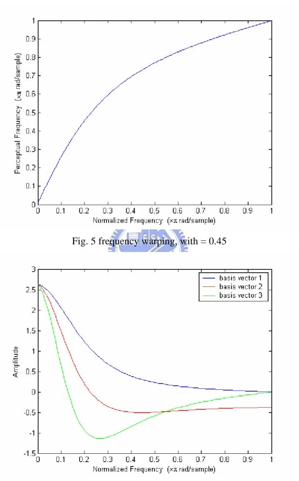
(24) 1. DCTC (i ) = ∫ a ( X ( f ))φ i ( f )df. (2. 8). 0. Thus, using the modified basis vectors, all integrations are with respect to linear frequency. In practice, therefore, the integration of DCTC can be implemented as a sum, directly using spectral magnitude values obtained from our proposed acoustic enhanced spectrum. Any differentiable warping function can be precisely implemented, with no need for the triangular filter-bank typically used to implement warping in MFCC. Except for the frequency warping method and other spectral “preprocessing” refinements as mentioned above, the terms computed with (2. 8) (DCTC(i)) are equivalent to cepstral coefficients. However, to emphasize the underlying cosine basis vectors and the calculation differences relative to most cepstral coefficient computations, we call them the discrete cosine transform coefficients (DCTCs). The suggested DCTC is computed with () using a logarithmic amplitude scale (i.e. a(f ) is the log function) and bilinear warping with a coefficient α = 0.45:. a(f ) = log(f ). g( f ) = f ' = f +. (2. 9). α sin(2πf ) ) tan −1 ( 1 − α cos(2πf ) π 1. (2. 10). Fig.5 and Fig.6 showed the frequency warping function and corresponding basis vectors.. 17.
(25) Fig. 5 frequency warping, with = 0.45. Fig. 6 first three DCTC basis vectors, with = 0.45 18.
(26) Once the DCTCs for each frame are obtained, the DCSC features are computed so as to encode the trajectory of the smoothed short-time spectra, but typically with better temporal resolution in the central region than for the end regions. Using the processing as described for the second feature set, DCTC’s (typically 10 to 15) are computed for equally-spaced frames of data spanning a segment of each token. Each DCTC trajectory is then represented by the coefficients in a modified cosine expansion over the segment interval. The equations for this expansion, which are of the same form as for (2. 2)–(2. 8) above, allow non-uniform time resolution as follows. Let the relation between linear time and “perceptual time” (i.e., with resolution over a segment interval proportional to estimated perceptual importance) be given by. t’ = h(t ).. DCTC’(i, t’) = DCTC(i, t). (2. 11). For convenience, and are again normalized to the range {0, 1}. The spectral feature trajectories are encoded as a cosine transform over time using. 1. DCSC (i, j ) = ∫ DCTC ' (i, t ' ) cos(πjt ' )dt '. (2. 12). 0. The DCSC terms in this equation are thus the new features that represent both spectral and temporal information (“dynamic”) over a speech segment. Making the substitutions. 19.
(27) t' = h(t ),. DCTC’(i, t’) = DCTC(i, t). (2. 13). and. dt ' =. dh dt dt. (2. 14). The equation can be rewritten as. 1. DCSC (i, j ) = ∫ DCTC (i, t ) cos[πjh(t )] 0. dh dt dt. (2. 15). We again define modified basis vectors as. θ j (t ) = cos[πjh(t )]. dh dt. (2. 16). And rewrite the equation as. 1. DCSC (i, j ) = ∫ DCTC (i, t )θ j (t )dt. (2. 17). 0. Using these modified basis vectors, feature trajectories can be represented using the static feature values for each frame, but with varying resolution over a segment consisting of several frames. The terms computed in (2. 17) are referred to as discrete cosine series coefficients (DCSC’s) to 20.
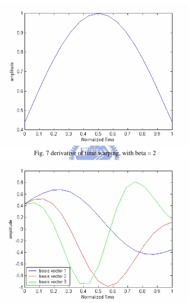
(28) emphasize the underlying cosine basis vectors and to differentiate between expansions over time (DCSC) versus DCTC expansions over frequency. In general, each DCTC is represented by a multi-term DCSC expansion. In our work, the function h(t) is chosen such that its derivative, dh / dt, which determines the resolution for t’, is a Kaiser window, as shown in Fig. 7. Then, the time warping function can be computed from the Kaiser function using numerical method. By varying the Kaiser beta parameter, the resolution could be changed from uniform over the entire interval (beta = 0), to much higher resolution at the center of the interval than the endpoints (beta values of 2 to 15). Fig. 8 depicts the first three DCSC basis vectors, using a coefficient of 2 for the Kaiser warping function. The motivation for these features is to compactly represent both spectral and temporal information useful for vowel classification, with considerable data reduction relative to the original features. For example, 12 DCTC’s computed for each of 50 frames (600 total features) can be reduced to 48 features if four DCSC basis vectors are used for each expansion.. 21.
(29) Fig. 7 derivative of time warping, with beta = 2. Fig. 8 first three DCSC basis vectors, with beta = 2 22.
(30) 2.3 Neural Fuzzy Inference Network The main classifier in our proposed system is a particular fuzzy neural network which is the so-called self-constructing neural fuzzy inference network (SONFIN). The SONFIN is a general connectionist model of a fuzzy logic system, which can find its optimal structure and parameters automatically. There are no rules initially in the SONFIN, and they are created and adapted as on-line learning proceeds via simultaneous structure and parameter learning. The SONFIN can always find itself an economic network size, and the learning speed as well as the modeling ability is all superior to normal neural networks.. 2.3.1 Desired Output The desired output is defined as the membership-value which describes how this pattern belongs to a specified class [29]. Here, a formula to evaluate the membership-value would be given. Let’s consider an l-class problem domain, and there should be also l nodes in the output layer. Let the n-dimensional vectors Ok and Vk denote the mean and standard deviation respectively of the numerical training data for the kth class. A weighted distance could be obtained to represent the normalized distance between this pattern and the class. The weighted distance of the training pattern Fi from the kth class is defined as. ⎡ Fij − okj ⎤ zik = ∑ ⎢ ⎥ v j =1 ⎢ ⎥⎦ kj ⎣ n. 2. (2. 18). 23.
(31) where Fij is the value of the jth component of the ith pattern point, and Ck is the kth class. The weight 1/vkj is used to take care of the variance of the classes so that a feature with higher variance has less weight (significance) in characterizing a class. Note that when all the feature values of a class are the same, then the standard deviation will be zero. In that case, we consider vkj = 1 such that the weighting coefficient becomes 1. this is obvious because any feature occurring with identical magnitudes in all members of a training set is certainly an important feature of the set. Hence its contribution to the membership function should not be reduced. Therefore, the desired output (dk) of the kth output node for the ith input pattern, is defined as. d k = µ k ( Fi ) =. 1 ⎛z 1 + ⎜⎜ ik ⎝ fd. ⎞ ⎟⎟ ⎠. fe. (2. 19). where Fi is the input feature vector, µk(Fi) is the membership value of the ith pattern in class Ck, zik is the weighted distance of the training pattern from and the positive constants fd and fe are the denominational and exponential fuzzy generators controlling the amount of fuzziness in this class-membership set. They influence the amount of overlapping among the output classes. Note that, here we have used a (nonlinguistic) definition of the output nodes which indicates the degree of belongingness of a pattern to a class. However, this definition may be suitably modified in other application areas to include linguistic definitions. Obviously µk (Fi) lies in the interval [0, 1]. Here (2. 19) is 24.
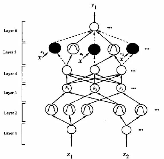
(32) such that the higher the distance of a pattern from a class, the lower its membership value to that class. It is to be noted that when the distance is 0, the membership value is 1 (maximum) and when the distance is infinite, the membership value is 0 (minimum).. 2.3.2 SONFIN The structure of the SONFIN is shown in Fig. 4-2. This 6-layered network realizes a fuzzy model of the following form:. Rule i: IF x1 is Ai1 and … and xn is Ain THEN y is m0i + ajixj + …. (2. 20). where Aij is a fuzzy set, m0i is the center of a symmetric membership function on y, and aji is a consequent parameter. It is noted that unlike the traditional TSK model where all the input variables are used in the output linear equation, only the significant ones are used in the SONFIN; i.e., some ajis in the above fuzzy rules are zero. We shall next describe the functions of the nodes in each of the six layers of the SONFIN. Each node in Layer 1, which corresponds to one input variable, only transmits input values to the next layer directly. Each node in Layer 2 corresponds to one linguistic label (small, large, etc.) of one of the input variables in Layer 1. In other words, the membership value that specifies the degree how an input value belongs to a fuzzy set is calculated in Layer 2. A node in Layer 3 represents one fuzzy logic rule and performs precondition matching of a rule. The number of nodes in layer 4 is equal to that in Layer 3, and the result (firing strength) calculated in Layer 3 is 25.
(33) normalized in this layer. Layer 5 is called the consequent layer. Two types of nodes are used in this layer, and they are denoted as blank and shaded circles in Fig. 9, respectively. The node denoted by a blank circle (blank node) is the essential node representing a fuzzy set of the output variable. The shaded node is generated only when necessary. One of the inputs to a shaded node is the output delivered from Layer 4, and the other possible inputs (terms) are the selected significant input variables from Layer 1. Combining these two types of nodes in Layer 5, we obtain the whole function performed by this layer as the linear equation on the THEN part of the fuzzy logic rule in (2. 20). Each node in Layer 6 corresponds to one output variable. The node integrates all the actions recommended by Layer 5 and acts as a defuzzifier to produce the final inferred output. Two types of learning, structure and parameter learning are used concurrently for constructing the SONFIN. The structure learning includes both the precondition and consequent structure identification of a fuzzy if-then rule. For the parameter learning, based upon supervised learning algorithms, the parameters of the linear equations in the consequent parts are adjusted to minimize a given cost function. The SONFIN can be used for normal operation at any time during the learning process without repeated training on the input-output patterns when on-line operation is required. There are no rules in the SONFIN initially, and they are created dynamically as learning proceeds upon receiving on-line incoming training data by performing the following learning processes simultaneously,. (A) Input/output space partitioning, 26.
(34) (B) Construction of fuzzy rules, (C) Optimal consequent structure identification, (D) Parameter identification.. Processes A, B, and C belong to the structure learning phase and process D belongs to the parameter learning phase.. Fig. 9 network structure of SONFIN. 27.
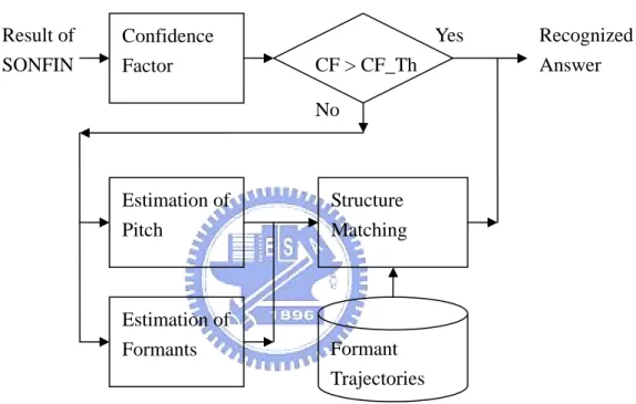
(35) 2.4 Acoustic Characteristic Checking The feature set AE-DCSCs used above successfully encoded the gross shape of spectra. However, some features derived form the acoustic correlates of vowel perception, which play the complementary part, are introduces here. Those feature works when the recognition-result form SONFIN is ambiguous. The most dominant acoustic characteristics are the frequencies of the first three formants (i.e. F1, F2, and F3) and their trajectories. Moreover, it is also found in numerous researches that the gender of the speaker affected the formant trajectories (i.e. the trajectories of the same vowel spoken by men and women are different). Thus, the fundamental frequency (i.e. F0, also called pitch) also played an important role to indicate the gender of the speaker. Numerous pitch determination algorithms (PDA) have been proposed in the past. The most common errors are pitch doubling and pitch having. One of the reasons for pitch doubling and pitch halving is the appearance of alternate pulse cycles in speech signal, which reflects the short-term instability. of. the. vocal. fold. system.. A. PDA. based. Subharmonic-to-Harmonic Ratio (SHR) is adopted here to evaluate the fundamental frequency. Estimation of formant frequencies is generally more difficult than estimation of fundamental frequency. The problem is that formant frequencies are properties of the vocal tract system and need to be inferred from the speech signal rather than just measured. The spectral shape of the vocal tract excitation strongly influences the observed 28.
(36) spectral envelope, such that we cannot guarantee that all vocal tract resonances will cause peaks in the observed spectral envelope, and nor that all peaks in the spectral envelope are caused by vocal tract resonances. Frequently a vital problem of spurious formant arises in the automatic formant estimation system.. Result of SONFIN. Yes. Confidence Factor. CF > CF_Th. Recognized Answer. No. Estimation of Pitch. Structure Matching. Estimation of Formants. Formant Trajectories. Fig. 10 procedure for acoustic checking. Therefore, to avoid the fatal trouble happening in our system, we adopt a strategy, as shown in Fig. 10, in which the formant candidates generated from formant estimation algorithm are just preserved (i.e. all the possible peaks in the spectrum are kept and not assigned as F1, F2, or F3). Then, these candidates are mapped to the formant structure of a specific vowel and it is checked if they are matched. In the proposed system, only the two categories of vowel with the first two higher scores 29.
(37) are mapped to. If there is only one vowel structure matched, the one would be the final recognized result. If none or both are matched, the recognition result form SONFIN would not be changed. Those algorithms about the estimation of confidence factor, the evaluation of pitch and formants, and the construction of formant structure models will be introduced in detail later.. 2.4.1 Confidence Factor We use a measure which reflects the amount of difficulty in arriving at a decision by minimizing the ambiguity in the computed output vector from SONFIN [29]. A confidence factor (CF) is defined as. ⎤ 1⎡ 1 l − CF = ⎢{ ymax } f max + { y y } ∑ max i ⎥ 2⎣ l − 1 j =1 ⎦. (2. 21). where ymax = maxjl=1 {yj}, yj is the jth component in the output vector y, and fmax indicates the number of occurrences of ymax in y. Note that CF take care of the fact that the difficulty in assigning a particular pattern class depends not only on the highest entry in the output vector ymax but also on its differences from the other entries yj. It is seen that the higher the value of CF, the lower is the difficulty in deciding a class and hence greater is the degree of certainty of the output decision. Based on the value of CF, there are two decisions while generating the consequent clause (then part) of the rule. Let yk = ymax such that the pattern under consideration belongs to class Ck. The first one is that the pattern is very likely class Ck, and there is no second choice, if CFk is greater than the 30.
(38) threshold of CF. The second is that the pattern is likely class Ck, and there is second choice, if CFk is less than the threshold. In other words, the recognized result is taken as ambiguous when the confidence factor is not greater than the threshold. In the proposed system, these ambiguous cases will be verified by acoustic checking procedure.. 2.4.2 Acoustic Measurement In this section, we explain the signal processing techniques used in computing the two sets of acoustic characteristics. These two acoustic sets are fundamental frequency and formants.. Fundamental Frequency The general problem of fundamental frequency estimation is to take a portion. of. signal. and. to. find. the. dominant. frequency. of. repetition. Difficulties arise from (1) that not all signals are periodic, (2) those that are periodic may be changing in fundamental frequency over the time of interest, (3) signals may be contaminated with noise, even with periodic signals of other fundamental frequencies, (4) signals that are periodic with interval T are also periodic with interval 2T, 3T etc, so we need to find the smallest periodic interval or the highest fundamental frequency; and (5) even signals of constant fundamental frequency may be changing in other ways over the interval of interest. A PDA based Subharmonic-to-Harmonic Ratio (SHR) which can reduce these problems is adopted to evaluate the fundamental frequency [30]. The SHR-based PDA algorithm is computed in the frequency domain. 31.
(39) First, Let A(f) denote the short-term spectrum function, which is obtained by applying the Fourier transform on windowed short-term speech frames. The length of FFT is varied with the sampling rate and frame length. Suppose that the fundamental frequency is f0, and then the sum of harmonic amplitude is defined as:. N. SH = ∑ A( nf 0 ). (2. 22). n =1. where N is the maximum number of harmonics considered. If we only consider the sub-harmonic frequency that is at one half of fundamental frequency, the sum of sub-harmonic amplitude is defined as:. N. 1 SS = ∑ A(( n − ) f 0 ) 2 n =1. (2. 23). Consequently, SHR can be obtained by dividing SS with SH:. SH =. SS SH. (2. 24). In order to get SS and SH, we could use the direct spectrum compression technique on linear frequency scale as that in Harmonic Product Spectrum (HPS) algorithm. However, because of the numerical problem, a logarithmic transformation on the frequency scale is more preferable, which has been used in Sub-harmonic Summation algorithm (SHS). In 32.
(40) developing the current algorithm, we adopted this basic approach. Nevertheless, the rationale and detail implementation are quite different, which affects the performance in a significant way. To facilitate our work in log domain, we reformulate the above definitions. Let LOGA(f) denote the short-term log spectrum, and log(f0) denote fundamental frequency on the log scale. Therefore, we have:. N. SH = ∑ LOGA(log n + log f 0 ) n =1. (2. 25). N. 1 SS = ∑ LOGA(log(n − ) + log f 0 ) 2 n =1. (2. 26). The log frequency scale is then linearly interpolated. In order to obtain SH, the spectrum is shifted leftward along the logarithmic frequency abscissa at even orders, i.e., log(2), log(4),… log(2N). These shifted spectra are added together.. N. SUMA(log f )even = ∑ LOGA(log f + log(2n)) n −1. (2. 27). From (2. 27), SH is given by:. SH = SUMA(log(0.5 f 0 )) even. Similarly, by shifting the spectrum leftward at log(1), log(3), 33. (2. 28).
(41) log(5), …. log(2N-1), we get SS also at log(0.5f0). N. SUMA(log f ) odd = ∑ LOGA(log f + log(2n − 1)). (2. 29). SS = SUMA(log(0.5 f 0 )) odd. (2. 30). n −1. Next, we obtain the difference function, which is defined as:. DA(log f ) = SUMA(log f )even – SUMA(log f )odd. (2. 31). In so doing, we remove the effect of the contribution of the points around the real peaks, which is equivalent to peak enhancement. Moreover, there are some very interesting properties of the DA(•) function. In ideal cases, if sub-harmonics do not exist, and ignoring the contribution from the points that are at log(nf ) ± log(0.25f0), we would have two maximum values at log(0.5f0) and log(0.25f0) from (2.31), respectively. The values are:. DA(log(0.5f0)) = SH – SS DA(log(0.25f0)) = SH + SS. (2. 32) (2. 33). Therefore, SHR can be approximated by the following simple formula:. SHR = 0.5. DA(log(0.25 f 0 ) − DA(log(0.5 f 0 )) DA(log(log( 0.25 f 0 )) + DA(log(0.5 f 0 )) (2. 34). 34.
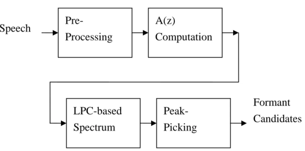
(42) Based on the above analysis, we perform the following procedures to compute SHR and then determine the pitch: First, we locate the position of the global maximum denoted as log f1. Then, starting from this point, the position of the next local maximum denoted as log f2 is selected in the range of [log(1.75f1), log(2.25f1)]. Following (2. 34), SHR can be easily derived:. SHR = 0.5. DA(log( f 1 ) − DA(log( f 2 )) DA(log(log( f 1 )) + DA(log( f 2 )). (2. 35). If SHR is less than a certain threshold value, which is 0.6 in the current implementation, f2 is chosen as the final pitch. Otherwise, f1 will be selected.. Formant Frequency The algorithm adopted in the system to evaluate the formant candidates is based on so-called linear prediction analysis (LP). As shown in Fig. 11, each frame of speech to be analyzed is first preprocessed by pre-emphasis and Hamming windowing. The preprocessed speech is used to design the inverse filter A(z). Then, the LPC-based spectrum is evaluated from 1 / A(z). We chose the peaks in the spectrum as the formant candidates.. 35.
(43) PreProcessing. Speech. A(z) Computation. LPC-based Spectrum. PeakPicking. Formant Candidates. Fig. 11 procedure for formant estimation using linear prediction. The linear prediction analysis is based on modelling the speech signal as if it are generated by a particular kind of source and filter, as shown below.. Fundamental Frequency. Impulse Train Generator u(n). Random Noise Generator. Time-Varying Digital Filter. Lip Radiation Model. G. Fig. 12 simplified model for speech production. 36. s(n).
(44) In this model, the composite spectrum effects of radiation, vocal tract and glottal excitation are represented by a time-varying digital filter whose steady state system function is of the form. H ( z) =. S ( z) G = U ( z ) A( z ). (2. 36). The system can be excited by an impulse train for voiced speech or a random sequence of unvoiced speech. The pitch period and voiced/unvoiced parameters can be estimated using linear predictive analysis. The speech samples s(n) can be given by using simple difference equation. p. s ( n) = ∑ a k • s ( n − k ) + G • u ( n). (2. 37). k =1. The linear predictor with predictor coefficient αk, and order p is defined as a system whose output is. p. s ( n) = ∑ a k • s ( n − k ). (2. 38). k =1. The system function of this linear predictor is. p. p ( z ) = ∑ ak • z −k. (2. 39). k =1. 37.
(45) The prediction error is defined as. e( n ) = s ( n ) − ~ s ( n). (2. 40). Thus the prediction error filter is the output of the system whose transfer function is. p. A( z ) = 1 − ∑α k z − k. (2. 41). k =1. Comparison of (2. 37) and (2. 40) suggests that if αk = ak, then e(n) = G*u(n) and in such condition, prediction error filter A(z) will be an inverse filter for the system H(z). H ( z) =. G A( z ). (2. 42). The basic problem of linear prediction here is to determine a set of predictor coefficients {αk} directly from speech signal in such a manner as to obtain a good estimate of spectral properties of speech signal through the use of (2. 42). The predictor coefficients could be computed efficiently using the Levinson-Durbin recursion [1].. 38.
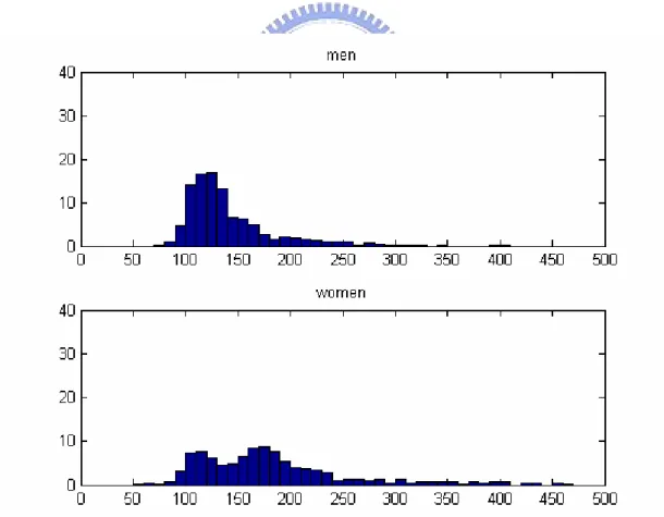
(46) 2.4.3 Modelling Acoustic Characteristics Here, we will introduce the way to construct the formant trajectory model of each model. We used the histogram analysis to analyze these acoustic characterises. The speech database which provides the corpus for analysis is the training set of TIMIT database. The detailed interpretation of TIMIT will be seen in the next chapter. First we used the SHR-based PDA to reveal the relationship between fundamental frequency and the gender of speaker. The threshold of SHR is chosen as 0.6. Fig. 13 showed the distribution of fundamental frequency respectively for men and women.. Fig. 13 the distribution of F0 for men and women. 39.
(47) Form the analysis, a threshold-value of 140 (Hz) is chosen. The patterns whose fundamental frequency is above the threshold are taken as men-like category, and those else taken as women-like category. Then we constructed the trajectory model for each vowel class respectively for both men-like and women-like category. The models are derived the histogram analysis form individual vowel category and consisted of three time-dependent sub-model sampled at 20%, 50% and 80% of the vowel duration. In each sub-model, we chose the pass-bands for F1 and F2 respectively which indicate the formant candidates may be allowed to take place in the frequency range. On the other hand, the stop-band is chosen which prohibited the occurrence of formant candidates in this vowel category. Let’s take the vowel /iy/ of men-like category as an example. In sub-model 1, the pass-band for F1 is chosen as 400~500 Hz, the pass-band for F2 is chosen as 1600~2500 Hz, and the stop-band as 700~1200 Hz. An illustration of the model of a specific vowel category is shown below.. Fig. 14 model of /iy/. 40.
(48) Many acoustic evidences could be found in these models. For example, as shown in Fig. 15, the difference between /iy/ and /ih/ is presented by the location of pass-band and stop-band. In Fig. 16, we could see the temporal trajectories of the diphthongs /ay/ and /oy/. Those phenomena are the cues for the acoustic characteristic checking.. Fig. 15 an illustration of /iy/ and /ih/. Fig. 16 an illustration of /ay/ and /oy/. 41.
(49) Chapter 3 Experiments. 3.1 Introduction In the previous chapter, we described the structures of the proposed vowel recognition system in detail. In order to investigate and show the contribution and correlation of these different techniques we applied, several sets of experiments are done. In the first set of experiments, the method of narrow band pattern-matching model proposed by Hillenbrand [5] was evaluated. The second set of experiments is designed and implemented with DCSCs as feature set and SONFIN as the classifier. In these experiments, we tried to show the superior ability of the neural fuzzy inference network for this classification task. In the third set of experiments, we adopted the AE-DCSCs as the feature set and SONFIN again as the classifier. The improvement caused by the feature enhancement techniques are shown here. Finally, in the last set of experiments, acoustic-checking technique is applied to this system. The experiment results showed the contribution of this process. For these experiments (except for the pattern-matching model), the following 101 features are first computed for each token. The first 45 features encoded 15 DCTC trajectories over 100 ms centered at each vowel midpoint (20-ms frame length, 5-ms frame spacing, 15 DCTCs using three DCSCs, with a warping factor of two). This part of features tried to represent the steady-state of the token (i.e. the duration of vowel 42.
(50) is greater than 100ms). The next 56 features encoded eight DCTC trajectories over 300 ms centered at each vowel midpoint (10-ms frame length, 2.5 ms frame spacing, eight DCTCs using seven DCSCs, with a time warping of 4). This part of features tried to represent the co-articulation phenomenon of the vowel token (i.e. the duration of vowel is less than 300ms and the preceding and following consonants will be included). Thus, these features include varying degrees of time-frequency resolution, based on the conjecture that different vowel pairs might be best discriminated with features varying with respect to these resolutions.. 3.2 Experiment Database The TIMIT acoustic-phonetic speech corpus is used for all training, development, and performance evaluation experiments. This corpus is widely used throughout the world and provides a standard that permits direct comparison of experimental results obtained by different methodologies. The entire corpus consists of 10 sentences recorded from each of 630 speakers of American English. Two of the sentences (sa) are identical for all the speakers. Five of the sentences (sx) for each speaker are drawn from a set of 450 phonetically compact sentences hand-designed at MIT. The emphasis behind these sentences is on covering a wide range of phonetic pairs. The 450 (sx) sentences are each spoken by seven different speakers. The final three sentences (si) for each speaker are chosen at random from the Brown Corpus and are unique for all the speakers. The speakers in the corpus are comprised of males and females (at a ratio of roughly two to one) from eight predefined dialect 43.
(51) regions of the United States. For all experiments, the data is divided into distinct units known as the training set and the test set. The training set is used to estimate the parameters for each of the phonetic models to be used in the experiments. The test set consists of the actual test data for the classification or recognition performance evaluation. Speakers from the training and test sets never overlap. This is important to ensure fair experimental conditions. Both sets are generally chosen to reflect a well balanced representation of the speakers in the corpus. Most of the training and test sets utilized in this work are selected specifically because they are identical to training and test sets used in other work. Therefore, the results can be directly compared to those obtained and reported in the literature. The sets used in this thesis are listed along with some of their statistics in Table 1. The experiments are performed with vowels extracted from the TIMIT database. A total of 16 vowels are used, encompassing 13 monophthongal vowels /iy/, /ih/, /eh/, /ey/, /ae/, /aa/, /ah/, /ao/, /ow/, /uh/, /ux/, /er/, /uw/, and diphthongs /ay/, /oy/, /aw/.. Table 1 data set used for the experiments Data Set. Training Speakers. Test Speakers. Training Tokens. Test Tokens. SX. 450. 50. 17040. 1786. 44.
(52) 3.3 Experiment Result Experiment Set I In this set of experiments, the narrow band pattern-matching model proposed by Hillenbrand [5] was evaluated in the TIMIT database. Hillenbrand summarized the cues from the researches about human vowel perception and proposed the pattern-matching model algorithm. It was assumed that the human perception mechanism is a narrow band pattern-matching procedure. Thus several experiments done by Hillenbrand were used to verify the assumption. The original corpus in those experiments is the database recorded by Hillenbrand et al. it consisted of 1668 /hVd/ utterances spoken by 139 well-trained speakers. The original accuracy rate by Hillenbrand was 91.4%. However in the experiment set I, we used the TIMIT database and the accuracy rate was 32.06%, which was much lower as expected.. Experiment Set II In this set of experiments, we used DCSCs as the feature set and SONFIN as the classifier. Several parameters of SONFIN are adjusted to allow SONFIN to find its optimal structure by itself. There are 21 rules in the best structure of SONFIN. The recognition rate of this structure is 72.72% which is higher than other methodology in the literature (including the 71.50% reached by the system proposed by Zahorian et al.).. 45.
(53) Experiment set III The acoustic enhanced features AE-DCSCs are adopted in experiment set III in order to evaluate the improvement of the feature modification. Again, the neural fuzzy classifier SONFIN is used as the classifier and the parameters of SONFIN are adjusted. There are 14 rules in the best structure of SONFIN for AE-DCSCs. The recognition rate of this structure is 74.41% which is higher than those in experiment set II.. Experiment IV Finally, the acoustic-checking procedure is applied to the result of AE-DCSCs and SONFIN structure. The threshold of confidence factor is chosen as 0.4. and the experiment result showed a recognition rate of 74.75%. Table 2 experiment results and comparison Feature set. Method. Accuracy. Narrow-Band Spectra. Pattern-Matching. 32.06%. Model DCSCs. Partitioned. Neural 71.50%. Networks DCSCs. SONFIN. 72.72%. Acoustic-Enhanced-DCSCs SONFIN. 74.47%. Acoustic-Enhanced-DCSCs SONFIN. + 74.75%. Acoustic Checking 46.
(54) 3.3 Discussion It is shown by these experiments that our proposed system and the applied techniques performed better than those by others in the literature. In the first set of experiments, we showed the poorness of the feasibility in the perception model by Hillenbrand. In the second set of experiments, we just tried to evaluate the classification ability of the neural fuzzy classifier SONFIN if we compare it to the system proposed by Zahorian (1999) [13] which also used the DCSCs as the feature set but partitioned neural networks as the classifier. The experiment showed the accuracy rate by SONFIN is 72.72% higher than the accuracy rate of 71.50 % from the system proposed by Zahorain. Almost 1.2% improved by SONFIN. The experiment results showed the powerful classification ability of SONFIN. It used a simpler structure and easier to be trained than the PNN, but performed better. The reasons may be the partition ability in the input/output space and the effective inference of rules. Each rule constructed in SONFIN may classify the output space as many parts as the output class, and multiple rules are integrated via fuzzy inference which partitioned the output space carefully and precisely. The modified feature set is proved more representative in experiment set III, the higher recognition rate in experiment set II is 74.41% which is 1.69% higher than that in experiment set II. the experiment result showed the idea of the enhancement of the acoustic characteristics in the spectrum domain is feasible. The procedure of acoustic-enhancement emphasized the spectral harmonics and balanced them which suggested in the acoustic-phonetic researches [5]. The acoustic-checking procedure is 47.
(55) applied in experiment IV. The experiment result showed the recognition rate is raised to 74.75%. Thus, the potential and effectiveness of the proposed system was verified.. 48.
(56) Chapter 4 Conclusion. In this thesis, we attempt to develop a more robust speaker independent automatic recognizer for English vowels. We integrate the spectral shape based features and acoustic characteristics in our system. Moreover several techniques are applied in this work. Fist of all, we modify the gross shape of spectrum, which will be encoded to the feature set of the token. In this phase, we try to enhance the spectral peaks by eliminating the variation between harmonics and balance the amplitude difference by a spectrum-level-normalization process. The DCTC is adopted to encode the spectrum with a nonlinearity frequency warping according to the characteristic of human perception. In order to represent the temporal cues, we use the DCSC to encode the trajectory of spectrum. The suitable time warping can be adjusted to preserve the information better in a finite feature dimension. A neural fuzzy inference classifier called as SONFIN is adopted in the proposed system as the main recognizer. The SONFIN has the ability to construct its optimal structure by itself and can self-adjust its parameters such as membership function and the consequent parameters. Experiments showed the SONFIN has a simpler structure and better performance. Finally a formant checking procedure is done in the system. The procedure is used to distinguish the ambiguous cases according to their 49.
(57) acoustic evidence. If the confidence factor form SONFIN classification is not high enough, the recognition-result is taken as ambiguous and their acoustic cues such as fundament frequency and formant trajectory will be evaluated and checked with the model of vowels. This procedure provides another view to look at the token and provide a more accuracy recognition. result.. Many. experiments. based. on. the. popular. acoustic-phonetic database are done and the results showed that our proposed system performed much better.. 50.
(58) Bibliography. [1] L. Rabiner and B. H. Juang, “Fundamentals of Speech Recogntion”, Prentice-Hall International, NJ, 1993 [2] A. M. A. Ali, J. van der Spiegel, and P. Mueller, “Acoustic-Phonetic Fetaures for the Automatic Classification of Stop-Consonants”, IEEE Trans. Speech and Audio Processing, vol. 9, pp. 833-841, 2001. [3] G. Peterson and H. L. Barney, ‘‘Control methods used in a study of the vowels,’’ J. Acoust. Soc. Am. 24, 175–184, 1952. [4] J. Hillenbrand, L. A. Getty, M. J. Clark, and K. Wheeler, ‘‘Acoustic characteristics of American English vowels,’’ J. Acoust. Soc. Am. 97, 3099–3111, 1995. [5] J. Hillenbrand, and A. H. Robert, “A narrow band pattern-matching model of vowel perception”, J. Acoust. Soc. Am 113(2), 1044-1055, 2003. [6] L. C. W. Pols, L. J. van der Kamp, and, R. Plomp, ‘‘Perceptual and physical space of vowel sounds,’’ J. Acoust. Soc. Am. 46, 458–467, 1969. [7] Z. B. Nossair and S. A. Zahorian, “Dynamic spectral shape features as acoustic correlates for initial stop consonants,” J. Acoust. Soc. Amer., vol. 89, pp. 2978–2991, 1991. [8] Z. B. Nossair, P. L. Silsbee, and S. A. Zahorian, “Signal modeling enhancements. for. automatic. ICASSP’95, pp. 824–827. 51. speech. recognition,”. in. Proc..
(59) [9] L. Rudasi and S. A. Zahorian, “Text-independent talker identification with neural networks,” in Proc. ICASSP’91, pp. 389–392. [10] L. Rudasi and S. A. Zahorian, “Text-independent speaker identification using binary-pair partitioned neural networks,” in Proc. IJCNN’92, pp. IV: 679–684. [11] S. A. Zahorian and A. J. Jagharghi, “Spectral-shape features versus formants as acoustic correlates for vowels,” J. Acoust. Soc. Amer., vol. 94, pp. 1966–1982, 1993. [12] S. A. Zahorian, D. Qian, and A. J. Jagharghi, “Acoustic-phonetic transformations for improved speaker-independent isolated word recognition,” in Proc. ICASSP’91, pp. 561–564. [13] S. A. Zahorian and Z. B. Nossair, “A partitioned neural network approach for vowel classification using smoothed time/frequency features”, IEEE Trans. Speech and Audio Processing, vol. 7, pp. 414-425, 1999. [14] C. F. Juang and C. T. Lin, “An on-line self-constructing neural fuzzy inference network and its application,” IEEE Trans. Fuzzy Syst., vol. 6, pp. 12–32, 1998. [15] C. T. Lin and C. S. G. Lee, Neural Fuzzy Systems: A Neural-Fuzzy Synergism. to. Intelligent. Systems.. Englewood. Cliffs,. NJ:. Prentice-Hall, 1996. [16] C. T. Lin, Neural Fuzzy Control Systems with Structure and Parameter Learning. Singapore: World Scientific, 1994. [17] W. D. Goldenthal, “Statistical trajectory models for phonetic recognition,” Ph.D. dissertation, Mass. Inst. Technol., Cambridge, Sept. 1994. 52.
(60) [18] W. D. Goldenthal and J. R. Glass, “Modeling spectral dynamics for vowel classification,” in Proc. EUROSPEECH’93, pp. 289–292. [19] H. Leung and V. Zue, “Some phonetic recognition experiments sing artificial neural nets,” in Proc. ICASSP’88, pp. I: 422–425. [20] H. Leung and V. Zue, “Phonetic classification using multi-layer perceptrons,” in Proc. ICASSP’90, pp. I: 525–528. [21] H. M. Meng and V. Zue, “Signal representations for phonetic classifi-cation,” in Proc. ICASSP’91, pp. 285–288. [22] H. Gish and K. Ng, “A segmental speech model with applications to word spotting,” in Proc. ICASSP’93, pp. II-447–II-450. [23] M. S. Phillips, “Speaker independent classification of vowels and diphthongs in continuous speech,” in Proc. 11th Int. Cong. Phonetic Sciences, 1987, vol. 5, pp. 240–243. [24] R. A. Cole and Y. K. Muthusamy, “Perceptual studies on vowels excised from continuous speech,” in Proc. ICSLP’92, pp. 1091–1094. [25] B. S. Rosner and J. B. Pickering, “Vowel Perception and Production”, Oxford U.P., Oxford, 1994 [26] D. H. Klatt, ‘‘Prediction of perceived phonetic distance from critical-band spectra: A first step,’’ IEEE ICASSP, 1278–1281, 1982. [27]S. K. Pal and S. Mitra, “Multilayer perceptron, fuzzy sets, and classifi-cation,” IEEE Trans. Neural Networks, vol. 3, pp. 683–697, 1992. [28] S. Mitra and S. K. Pal, “Fuzzy multilayer perceptron, inferencing and rule generation,” IEEE Trans. Neural Networks, vol. 6, pp. 51–63, 1995. [29]S. Mitra, R. K. De. and S. K. Pal, "Knowledge-Based Fuzzy MLP for 53.
(61) Classification and Reule Generation," IEEE Trans. Neural Networks, vol. 8, pp. 1338–1350, 1997. [30] X. Sun, "Pitch determination and voice quality analysis using subharmonic-to-harmonic ratio," IEEE ICASSP2002, , 2002, Vol 1, pp 333-336.. 54.
(62)
數據
+7
相關文件
A factorization method for reconstructing an impenetrable obstacle in a homogeneous medium (Helmholtz equation) using the spectral data of the far-field operator was developed
A factorization method for reconstructing an impenetrable obstacle in a homogeneous medium (Helmholtz equation) using the spectral data of the far- eld operator was developed
In this paper, we evaluate whether adaptive penalty selection procedure proposed in Shen and Ye (2002) leads to a consistent model selector or just reduce the overfitting of
Wang, Unique continuation for the elasticity sys- tem and a counterexample for second order elliptic systems, Harmonic Analysis, Partial Differential Equations, Complex Analysis,
Reading Task 6: Genre Structure and Language Features. • Now let’s look at how language features (e.g. sentence patterns) are connected to the structure
Now, nearly all of the current flows through wire S since it has a much lower resistance than the light bulb. The light bulb does not glow because the current flowing through it
volume suppressed mass: (TeV) 2 /M P ∼ 10 −4 eV → mm range can be experimentally tested for any number of extra dimensions - Light U(1) gauge bosons: no derivative couplings. =>
• Formation of massive primordial stars as origin of objects in the early universe. • Supernova explosions might be visible to the most
