E L S E V I E R Pattern Recognition Letters 17 (1996) 467-473
Pattern. Recognition
Letters
A high-speed algorithm for line detection
Chun-Ta Ho, Ling-Hwei Chen *
Department of Computer and Information Science, National Chiao Tung University, Hsinchu 30050, Taiwan, ROC
Received 6 March 1995; revised 7 December 1995
Abstract
A high-speed method for line detection is proposed in this paper. By shifting the black points in a black/white image 1, a parallel line for each straight line on I will be generated. Through the use of the geometric property on a pair of parallel lines, the parameter sets of those lines possibly on I can be obtained immediately. Since the transform from image space to parameter space is one to few points, the proposed method can significantly reduce the number of transforms for evaluating possible parameter sets. Experimental results are also given to show the correctness and effectiveness of the proposed method.
Keywords: Line detection; Parallel lines; Geometric property
1. I n t r o d u c t i o n
Detecting straight lines from an image is one of the basic tasks in computer vision. Hough transform for line extraction is well known and has been widely used (Hough, 1962; Duda and Hart, 1972). The method consists of three basic steps:
(1) transform a feature point in an input image into a curve on parameter space;
(2) each transformed point in parameter space is considered as a candidate and accumulated in the corresponding cell;
(3) a local peak-finding algorithm is applied to extract true parameters. These steps are feasible, but it causes the following two problems:
1. A lot of computing time is needed to transform each feature point in image space into a curve (many points) in parameter space.
* Corresponding author.
2. For one feature point in image space, all possi- ble set of parameters are accumulated in parameter space, but among them, only one set is correct.
Several modified versions of Hough transform have been proposed (Leavers, 1993). Some of them have realized that the computational load can be reduced using the coarse-to-fine accumulation tech- nique (Li et al., 1986; Illingworth and Kittler, 1987; Atiquzzaman, 1992) or the random sampling concept (Xu et al., 1990). These methods try to solve the previously mentioned problems, but they still pro- duce many superfluous points in parameter space. On the other hand, some use the local gradient information to reduce the dimension of lines (O'Gor- man and Clowes, 1976; Davies, 1987), but they often suffer from poor consistency and locating ac- curacy due to noises and quantization errors in digi- tal black/white images. Thus, developing a straight line extracting method, that is fast as well as easily applied to various practical applications, is very im- portant. In the paper, we will present such a method. 0167-8655/96f$12.00 © 1996 Elsevier Science B.V. All rights reserved
468 C.-T. Ho, L.-H. C h e n / Pattern Recognition Letters 17 (1996) 467-473
First, the proposed method shifts each black point in a b l a c k / w h i t e image F with a certain distance. Through the shifting, a parallel line L 2 for each straight line L 1 on F will be generated. Then, for each black point A in F, by the geometric property on a pair of parallel lines, the parameters of those lines possibly passing through A will be obtained. Finally, based on the accumulative concept of Hough transform, each straight line on F will be extracted. Note that in the proposed method, for each black point, only few parameter sets are evaluated, and the local gradient information is not used.
2. T h e p r o p o s e d m e t h o d
For convenience, before describing the proposed method in detail, we will first introduce a definition and theorem, which will be used in the proposed method.
2.1. Definition and theorem
D e f i n i t i o n 1. Let L~ and L 2 be a pair of parallel lines, A ( x o, Yo) be a point on L~. The horizontal buddy point B of A on L 2 is defined to be the point on L 2 with coordinates ( x~, Yo). The vertical buddy
Fig. I. L~ and L 2 are a pair of parallel lines, L 2 is generated by shifting L~ toward right direction w pixels. A is a point on L~, B and C are the horizontal and vertical buddy points of A on L e, respectively.
point C of A on L 2 is defined to be the point on L 2 with coordinates ( x 0, y~) (see Fig. 1).
L e m m a 1. Let L~ be a line, L z be the line f o r m e d by shifting each point on L l toward right direction w pixels. Then L 1 is parallel to L 2.
L e m m a 1 is trivial, so the proof is omitted. Through L e m m a 1, we can derive the following theorem.
T h e o r e m 1. Let L 1 be a line, L 2 be the line f o r m e d by shifting each point on L l toward right direction w pixels. L e t A ( x o , Yo) be a point on L l and C ( x o, Yl) be the vertical buddy point o f A on L 2. Assume that L 1 is expressed as (Duda and Hart, 1972):
p = x cos O + y sin 0, (1) where p is the normal distance f r o m the origin to L l, 0 is the angle between the normal o f L l and the X-axis. Then
0 = tan - l . (2)
Proof. Through L e m m a 1, we can see that L~ is parallel to L 2 . Assume that B is the horizontal buddy point of A on L 2. Then B has coordinates ( x 0 + w, Y0)- Since A C is parallel to the Y-axis, from Fig. l, we can get
Z_ N P O = Z_ CAP =/__ BCA.
Since O M is the norm vector of L l, zx O M N is a right triangle. This leads to
/x O M N ~ zx P O N , and we can further get
0 = / _ N O M =/__ N P O = Z. BCA.
Since / _ B C A = t a n - l ( w ) / ( yl --Yo), this leads to
0 = t a n - ~ . []
2.2. The proposed line detector
In this subsection, we will present the proposed method. Based on Theorem 1, the parameters (0, p) for each straight line on a b l a c k / w h i t e image F will be found. Initially, a two-dimensional array AR with
C.-T. Ho, L.-H. Chen /Pattern Recognition Letters 17 (1996) 467-473 469 AR(0, p ) = 0 for each entry (0, 0) is established.
Next each black point D(x, y) in F is shifted toward right direction w pixels to get D'(x + w, y),
which will form another black/white image F'. Then for each black point A(x o, Yo) in F, each black point C with coordinates ( x 0, y¿) in F' is taken. By substituting ( Y l - Y0) and w into Eq. (2), 0 is first obtained, and then by putting the obtained 0 and ( x 0, Y0) into Eq. (1), we can get 0. The (0, p) are considered to be the parameters of a candidate straight line, and the corresponding entry AR(0, 0) is increased by one. After all black points in F are processed, a local peak-finding algorithm is finally applied to array AR and each found peak is considered to be the parameters of a true straight line.
Note that if there exists a straight line L] with parameters (00, 00), through the proposed method, a parallel line L 2 will be generated. From Theorem 1, we can see that each point A(x o, Yo) on L~ with its vertical buddy point C on L 2 will contribute one to AR(00, 00)- Hence, the value of AR(00, 00) must be large and L l can be found through the local peak-finding algorithm.
2.3. Applying the method to real cases
The proposed method can significantly reduce the number of transforms from image space to parameter space. However, applying the method to real cases still leads to two problems:
1. Noise or non-line black points cause many superfluous transforms.
2. Nearly vertical or horizontal lines can not be detected since correct vertical buddy points can not be located.
Based on the line property that if two points B and C are on a line, then their mid-point must be also on the line, a noise filter is added to treat Problem 1 and is described as follows.
In the proposed method, after A and C are lo- cated, the filter will take the mid-point M ( x m , Ym) of BC as
( w y ° + Y l )
g ( x , , , y,,)= Xo+ 2 ' 2 '
where B is the shifted point of A. Then M is checked to see whether M is a black point in F'. If
yes, point A is considered to be a point lying on a straight line and the corresponding parameter set (0, 0) is computed and accumulated in the accumu- lation array. Otherwise, no more process is done.
On the other hand, in order to treat Problem 2, we apply the proposed method twice. First, the proposed method is applied to extract lines with [ 0 I E [22.5 °- 67.5°], then all black points are rotated clockwise 45 ° relative to the origin, and the proposed method is applied again to obtain lines with
101
E [00-22.5 °] or [67.5°-90°]. The entire proposed method is de- scribed as follows.T h e p r o p o s e d m e t h o d
Step 1. Initialize a blank array AR;
Step 2. Shift F toward right direction w pixels to get another image F';
Step 3. For each black point A(x o, Yo) in F For each black point C(x o, y]) in F' Set M( x m, y,,) to be
( w Y ° + Y ' )
x° + 2 ' 2 " (3)
If M is a black point in F', then
0 = tan- 1 . (4)
If 22.5 ° < l 0 ] < 67.5 °, then
p=Xo cos O+y o sin O; (5)
AR( O, 0) = AR( O, 0) + 1; (6)
Step 4. The black points in F are rotated clockwise 45 ° relative to the origin as a new input image F~; Set F = FI;
Apply Steps 2-3, where Eq. (6) is modified
a s
A R ( O - 45 ° , p) = A R ( 0 - 45 ° , 0) + 1;
Step 5. Apply a peak-finding algorithm to AR;
For each extracted peak (0, 0)
Consider (0, 0) to be the parameters of a true line.
3. T h e c o m p l e x i t y analysis
In this section, we will analyze the computational complexities of the Hough transform and the pro-
4 7 0 C.-T. Ho, L.-H. Chen / Pattern Recognition Letters 17 (1996) 467-473
posed method. For convenience of illustration, some symbols are defined as follows:
q
n
b =
t a
tin----
The number of intervals which span the pa- rameter range when quantized;
the average number of black points on each column;
the average number of candidate buddy points for each black point;
the computation time of one c o m p a r i s o n / s h i f t operation;
the computation time of one addition/subtrac- tion operation;
the computation time of one complex opera- tion ( * , / , sin, cos, atan).
For the Hough transform, each black point is transformed into q sets of (0, p ) through Eq. (1), the computation time needed is
qt a + 2 q t m.
On the other hand, for each black point A and for each black point C on the same column as A in F ' ,
the proposed method uses Eq. (3) to evaluate M and checks M to see if it is a black point, this will cost
3 n t c + 2 n t , . Then, if M is a black point, a set of (0, p ) is generated through Eqs. (4)-(5), this will need time 2 b t a + 4 b t m. Thus, for each black point A, the total computation time is
3 n t c + 2( n + b ) t a -k- 4 b t m.
In practice, for most images (except some full of noise), both n and b are much smaller than q (this conclusion will also be shown in the experimental result, which will be described later), t c and ta are smaller than tm. Thus, the proposed method will be faster than the Hough transform.
Note that in the proposed method, the shifting distance w will affect the preciseness of 0 and determine the minimum length o f a line, which can be detected. The distortion of 0 can be estimated as follows. Let A ( x o, Yo) be a point on a line L l with 0 = 0 o. Let L 2 be the line formed by shifting L, toward right direction w pixels. Then the vertical buddy point C of A on L 2 will have coordinates (Xo, Yl), Yl should be an integer due to digitization. However, the exact value of the y-coordinate of C
should be Yo + ( w / t a n 00), and y, is the nearest integer to Yo + ( w / t a n 00). So, Yl will be
lt&l
Yo + or Yo + ,
and the obtained 0 will be
W W
t a n - 1 or t a n - 1
tw/tan
001
[w/tan
0o1'
the distortion for 0 0, expressed as A0 0, is
= tan - I w [ A 0 o [ w / t a n 0 o ] 0° or W × t a n - ' [ w / t a n 0o] O° ' where I Oo J ~ [22.5°-67.5°]. (7)
On the other hand, the m i n i m u m length of a line L~ with 0 = 00, which can be detected, can be estimated as follows. Let A ( x o, Yo) be a point on line L l, C ( x o, y , ) be the vertical buddy point of A on the shifted line L:. I f C can be found, this means that the point C ' ( x o - w, y , ) is also on line L, and on the input image. Thus the line L, at least contains
2.5 2 1.5 1 0.5 0 (a) I L I i 10 20 30 40 50 140 120 100 80 60 40 20 0 (b) i i I I 0 10 20 30 40 50
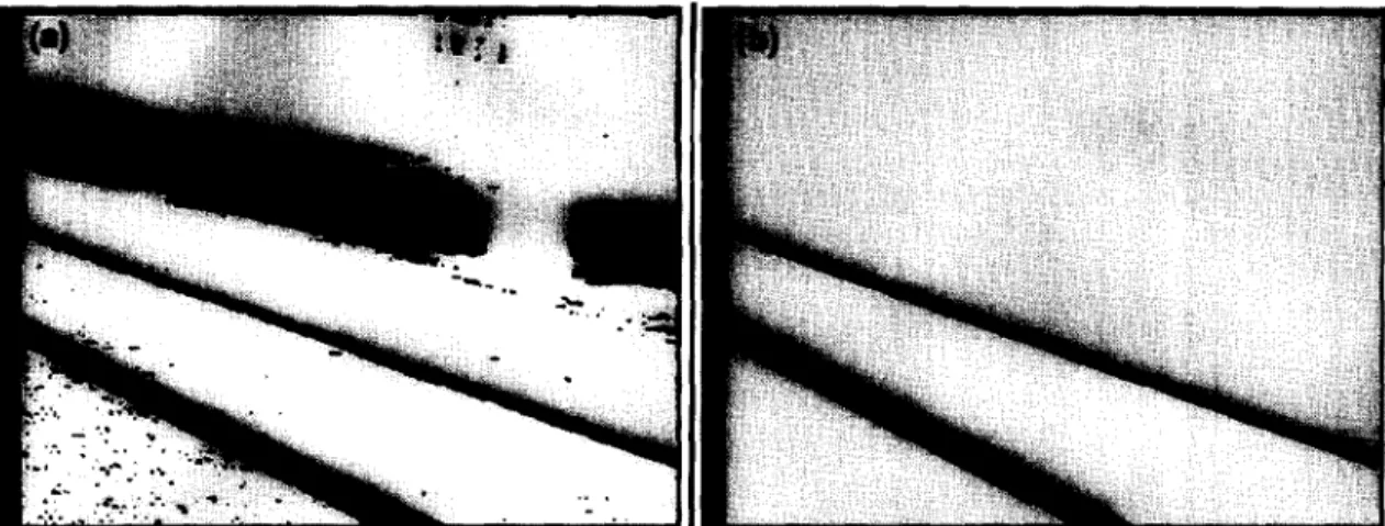
Fig. 2. The relationships of w, A 0,1 and Im. (a) The relationship between w and AOm. (b) The relationship between w and Im.
C.-T. Ho, L.-H. Chen / Pattern Recogn#ion Letters 17 (1996) 467-473 471 line segment A-C. Since Yl -- YO ---- w / t a n - l O0 ' the
length of ~ is about
Thus, to make sure that line L1 can be detected, the minimum length of line L~, expressed as loo, should be larger than
,
where [00 I E [22.5°-67.5°].
Note that in our proposed method, lines with I 0 I ~ [0°-22.5 °] or I 0 1 E [67.50-90 °] are rotated clockwise 45 ° to make 0 lie within [22.5°-67.5°]. Thus, for a line with such a 0, the distortion A 0 and
the minimum line length can also be evaluated through F_zlS. (7)-(8). Define A0 m = max o A0, l m = m a x o l o. Fig. 2 shows the relationships between w and A 0 m and between w and l m, respectively. Refer- ring to this figure, we can decide w based on the detecting minimum length and precision needed. In our experiment, for a 5 1 2 . 5 1 2 image, we take w = 30.
4. Experimental results
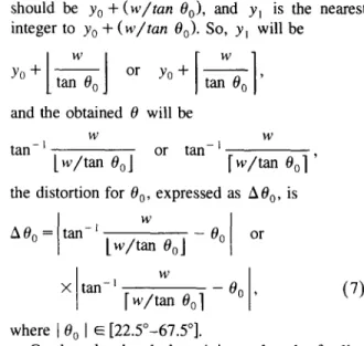
This section will present two experimental results of applying the proposed method to a 512 × 512 real and a synthetic image. Fig. 3(a) is an image caught from an automatic land vehicle led by road-lines. Fig. 3(b) is the edge image of Fig. 3(a). Fig. 3(c)
Fig. 3. The experimental result of applying the proposed line detector. (a) A real image. (b) The edge image of (a). (c) The detection result of applying the proposed method to (b); four straight lines are detected.
472 C.-T. Ho, L.-H. Chen / Pattern Recognition Letters 17 (1996) 467-473
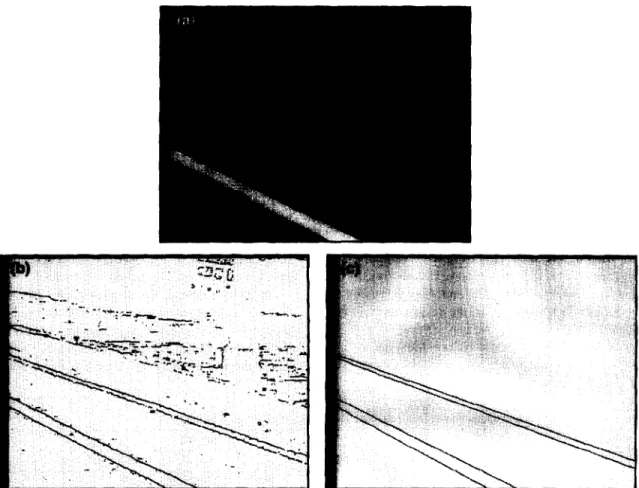
Fig. 4. The experimental result of applying the proposed method to a synthetic image. (a) A machine-part drawing. (b) The detection result superimposed on (a).
shows the detection result of applying the proposed method to Fig. 3(b) with shifting distance w = 30, four straight lines are detected. From this figure, we can see that the proposed method works well. Fig. 4 shows the experimental result of applying the pro- posed method to a machine-part drawing. From the detection result, we can see that most straight lines have been detected, only a few shorter lines have not. This is due to that a detected line must satisfy the following two conditions: (1) the length of the line must exceed the minimum length mentioned in Section 3; (2) the line must consist of enough points to get correct line parameters and to accumulate them in parameter space to form a peak. If a line cannot satisfy the above two conditions, the pro- posed method will fail to locate the line.
For the purpose of comparison, we also apply the Hough transform and the random Hough transform (Xu et al., 1990) to Figs. 3(b) and 4(a). By using a SUN SPARC-10 workstation, the results are shown in Table 1. From this table, we can see that b, n << q, and our method can greatly reduce the number of transforms from the image space to the parameter
space and is faster than the other two methods. Note that there exists one problem in the random Hough transform, that is, how many random pairs should be taken. In our experiments, we use 15000 and 45000 pairs, respectively. These are try/error values.
4. Conclusion
In this paper, we have proposed a new fast line detector. Based on the geometric property of a pair of parallel lines, for each feature point A, instead of evaluating all possible parameter sets in the parame- ter space, we only need to evaluate a few parameter sets corresponding to possible vertical buddy points of A. Hence, the proposed method is faster than the Hough transform. In addition, the proposed approach does not use the local gradient information.
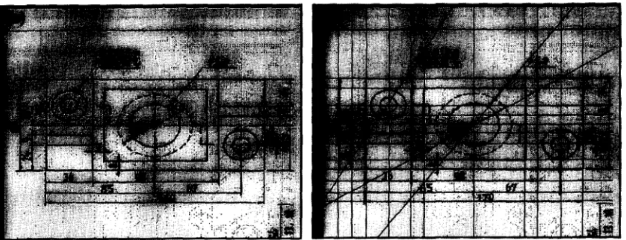
On the other hand, the proposed method can also be used to detect bands, we just need to modify the method by adding a width parameter, which corre- sponds to the shifting distance w, for each band. Fig. 5(a) is the thresholded image of Fig. 3(a). For each
Table 1
The numbers of transforms and the running time needed by HT, RHT, and the proposed method
Fig. 3(b) Fig. 4(b)
q = 180, n = 9 . l , b = 0 . 8 q = 1 8 0 , n = 3 6 . 3 , b = 3 . 8
HT 842220 (7.0 sec.) 3346380 (21.2 sec.)
Random HT 15000 (1.6 sec.) 45000 (5.1 sec.) Proposed method 3923 (1.1 sec.) 71658 (4.5 sec.)
C.-T. Ho, L.-H. Chen /Pattern Recognition Letters 17 (1996) 467-473 473
Fig. 5. The experimental result of applying the proposed band detector. (a) The thresholded image of Fig. 3(a). (b) The detection result of applying the proposed method to (a); two bands are detected.
e d g e p o i n t in the t h r e s h o l d e d i m a g e , a set o f b u d d y p o i n t s is located, a set o f possible p a r a m e t e r s is c o m p u t e d and the c o r r e s p o n d i n g entity is c o u n t e d in a 3-d a c c u m u l a t i o n array. F i n a l l y , a p e a k - f i n d i n g o p e r a t i o n is a p p l i e d to the array, the result is s h o w n in Fig. 5(b).
Acknowledgements
W e w o u l d like to a c k n o w l e d g e the g e n e r o u s sup- port b y the N a t i o n a l S c i e n c e C o u n c i l o f R . O . C . u n d e r c o n t r a c t N S C - 8 3 - 0 4 0 8 - E - 0 0 9 - 0 3 7 .
References
Atiquzzaman, M. (1992). Multiresolution Hough transform - an efficient method of detecting patterns in images. IEEE Trans. Pattern Anal. Mach. lntell. 14, 1090-1095.
Davies, E.R. (1987). A new parameterisation of the straight line and its application for the optimal detection with straight edge.
Pattern Recognition Lett. 6, 1-7.
Duda, R.O. and P.E. Hart (1972). Use of Hough transformation to detect lines and curve in pictures. Comm. ACM 15, 11-15. Hough, P.V.C. (1962). Method and means for recognizing com-
plex pattern. U.S. Patent No. 3069654.
lllingworth, J., and J. Kittler (1987). The adaptive Hough trans- form. IEEE Trans. Pattern Anal. Mach. Intell. 10, 690-698. Leavers, V.F. (1993). Survey: which Hough transform?. CVGIP:
Image Understanding 58, 250-264.
Li, H., M.A. Lavin and R.J. LeMaster (1986). Fast Hough trans- form: a hierarchical approach. CVGIP 36, 640-642. O'Gorman, F., and M.B. Clowes (1976). Finding picture edges
through collinearity of feature points. IEEE Trans. Comput.
25, 449-456.
Xu, L., E. Oja and P. Kultanen (1990). A new curve detection: random Hough transform. Pattern Recognition Lett. 11, 331-338.