Fair Scheduling in Mobile Ad Hoc Networks With
Channel Errors
Hsi-Lu Chao, Student Member, IEEE, and Wanjiun Liao, Member, IEEE
Abstract—We study fair scheduling in ad hoc networks,
ac-counting for channel errors. Since wireless channels are susceptible to failures, to ensure fairness, it may be necessary to compen-sate those flows on error-prone channels. Existing compensation mechanisms need the support of base stations and only work for one-hop wireless channels. Therefore, they are not suitable for multihop wireless networks. Existing fair scheduling protocols for ad hoc networks can be classified into timestamp-based and credit-based approaches. None of them takes channel errors into account. We investigate the compensation issue of fair scheduling and propose a mechanism called Timestamp-Based Compensation Protocol (TBCP) for mobile ad hoc networks. We evaluate the performance of TBCP by simulation and analyze its long-term throughput. The results show that our analytical result provides accurate performance estimation for TBCP.
Index Terms—Channel compensation, fair scheduling, fairness,
wireless ad hoc networks.
I. INTRODUCTION
A
N ad hoc network is a self-organizing wireless network comprised only of mobile nodes. In such a network, nodes are connected via multihop paths and without the support of any preexisting wired infrastructure. In wireless networks, radio spectrum (i.e., bandwidth) is a precious and limited resource. Such a resource should be shared by nodes in a fair way, espe-cially when there is competition for this resource due to unsat-isfied demands.Existing fair scheduling mechanisms in ad hoc networks can be classified into two categories: timestamp based [1], [2] and credit based [3], according to different decision metrics. The timestamp-based mechanisms in [1] and [2] work similarly. In [2], a flow graph must first be generated. Each vertex in the flow graph represents a flow. When two flows contend for the same resource, an edge is added between them. The scheduling discipline in [2] is based on start-time fair queueing (SFQ) [4],
Manuscript received October 15, 2003; revised January 4, 2004; accepted February 21, 2004. The editor coordinating the review of this paper and ap-proving it for publication is Y.-B. Lin. This work was supported in part by the MOE program for Promoting Academic Excellence of Universities under Grant NSC93-2752-E-002-006-PAE and by the National Science Council, Taiwan, under Grant NSC93-2213-E-002-001.
H. L. Chao was with the Department of Electrical Engineering, National Taiwan University, Taipei 106, Taiwan, R.O.C. She is now with the Depart-ment of Computer and Information Science, National Chiao Tung University, Hsinchu, Taiwan, R.O.C.
W. Liao is with the Department of Electrical Engineering, National Taiwan University, Taipei 106, Taiwan, R.O.C.
Digital Object Identifier 10.1109/TWC.2004.842942
and each newly arriving packet is locally assigned a start and a finish tag according to (1).
,
(1)
where is the start tag and is the finish tag of the th packet
of flow ; , , , and are the th packet of
flow , the length of , the arrival time of , and the virtual arrival time of , respectively; is the flow weight of flow , indicating the fraction of link capacity to be shared by . Either tag can be chosen as the service tag. The packet with the smallest service tag is transmitted first. Spatial channel reuse is implemented by means of backoff parameters. Each packet of a flow is associated with a backoff value equal to the number of flows contending for the channel but with smaller service tags. The backoff value is decremented by one at each time slot. Once this value reaches zero, the packet is transmitted.
In [3], a two-tier and cluster-based mechanism is proposed. The network is logically partitioned into clusters, each with a scheduler. Each flow is associated with three parameters: credit,
usage, and excess, where Excess Usage Credit. The
sched-uler assigns time slots to mobiles in the respective cluster based on the first tier algorithm. The mobiles scheduled to send at the next time slot then in turn assign the time slot to the flows de-termined by the second tier algorithm. Each cluster scheduler operates independently. The scheduling disciplines in both al-gorithms are all based on the credit value, i.e., the one with the smallest excess value has the priority to transmit. The unused credit can be accumulated for future use.
The problem in [1]–[3] is that the transmission channels are all assumed error free. This assumption is, however, unrealistic for wireless networks [5] due to their high channel error rates, such as location-dependent errors or bursty errors. In what fol-lows, we first survey the related work on error compensation for wireless networks and then describe our main contribution to the addressed problem for ad hoc networks.
A. Related Work on Error Compensation in Wireless Networks
Existing works proposed to achieve fairness for wireless net-works with channel errors are all based on the support of base stations and work only for one-hop wireless channels [6]–[9].
In [6], the channel-condition independent packet fair queueing (CIF-Q) is proposed. Each session is associated with a parameter called lag to indicate whether the session should be compensated. If a session is not leading and the channel is 1536-1276/$20.00 © 2005 IEEE
error free at its scheduled time, its head-of-line packet is trans-mitted; otherwise, the time slot is released to other sessions. The problem with CIF-Q is that the leading sessions are not allowed to terminate unless all their leads have been paid back, regardless of whether such terminations are caused by broken routes. This property makes CIF-Q an inadequate solution for ad hoc networks, because a connection may be broken due to node movements.
In [7], the idealized wireless fair-queueing (IWFQ) and the wireless packet scheduling (WPS) protocols are proposed. When a session experiences channel errors at its scheduled time, the base station first attempts to swap the slots assigned to this session with other sessions within the same frame. If such an attempt fails, the base station will compensate the error slots of this session in a later frame. Again, this mechanism is not suitable for ad hoc networks due to the need of support from base stations.
In [8], a virtual compensation session is introduced in the scheduling process. The virtual session is a session which al-ways experiences an error-free channel at its scheduled time but does not really generate packets. The slots received by this vir-tual session will be used for compensation, i.e., they will be re-assigned to lagging or handoff sessions. This mechanism, how-ever, does not consider multihop flows. Thus, it is not suitable for ad hoc networks.
In [9], bandwidth-guaranteed fair scheduling with effective excess bandwidth allocation (BGFS-EBA) is proposed. In BGFS-EBA, each flow can be a lagging, leading, or in-synch flow as compared to its bandwidth allocation in an error-free environment. Each flow is associated with a parameter called deadline. The bandwidth resource is first scheduled according to such deadlines and then further allocated based on flow status (i.e., lagging, leading, or in-synch) as in CIF-Q. Unlike other mechanisms, which allow a flow to transmit only in a good state, a flow in BGFS-EBA is allowed to transmit, albeit at lower rates, when its channel is error prone. Again, this mechanism needs the support of base stations. Thus, it is not suitable for ad hoc networks.
B. Problem Specification
It is a challenge to provide channel compensation while sharing resource fairly for ad hoc networks. The challenge is mainly caused by the fully distributed nature of mutlihop wireless networks. In ad hoc networks, there is no support from base stations, and multihop flows passing through different hops are processed in an uncoordinated way. Existing channel compensation mechanisms for wireless networks, however, are mainly designed for single-hop networks with the support of base stations. This renders them inadequate for ad hoc networks.
In this paper, we study fair scheduling, accounting for channel errors for ad hoc networks. In particular, we focus on timestamp-based mechanisms. Existing timestamp-based mechanisms for ad hoc networks (i.e., [1] and [2]) only work for single-hop flows. Implementing fully distributed sched-uling based on timestamps for multihop flows is much more of a challenge. In this paper, we propose a new mechanism called timestamp-based compensation protocol (TBCP), which
is a multihop timestamp-based fair scheduling mechanism providing error compensation for flows experiencing channel errors. We consider a mix of best effort and quality-of-service (QoS) flows in the network, where QoS flows are flows whose minimum bandwidth requirements should be guaranteed. Our objective is to guarantee the minimum bandwidth requirements of QoS flows, while ensuring global fairness for best effort flows. Note that for credit-based mechanisms (e.g., CSAP [3]), unused credits can be accumulated for future use and error compensation is naturally available. As a result, they can be easily extended to handle channel errors.
The rest of this paper is organized as follows. TBCP is de-scribed in Section II. The performance of TBCP is evaluated in Sections III and IV. Finally, the paper is concluded in Section V.
II. TBCP
In TBCP, the scheduling discipline is based on SFQ [4]. The start tag in (1) is selected as the service tag for TBCP. When there is no packet to be sent, the service tag is set to .
A. System Model
The general system model of TBCP is described as follows. 1) A multihop wireless network is considered in which
a TDMA-based system is assumed to operate over a single channel shared by all hosts. The bandwidth is represented as frames of time slots and the slot allo-cation to packets waiting to be transmitted is based on their service tags. Each TDMA frame contains a fixed number of time slots. The network is synchronized on a frame and slot basis, using existing synchronization protocols [10], [11]. Take the tiered adaptive timing synchronization procedure (TATSP) [10] for example. In TATSP, a small set of fast nodes is quickly identi-fied. These nodes are given more chances to send out beacons. Each node should adopt the timing received from any beacon with a timestamp later than its time-stamp.
2) We support two types of flows: best-effort and QoS flows. For QoS flows, the minimum bandwidth requirement is guaranteed and is represented as a frac-tion of one time slot, denoted as in this paper. Thus, for a QoS flow, the value is a positive real number between zero and one; for a best effort flow, the value is always zero.
3) A valid route should be constructed before data packets are transmitted, using whatever ad hoc routing mecha-nisms. For best effort flows, an ad hoc routing protocol (such as [12] and [13]) is used; for QoS flows, QoS routing (such as [14] and [15]) is used. The routing mechanism should also reroute packets on the broken path caused by node movements. The rerouting may be either locally constructed or fully reconstructed from the source to all nodes.
4) Simple admission control is performed at each node during path construction. A flow is admitted only when the sum of the reservation levels (i.e., ) of all
flows, including the newly arriving one is less than or equal to the target link utilization.
5) We consider only short-term channel errors. To avoid resumed flows hogging the channel resource after long-term error conditions, the flows without message exchanges longer than a threshold due to channel errors will be removed from the scheduling. As such, the resumed flows need to compete for the resource as newly arriving flows.
6) The channel state is detected as follows. Each node pe-riodically measures the signal-to-noise ratio (SNR) of the channel. If the SNR value falls below a predefined threshold, the channel is deemed error-prone and the node stops from transmitting packets temporarily. If the SNR value exceeds the predefined threshold again, the transmission resumes.
Note that to better distinguish between the mechanisms with and without implementing compensation, those considering channel errors in their scheduling are referred to as compensa-tion models and those assuming that channels are always error free in their scheduling as error-free models. In addition, the nodes experiencing error states are called channel-error nodes, and those without errors are error-free nodes. Similarly, packets transmitted on error-prone channels are called channel-error packets and those on error-free channels are error-free packets.
B. Multihop Flows
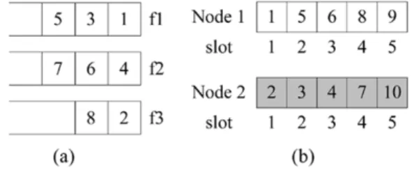
Each node in mobile ad hoc networks acts as both a router and a host. In TBCP, a multihop flow is modeled as mul-tiple single-hop flow segments, and each node schedules the single-hop flows passing through it independently. In TBCP, each end-to-end flow is referred to as a “flow,” and the single-hop flows belonging to a multihop flow are called “flow segments.” For example, flow in Fig. 1 is comprised of five
single-hop flow segments, i.e., , , , , and .
The source and the destination of flow are nodes 1 and 6, respectively. Note that each single-hop flow has one and only one flow segment.
Each flow segment of a multihop flow may be scheduled by different nodes. As a result, even though a downstream flow seg-ment has been assigned a slot, it may not have packets queued to be transmitted unless the upstream flow segments have all been allocated a slot. To solve this problem, a new parameter called
Q-size is defined to correlate multiple flow segments belonging
to the same multihop flow. Each flow is associated with a Q-size parameter at each node on the flow path. This parameter is ini-tialized to zero at all nodes except for the sender, which has a nonzero Q-size depending on the number of packets to be trans-mitted. The Q-size of a flow segment indicates the number of packets received from its previous hop and waiting to be sent to the next hop. A node with nonzero Q-size means at least one of its flow segments has packets waiting to be sent, and this node will choose the least service tag of queued packets as its service tag. Among all nodes with nonzero Q-size values, the node with the least service tag is scheduled for the next time slot.
Fig. 1. Q-size.
C. Normalized Flow Weight
Assume that there are flows passing through node . Let denote the bandwidth share of flow at node (called the flow weight of flow at node in this paper), expressed as
(2) where is the minimum bandwidth requirement of flow , represented as a fraction of the channel bandwidth. Bandwidth share indicates the fraction of channel bandwidth used by flow at node to fairly share the residual bandwidth of node and meet the minimum bandwidth requirement of flow . For example, assume that there are three flows, say, , , and passing through node . Flows and are guaranteed flows, each with a value of 0.2; flow is a best effort flow. Based on (2), the bandwidth share of the three flows at node are
.
In TBCP, the actual bandwidth shared by each flow at node is collaboratively determined by all flows at all nodes in the in-terference range (i.e., nodes located within two hops) of node , not just solely depending on those flows passing through node . Due to a lack of coordination for transmissions, nodes located in the interference range may contend for the channel, and such contention should be considered in the calculation of bandwidth share for each flow. To reflect this fact, the normal-ized flow weight of each flow at node is defined.
Let and denote the two sets of flow segments passing through node and , respectively, where is within two hops of node . Let be the set of nodes, including and all other nodes in its interference range (i.e., two hops). The normalized flow weight of flow segment at node is
(3)
This normalized flow weight is then used to calculate the service tag of flow at node . The number of slots per frame obtained by flow at node is equal to times the number of slots per frame. Note that since the calculations of (2) and (3) are performed independently at each node, different single-hop flow segments of a multihop flow may have different bandwidth shares and different normalized flow weights.
For example, consider two nodes, say and , in an ad hoc network. These two nodes are within the
transmis-sion range of each other. Let indicate the value
Fig. 2. TBCP.
, and that of
is . Thus, the
band-width shares calculated by and are (0.4, 0.4, 0.2) and (0.6, 0.2, 0.2), respectively, and the normalized flow weights of all flows are
.
So far, we have not mentioned how the signaling protocol works for message exchanges among nodes in the interference range. Recall that each TDMA frame is comprised of a fixed number of time slots. The network is synchronized on a frame and slot basis. A frame is comprised of a control phase and a data phase. The signaling messages are exchanged in the control phase. The messages to be exchanged are flooded to a region within two hops (with ) during the control phase. Based on the received messages, the normalized flow weight of each flow at a node can be calculated.
D. TBCP Operations
1) Determination of Packet Transmission Order at a Node: The transmission order of a packet at a node is affected
by three factors: the number of slots per frame the flow can use, the flow’s Q-size at that node, and the service tag of the packet. The normalized flow weight of flow at node is first calculated. Based on , flow at node is allocated
slots per frame, where is the number of slots per frame. The allocated slots may exceed the requirement if the number of packets waiting to be transmitted, i.e., the Q-size of flow , is less than . In this case, the unused slots are released to other flows, and flow will not be compensated with these give-away slots. The transmission order is then determined by the service tag. For example, the numbers in Fig. 2(a) show the packets’ service tags of three flows , , and at node . Assume that each frame is comprised of five slots, and indicates the th packet of flow . The number of slots per frame each flow can use is (2, 2, 1). For flow , the first two least service-tag packets are transmitted, i.e., and . After the comparison with other two flows, the transmission order of
packets at node in Fig. 2(a) is . However,
if has only one packet waiting to be sent, its unused slot will be released to other flows. In this case, the transmission order
arranged by node becomes .
2) Message Exchange: Each node exchanges the
infor-mation about the transmission order of packets determined at step 1) with its neighbors on a per-frame basis. Thus, each node knows the service tags of other nodes and also learns when it can transmit packets. For example, assume that there
are two nodes in an ad hoc network, and the transmission order based on the service tag is shown in Fig. 2(b). Let indicate the th slot of node . The transmission sequence is
, . Note that if
multiple nodes have packets with the same service tag, the tie will be broken based on their node IDs.
Note that the messages are exchanged by flooding with . As such, the exchanged messages are restricted to those neighbors within two hops. The communication overhead of TBCP is mainly caused by such message exchanges within two hops
3) Channel Error Handling: Each node keeps monitoring
its channel state. When the channel is error prone, the node stops exchanging transmission messages with its neighbors. Once the channel recovers, the error-prone node resumes the exchanges. Consequently, if this node has packets with service tags smaller than its neighbors after recovery, these packets still have higher priority to be transmitted. For example, as shown in Fig. 2(b), node 2 experiences an error-prone state at slot 4 during the transmission of frame 1, but the channel recovers before the frame 2 is sent. The modified sequence then becomes
, . Note that one
slot is wasted in this example because messages are exchanged on a per-frame basis.
III. SIMULATIONRESULTS
In this section, TBCP is evaluated via simulation. We com-pare TBCP with TBP, the error-free model of TBCP (i.e., as-suming that channels are error free). We also show CBCP and CSAP [3] (denoted as CBP in this paper) in the figures for com-parison, where CBP and CBCP are the credit-based mechanisms for channel error-free and compensation models, respectively. CBCP differs from CBP in that when a node detects an error state at its scheduled time, the node will inform its scheduler to stop assigning further slots to it. The credit value of this node at the scheduler continues to be accumulated. Thus, once the channel has recovered, the node has a small excess value as com-pared to other error-free nodes, which allows this node to have priority to obtain slots. This node then, in turn, assigns this slot to the flow with the least excess value among all nonzero Q-size flows.
A. Simulation Environment and Performance Metrics
In the simulation, 20 nodes are randomly distributed in a 1000 by 1000-m area. The transmission range of each node is 250 m. Some nodes are randomly selected as flow sources and some as flow destinations. Each flow may either be a best effort or a guaranteed flow and is continuously backlogged. Each packet is assumed to occupy one time slot and has fixed packet length.
We implement spatial channel reuse for both TBP and TBCP in the simulation, using a mechanism similar to that in [2]. Each flow maintains a parameter called backoff, which decides whether it can use the next slot. The backoff value of a flow, say flow , is the number of flows located in flow ’s interference range and with smaller service tags. This backoff value counts down at each time slot. When the backoff value becomes zero, the flow can use the next slot.
The proposed mechanism is evaluated with two scenarios: multihop flows without node mobility and multihop flows with mobility support. The mobility pattern of each node follows the modified random waypoint model [16]. Each node randomly selects a target position and speed to move. The speed selected by a mobile node is within (Min, Max) meters per second. After arriving at the target position, the mobile node stays there for a predefined period of time, called the pause time. The mobile host then randomly selects a new target position and a speed and moves again.
The performance metrics measured in the simulation include the relative network throughput, satisfaction index, and fairness index.
1) Network throughput : this parameter is defined as the summation of all flows’ throughputs achieved by an approach.
2) Relative network throughput : this parameter
is defined as throughput throughput for
the credit-based mechanism and throughput throughput for the timestamp-based mechanism. 3) Satisfaction index : this parameter indicates how
well all QoS flows are satisfied with each approach, considering channel conditions. is defined in a way similar to the definition of the fairness index in [17]. Thus, we only count QoS flows and define it as
, where is the residual band-width share (i.e., flow’s slot usage divided by simula-tion time, less the value) and is set to one if the corresponding is equal to or larger than zero; other-wise, is one minus the shortage divided by its value, and is the number of guaranteed flows. 4) The fairness index : this parameter indicates
how fair the residual bandwidth shared by all flows for each approach is and is defined as in [17], i.e., where is the residual bandwidth share if is equal to or larger than zero; otherwise, is zero, and is the number of flows in an ad hoc network. Note that we do not use the proportional fairness defined in [6]–[8], i.e., , as the fairness index. The reason is for a multihop flow, the single-hop flow segments may not have identical flow weights.
B. Simulation Results
We adopt a two-state discrete Markov chain as in [18] to model wireless channel errors. Let denote the probability that the next time slot is in the good state given that the cur-rent time slot is bad, and let denote the probability that the next time slot is bad given that the current slot is in the good state. The steady-state probabilities and in the good and
error states, respectively, are given by and
.
We first generate ten multihop flows: six guaranteed flows and four best effort flows. and in the error model are set to 0.08 and 0.02, respectively. Thus, the steady-state probabilities and in the good and bad states are 0.8 and 0.2, respectively.
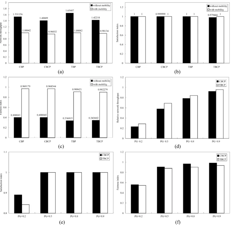
Fig. 3(a) (see black bars) shows the network throughput. We find both CBCP and TBCP have similar network throughput.
This is because the throughput of each multihop flow is deter-mined by the area with the largest congestion degree1it passes
through (here, we call the area the “bottleneck cluster2” for
credit-based schemes and “bottleneck interference range3” for
the timestamp-based schemes) and not solely determined by each cluster (or interference range). Another interesting finding is that TBP has higher network throughput than CBP. This is because the proposed timestamp-based scheme only allows nonzero Q-size nodes to exchange transmission order messages, and thus it is more flexible in slot allocation. Fig. 3(b) and (c) (see black bars) shows their satisfaction and fairness indexes, respectively. We see that both mechanisms still satisfy the de-mands of most QoS flows in this scenario but have low fairness indexes. This is because each multihop flow’s throughput is constrained by the bottleneck cluster. Flows passing through the less congested area will have larger bandwidths, and vice versa. Fortunately, this problem can further be improved when node mobility is supported, as shown in the next scenario.
Next, we make the five multihop flows with mobility. The Min and Max speeds are set to be 10 and 30 m/s, respectively. The network throughput of each approach is shown in Fig. 3(a), and the satisfaction and fairness indexes of each approach are shown in Fig. 3(b) and (c), respectively (see white bars). We find that mobility causes broken routes more frequently, thus degrading network throughput. However, node mobility may in-crease the probability for a flow to change the area in which it is located (i.e., cluster for the credit-based schemes and interfer-ence range for time-stamp based mechanisms). This helps im-prove global fairness.
Finally, we study the impact of channel errors on the pro-posed approaches. We vary the value of but fix all other pa-rameters. The relative network throughput of each approach is shown in Fig. 3(d). As the value of increases, the relative network throughput increases. The reason is that a larger value means more good slots, leading to more successful trans-missions and higher network throughput. The satisfaction and fairness indexes of each setting are shown in Fig. 3(e) and (f), respectively. Since a larger value makes more good slots, the probability to satisfy QoS flows is higher. Thus, it gives a higher satisfaction index. A larger value also increases the opportunity for a node to be compensated after its channel re-covers and thus has a higher fairness index.
IV. PERFORMANCEANALYSIS
In this section, we analyze the long-term throughputs of CBCP and TBCP. In this analysis, we do not consider node mobility and ignore spatial channel reuse. Each mechanism is analyzed with the two-state channel errors.
A. CBCP
We calculate the throughput of CBCP. Suppose that the net-work is partitioned into clusters. Without loss of generality,
1The congestion degree of a cluster is defined as the total reservation level
recorded by the scheduler.
2The bottleneck cluster of a network is the cluster that is the most congested,
i.e., with the highest Resv value.
3The bottleneck interference range of a network is the two-hop area with the
Fig. 3. Simulation results: (a) Network throughput, (b) satisfaction index, (c) fairness index, (d) relative network throughput, (e) satisfaction index for different P values, and (f) fairness index for different P values.
the clusters are sorted in a descending order of the
conges-tion degree, i.e., .
Let denote the number of flow segments in cluster and denote the number of flow segments in both clusters and . Let denote the set of flows in cluster and de-note the set of flows in both clusters and . Assume that the scheduler of cluster manages flow segments. The residual bandwidth shared by flow in cluster is calculated as
, and the total bandwidth used by
flow in cluster is given by . The throughput
of flow is defined as , where is the number of
packets received at the destination node, and is the measure-ment window size.
1) Estimated Throughput: We consider the two-state error
model. The average number of error-free slots obtained by each node is , where is the steady-state probability of the good state. For the most congested cluster, i.e., cluster 1, each flow segment’s throughput is proportional to its , as follows:
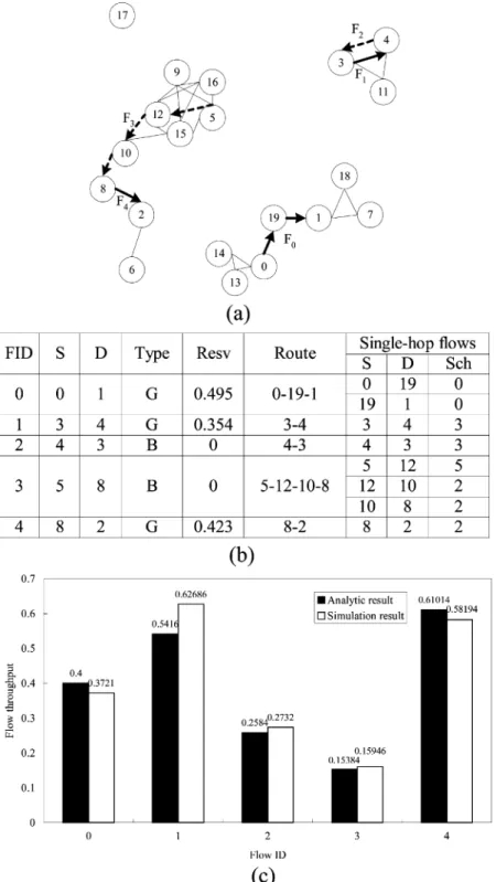
Fig. 4. Analytical result versus simulation result for CBCP: (a) network topology, (b) flow information, and (c) result comparisons. Similarly, the throughputs of those flows in cluster 2 but not
in cluster 1 can be calculated as
(5) Assume the bottleneck of flow segment is in cluster . Let denote the set of flows in cluster but their bottlenecks are
in more congested clusters than cluster (i.e., clusters , or ) and be the set of flows in less congested clusters
(i.e., ). For all flows in , indicates the
bandwidth share of flow segment in its bottleneck cluster . Let denote the number of flow segments in set . Therefore, the throughput of flow segment is expressed as
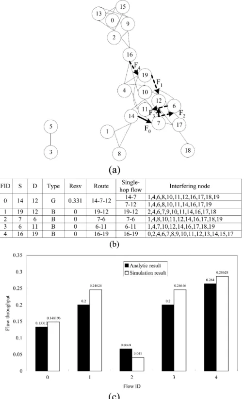
Fig. 5. Analytical result versus simulation results for TBCP: (a) network topology, (b) information of flows and the corresponding interfering nodes, and (c) result comparisons.
For those flows passing through both clusters and , and , their shares of residual bandwidth are constrained by the more congested cluster, i.e., cluster . Thus, they will release some resources to the flows in cluster but not in cluster . Based on this concept, to calculate the throughputs of flows bottlenecked at cluster , we should first recursively derive the flow segments’
throughputs bottlenecked at cluster .
Therefore, for a multihop flow, its estimated flow throughput
is , where is a path node and is the flow path.
2) Analytical Versus Simulation Results: We verify our
analysis via simulation. Five flows are randomly generated in the same network as in Section III: three guaranteed flows and two best effort flows. The network topology and flow information are shown in Fig. 4(a) and (b). The comparison of the analytical result with the simulation result is shown in Fig. 4(c). We see that our analytical model provides very good estimation for the performance of CBCP.
B. TBCP
In an ad hoc network, a transmitting node, say node , will interfere with another node, say , if either condition holds.
1) Node is within the transmission range of node and is the receiver of another flow segment.
2) Node is within the transmission range of node ’s corresponding receiver and is the sender of another flow segment.
Unlike CBCP, TBCP has no schedulers to implement coordi-nation. When a node is transmitting, those nodes within its two hops are interfered with. Therefore, the following analysis deals with this issue by calculating a flow’s normalized weight.
1) Estimated Throughput: We consider the two-state error
model. Assume there are nodes in the ad hoc network. The average number of error-free slots for a node is , where is the measurement window, and is the steady-state prob-ability of the good state. Let indicate the set of flow seg-ments passing through node , and represents the set of flow segments within node ’s interference range. For each flow segment passing through node , its bandwidth share is , where is the number of flow segments managed by node . The normalized flow
weight of is calculated as . The
corresponding flow throughput of flow is given by
(7) For a multihop flow, its estimated flow throughput is
, where is a path node and is the flow path.
2) Analytical Versus Simulation Results: We randomly
gen-erate five flows in the simulation: four best effort flows and one guaranteed flow. The node graph is in Fig. 5(a). Furthermore, the information of flows and the corresponding interfering nodes is shown in Fig. 5(b). The comparison with simulation results is shown in Fig. 5(c). Again, we see that our analytical model pro-vides accurate estimation for the performance of TBCP.
V. CONCLUSION
In this paper, we discuss the channel compensation issue of fair scheduling and propose one such mechanism called TBCP for mobile multihop networks. TBCP supports multihop flows and performs well when node mobility is supported. We de-scribe the detailed operation of TBCP and conduct simulations to evaluate its performance. From the simulation results, we demonstrate that TBCP satisfies QoS flow demands and pro-vides global fairness for best effort flows. We also show that mobility helps break the locality problem for multihop flows. Finally, we analyze the flow throughputs of CBCP and TBCP and verify the analytical result with simulation. The results show that our analytical results provide accurate performance estima-tions for the proposed mechanisms.
This paper addresses fair scheduling for multimedia mobile ad hoc networks with channel errors. The QoS demands of flows
basically are described via bandwidth. In the future, we will investigate fair scheduling with other QoS metrics such as delay or delay jitter for ad hoc networks.
REFERENCES
[1] H. Luo and S. Lu, “A topology-independent fair queueing model in ad
hoc wireless networks,” in Proc. IEEE Int. Conf. Network Protocol, Nov.
2000.
[2] , “A self-coordinating approach to distributed fair queueing in ad
hoc wireless networks,” in Proc. IEEE INFOCOM, Apr. 2001.
[3] H. L. Chao and W. Liao, “Fair scheduling with QoS support in ad hoc networks,” in Proc. IEEE Conf. Local Computer Networks, Nov. 2002. [4] P. Goyal, H. M. Vin, and H. Cheng, “Start-time fair queueing: A sched-uling algorithm for integrated services packet switching networks,”
IEEE/ACM Trans. Networking, vol. 5, no. 5, Oct. 1997.
[5] Y. Cao and V. O. K. Li, “Scheduling algorithms for broadband wireless networks,” Proc. IEEE, vol. 89, no. 1, pp. 76–87, Jan. 2001.
[6] T. S. E. Ng, I. Stoica, and H. Zhang, “Packet fair queueing algorithm for wireless networks with location-dependent errors,” in Proc. IEEE
INFOCOM, 1998.
[7] S. Lu, V. Bharghavan, and R. Srikant, “Fair scheduling in wireless packet networks,” IEEE/ACM Trans. Networking, vol. 7, no. 4, Aug. 1999. [8] S. Lee, K. Kim, and A. Ahmad, “Channel error and handoff
compensa-tion scheme for fair queueing algorithms in wireless networks,” in Proc.
IEEE Int. Comput. Conf., 2002.
[9] Y. Cao and V. O. K. Li, “Wireless packet scheduling for two-state link models,” in Proc. IEEE Globecom, 2002.
[10] L. Huang and T.-H. Lai, “On the scalability of IEEE 802.11 ad hoc net-works,” in Proc. MobiHoc, 2002.
[11] T.-H. Lai and D. Zhou, “Efficient and scalable IEEE 802.11 ad-hoc-mode timing synchronization function,” in Proc. 17th IEEE Int. Conf.
Advanced Information Networking Applicat., 2003.
[12] C. E. Perkins and E. M. Royer, “Ad-hoc on demand distance vector routing,” in Proc. 2nd IEEE Workshop Mobile Computing Systems
Ap-plicat., Feb. 1999, pp. 90–100.
[13] C. E. Perkins and P. Bhagwat, “Highly dynamic destination-sequenced distance-vector routing (DSDV) for mobile computers,” in Proc. ACM
SIGCOMM ’94, pp. 234–244.
[14] S. Chen and K. Nahrstedt, “Distributed quality-of-service routing in
ad hoc networks,” IEEE J. Select. Areas Commun., vol. 17, no. 8, pp.
1488–1505, Aug. 1999.
[15] C. R. Lin and J.-S. Liu, “QoS routing in ad hoc wireless networks,” IEEE
J. Select. Areas Commun., vol. 17, no. 8, pp. 1426–1438, Aug. 1999.
[16] J. Yoon, M. Liu, and B. Noble, “Random waypoint considered harmful,” in Proc. IEEE INFOCOM, Apr. 2003.
[17] R. K. Jain, D. W. Chiu, and W. R. Hawe, “A quantitative measure of fairness and discrimination for resource allocation in shared computer system,”, DEC Tech. Rep. DEC-TR-301, 1984.
[18] E. O. Elliot, “Estimates of error rates for codes on burst-noise channels,”
Bell Syst. Tech. J., vol. 42, Sep. 1963.
Hsi-Lu Chao (S’03) was born in Taiwan, R.O.C.,
in 1970. She received the B.S. degree in electronic engineering from Fengchia University, Taiwan, in 1992, the M.S. degree in electrical engineering from the University of Southern California, Los Angeles, in 1996, and the Ph.D. degree in electrical engineering from the National Taiwan University, Taiwan, in 2004.
Since August 2004, she has been an Assistant Pro-fessor in the Department of Computer and Informa-tion Science, NaInforma-tional Chiao Tung University. Her re-search interests include wireless communication and QoS issues in ad hoc net-works.
Wanjiun Liao (S’96–M’97) received the B.S. and
M.S. degrees from National Chiao Tung University, Taiwan, R.O.C., in 1990 and 1992, respectively, and the Ph.D. degree in electrical engineering from the University of Southern California, Los Angeles, in 1997.
She joined the Department of Electrical Engi-neering, National Taiwan University (NTU), Taipei, Taiwan, as an Assistant Professor in 1997. Since August 2000, she has been an Associate Professor. Her research interests include wireless networks, overlay networks, and broadband Internet.
Dr. Liao is currently an Associate Editor of IEEE TRANSACTIONS ON
WIRELESS COMMUNICATIONS. Two papers she co-authored with her stu-dents received the Best Student Paper Award of the First IEEE International Conferences on Multimedia and Expo (ICME), in 2000, and the Best Paper Award of the First International Conference on Communication, Circuits and Systems (IEEE Communication Press), in 2002. She was elected as one of Ten Distinguished Young Women in Taiwan in 2000 and is listed in the Marquis