Three-Dimensional Noniterative Full-Vectorial
Beam Propagation Method Based on the
Alternating Direction Implicit Method
Yu-li Hsueh, Ming-chuan Yang, and Hung-chun Chang,
Member, IEEE, Member, OSAAbstract— The alternating direction implicit (ADI) method is adopted in the full-vectorial beam propagation formulation, which was discretized in the longitudinal direction via the stan-dard Crank–Nicholson scheme. Through proper operator de-composition, operator inversions for the cross-coupling terms existing in the full-vectorial formulation are avoided and second-order accuracy along the propagation direction is achieved in the proposed algorithm. With the aid of the ADI method, our full-vectorial algorithm also has good performance in efficiency. This implicit scheme can theoretically be shown to be numeri-cally unconditionally stable. Several numerical simulations have been performed and compared with those obtained by the finite difference mode-solving scheme based on the shifted inverse power method (SIPM) in order to examine the accuracy of our algorithm.
Index Terms— Alternating direction implicit (ADI) method, beam propagation method (BPM), full-vectorial field propaga-tion, optical waveguides.
I. INTRODUCTION
T
HE beam propagation method (BPM) is at present the most widely used tool employed in the study of optical devices, largely owing to its numerical speed and simplicity [1]. Basically, it constructs a relation between the electro-magnetic fields in two axially separated parallel planes, i.e., the field distribution in one plane is calculated numerically from the distribution in the preceding plane. This procedure is recursively implemented, thus completing the simulation of wave propagation step by step with an arbitrary excitation.Discretizing the BPM formulas in three dimensions via the standard Crank–Nicholson scheme results in an implicit relation between two axially separated parallel planes, and it requires operator inversions to complete the propagation. Manuscript received October 12, 1998; revised June 29, 1999. This work was supported in part by the National Science Council of the Republic of China under Grants NSC87-2215-E002-008 and NSC88-2215-E002-015.
Y. Hsueh was with the Graduate Institute of Electro-Optical Engineering, National Taiwan University, Taipei, Taiwan 106-17 R.O.C. He is now with the Department of Electrical Engineering, Stanford University, Stanford, CA 94305 USA.
M. Yang was with the Graduate Institute of Electro-Optical Engineering, National Taiwan University, Taipei, Taiwan 106-17 R.O.C. He is now with the Chinese Air Force Headquarters, Taipei, Taiwan 106 Republic of China.
H. Chang is with the Department of Electrical Engineering, the Graduate Institute of Electro-Optical Engineering, and the Graduate Institute of Com-munication Engineering, National Taiwan University, Taipei, Taiwan 106-17 R.O.C.
Publisher Item Identifier S 0733-8724(99)08928-8.
Several different approaches have been used to perform the operator inversion [2]–[4]. A widely adopted approach is to use the relaxation methods, in which an inversion is initially guessed and successively modified via feedback mechanisms [5]. The successive over relaxation method and the conjugate gradient method represent typical algorithms [6]. Because of the iterative nature, it may require a lot of iterations to assure the accuracy. Besides, the iterative process not only is time-consuming but also cannot guarantee convergency in some cases. Therefore, the main disadvantages of the relaxation methods are the efficiency and divergence problems. In this paper we seek another way to perform the operator inversion. The alternating direction implicit (ADI) method is a non-iterative procedure for solving multidimensional partial dif-ferential equations [6]. Yamauch et al. [7] proposed a three-dimensional (3-D) BPM algorithm based on the ADI method, which was a scalar algorithm with the operator inversion implemented via the ADI method. Algorithms based on the semivectorial wave equation were also proposed [8]. How-ever, full-vectorial algorithms have not been well developed until recently due to the difficulties resulting from the cross-coupling terms. To avoid performing the operator inversion of the cross-coupling terms, a full-vectorial algorithm was proposed by Mansour et al. [9], in which the preceding electric field was used to estimate the central-point field. It is not a Crank–Nicholson approach, and hence is only of first-order accuracy in the direction. The explicit form of the cross-coupling terms may also become a problem in stability. On the other hand, the algorithm of [9] was proposed to work together with a smoothing digital filter, which is doubtful in some cases especially when the fields contain high frequency components.
In this paper we propose a 3-D full-vectorial BPM algorithm purely based on the standard Crank–Nicholson scheme and the ADI method. In so doing, our proposed algorithm is of second-order accuracy in the direction, and numerical stability is also assured thanks to the pure implicit form. Because of the noniterative nature of the ADI method, our algorithm also has very good performance in speed. Section II gives the mathematical formulation for the proposed BPM algorithm. Several numerical examples are presented in Section III and the BPM calculation is compared with that employing a finite difference mode-solving scheme based on the shifted inverse power method. The conclusion is drawn in Section IV. 0733–8724/99$10.00 1999 IEEE
II. MATHEMATICAL FORMULATION
We derive the formulations for electric fields here. Formu-lations for magnetic fields can be derived in the same way. Starting from Maxwell’s equations, the vector wave equation for the time-harmonic electric field in a linear, isotropic, and time-invariant medium is derived as
(1)
where is the refractive index as a function of position, and is the wave number in vacuum.
If the refractive index does not vary along the direction, or if the variation is very slow compared with its and dependences, the propagation of the electromagnetic wave is governed by two coupled equations with and components only. By defining an envelope field such that
(the slowly varying envelope approximation), and considering the and components in (1), we obtain
(2) where (3) (4) (5) (6)
From (2)–(6) it is clear that and denote the cross-coupling effects between the two transverse fields.
For simplicity, we rewrite (2) as
(7)
which is a second-order partial differential equation describing the transverse field . If we adopt the paraxial assumption here, the second-order derivative term is dropped off, and (7) becomes the full-vectorial paraxial BPM equation
(8)
which is a first-order partial differential equation to be solved as an initial value problem. We shall discretize (8) via the Crank–Nicholson scheme and evaluate it step by step with the aid of the ADI method.
Equation (8) can be rewritten in an alternative form
(9) where and denote the -dependent and the -dependent parts of , respectively, with
(10) (11)
Similarly, and denote the -dependent and the
-dependent parts of , respectively, with
(12)
(13)
while and denote the
cross-coupling terms.
In the semivectorial formulation the cross-coupling terms are assumed negligible, resulting in
(14) (15) Equations (14) and (15) can be individually evaluated via the standard ADI method [8]. For (14), the discretization form becomes
(16) or
(17) Implementing the ADI method by adding second-order error terms to (17) yields
(18) or
In so doing, it becomes not difficult to perform the operator inversion in each substep, and the inserted error terms do not reduce the accuracy, since the Crank–Nicholson scheme is also of second-order accuracy.
But in the full-vectorial formulation the extra cross-coupling terms become an impediment to implement the ADI method. Discretizing (9) with the Crank–Nicholson scheme we obtain
(20)
(21) If and are neglected, (20) and (21) reduce to the semivectorial formulation discussed above. On the contrary, if and are considered, it is not so trivial to implement the operator inversion with the ADI method, since and can not be inversed via the ADI method. In [9], (20) and (21) are approximated by
(22)
(23)
that is, and are used to replace
and , respectively, in order to avoid
performing the operator inversion of and . Such treatment of the cross-coupling terms is similar to the simple Euler method, and hence is only of first-order accuracy in the direction. Furthermore, because of the explicit form, the stability is doubtful. In fact, the algorithm of (22) and (23) was proposed to work together with a digital low-pass filter in order to filter out extra numerical noises in [9]. Here, we propose an alternative formulation to achieve an algorithm of second-order accuracy.
Rewrite (9) as
(24)
After discretizing with the Crank–Nicholson scheme, we ob-tain
(25)
Adopting the ADI method, (25) becomes
(26) It can be easily proven that and are interchangeable. To accomplish propagation, the electric field is multiplied by , divided by , multiplied by , and finally divided
by , or
(27) The operator multiplication in (27) is trivial, and the operator inversion is also not difficult. For example, if we are going to perform the inversion of
(28) or
(29) We can formally solve the equation
first in order to obtain , and then solve
to obtain .
Since this formulation is a pure Crank–Nicholson scheme together with the ADI method, it is a scheme of second-order accuracy in the direction. It can theoretically be shown by the von Neumann analysis [6] that (27) is numerically unconditionally stable.
In our implementation the reference refractive index is adaptively chosen during propagation. To fulfill the slowly varying envelope approximation, should be chosen such that the variations of transverse fields along the longitudinal direction are minimized, and the optimum refractive index should be the average of the effective indexes of all the propagating modes involved in the propagation process [5]. We use Rayleigh quotient at each step to adaptively choose the optimum reference refractive index. From Rayleigh quotient the reference refractive index can be obtained by
(30)
where is the adjoint of the electric field , and is that in (7).
To implement the transverse derivatives for operator , instead of using the graded-index assumption which is ques-tionable especially in strongly guiding structures, we use the
(a)
(b)
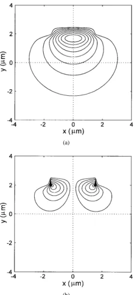
Fig. 1. Contours of the electric field distributions of thex-polarized HE11
mode of a step-index optical fiber. (a)Exand (b)Ey.
finite difference schemes in and directions similar to those in [10] and [11], in which the finite difference schemes can assure truncation errors of second order in the transverse directions.
For boundaries of the numerical window, both the transpar-ent boundary condition (TBC) [12] and the perfectly matched layer (PML) [13], [14] boundary condition can be adopted in our algorithm in order to absorb outgoing waves.
III. NUMERICAL RESULTS ANDCOMPARISONS To verify the practicality and accuracy of the proposed 3-D full-vectorial BPM algorithm, we report four numerical examples.
As a first example, we investigate a step-index single-mode optical fiber, whose exact analytical solutions can be used for an easy comparison. The refractive indexes of the core
and the cladding are taken as and ,
respectively. The radius is m and the wavelength is m. Initially we launch the LP mode and obtain the guided mode profile in the output plane after propagating a long distance of 5 mm. We set the discretizations with
m and m. Fig. 1 shows
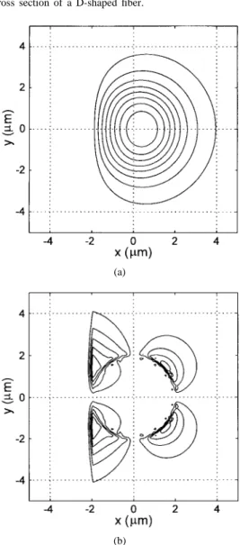
Fig. 2. Cross section of a D-shaped fiber.
(a)
(b)
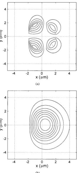
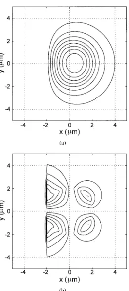
Fig. 3. Contours of the electric field distributions of thex-polarized guided mode of the D-shaped fiber withd = 0. (a) Exand (b)Ey.
the final electric field distribution at mm, which is essentially identical to that of the true HE11 mode. Fig. 1(a)
and (b) depicts the dominant component and the minor component, respectively, of the -polarized mode. The ratio of the maximum magnitudes between and is found to be about 9.95 10 in this case. The calculated effective index
(a)
(b)
Fig. 4. Contours of the electric field distributions of they-polarized guided mode of the D-shaped fiber withd = 0. (a) Ex and (b)Ey.
is . Compared with the exact effective
index , the difference is on the order
of , which is very small. The accuracy can be further improved by using finer discretization grids.
The second example deals with the D-shaped fiber structure, which is a fiber with one side polished, producing the D-shaped cladding. As shown in Fig. 2, the refractive indexes of the core, the cladding, and the vacuum are taken as ,
, and , respectively. As in the first
example, the radius of the core is 2 m and the wavelength
is m. The distance between the core and the
interface is a variable parameter and is denoted as . Initially we launch the LP01 mode of the fiber, propagating a long
distance of 2 mm, and obtaining the guided mode profile in the output plane. We simulate the propagation on the structure with the full-vectorial BPM algorithm for the electric fields and the magnetic fields, respectively. The differences in the calculations involving electric and magnetic fields are basically
in the transverse operators , and in (3)–(6),
and the transverse operators for magnetic fields can be derived from Maxwell’s equations in a similar manner as those for electric fields. The discretizations in the simulation are set
(a)
(b)
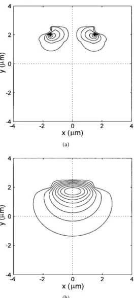
Fig. 5. Contours of the magnetic field distributions of thex-polarized guided mode of the D-shaped fiber withd = 0. (a) Hxand (b)Hy.
with m. Figs. 3 and 4 show the
contours of the final electric field distributions for for the -polarized and the -polarized guided modes, respectively, and Figs. 5 and 6 show the corresponding magnetic field distributions. The ratios of the maximum magnitudes between the minor and the dominant components for Figs. 3–6 are
found to be 1.40 10 , 1.04 10 , 7.20 10 , and
9.05 10 , respectively. The field patterns are found to be identical to those obtained by a finite difference mode-solving scheme based on the shifted inverse power method (SIPM) and with the same transverse discretizations. The SIPM algorithm can provide guided mode solutions with high accuracy. The accuracy of the propagation constant of the guided mode obtained by our SIPM code is found to be up to at least seven effective digits as compared with the theoretical values of certain step-index fiber structures. We analyze three cases with different ’s, and the calculated effective indexes are listed in Tables I and II. It can be seen that the effective indexes obtained by the 3-D BPM agree very well with those obtained by the SIPM, with differences at most on the order of 10 . The proposed BPM algorithm can thus be applied to such mode-solving problems with high accuracy.
(a)
(b)
Fig. 6. Contours of the magnetic field distributions of they-polarized guided mode of the D-shaped fiber withd = 0. (a) Hx and (b)Hy.
TABLE I
COMPARISON OFEFFECTIVEINDEXES FOR THED-SHAPEDFIBERCASE
OBTAINEDUSING THEELECTRIC-FIELDBPMAND THESIPM
TABLE II
COMPARISON OFEFFECTIVEINDEXES FOR THED-SHAPEDFIBERCASE
OBTAINEDUSING THEMAGNETIC-FIELDBPMAND THESIPM
The third example deals with a strongly guiding waveguide structure, which is not easy to be analyzed by conventional vectorial BPM’s. The structure is shown in Fig. 7, which a rib waveguide with refractive indexes of the substrate, the
Fig. 7. Cross section of a rib waveguide.
(a)
(b)
Fig. 8. Contours of the electric field distributions of thex-polarized guided mode of the rib waveguide. (a)Ex and (b)Ey.
guiding layer, and the cover layer being ,
and , respectively. The dimensions are m,
m, and the wavelength is taken to be 1.55 m. We analyze the structure with the BPM algorithm for the electric and magnetic fields and set the discretizations as m. Sometimes simulating with the magnetic fields is preferable because it has the advantage that
(a)
(b)
Fig. 9. Contours of the electric field distributions of they-polarized guided mode of the rib waveguide. (a)Exand (b)Ey.
magnetic fields are always continuous at the interfaces, and thus numerical noises produced by discontinuous electric fields at these interfaces are avoided.
By launching a Gaussian profile in the initial plane and propagating a long distance of 2 mm, the guided mode field distributions are obtained in the final plane. Figs. 8 and 9 show the electric-field contours of the -polarized and the -polarized guided modes, respectively, and Figs. 10 and 11 show the magnetic-field contours of the -polarized and the -polarized guided modes, respectively. The ratios of the maximum magnitudes between the minor and the dominant
components are 4.02 10 4.11 10 2.49 10
and 2.54 10 for Figs. 8–11, respectively, which are significantly larger than the ratios in the previous examples since the present structure is a more strongly guiding one. The effective indexes are calculated and listed in Tables III and IV. Compared with the SIPM results, the differences are only on the order of 10 –10 .
Finally, we consider a polished-type optical fiber coupler [15]. The side view of the polished-type coupler is shown in Fig. 12. Two cores are curved in parabolic shapes, and between them an index-matching liquid layer (a slab layer)
(a)
(b)
Fig. 10. Contours of the magnetic field distributions of the x-polarized guided mode of the rib waveguide. (a)Hx and (b)Hy.
is introduced. The refractive indexes of the core and the
cladding are and , respectively. The
core radius is 2 m, the radius of curvature of the curved
core is cm, the wavelength is m,
and the total longitudinal length considered is 2600 m. The refractive index and the width of the liquid layer are taken to be variable parameters. We simulate the coupler performance by launching the fundamental mode in the initial plane of one core, propagating through the coupler, and obtaining the output power distribution in the final plane. The discretizations
used are m and m. The
output power transfer ratio is desired in our simulation. We obtain with our 3-D algorithm the power transfer ratios for several coupler structures with different liquid layer indexes and widths, and compare the results with those obtained by the SIPM approach as described below.
To get the output coupled power of the coupler as shown in Fig. 10 based on the SIPM mode-solving approach, we first calculate the local coupling coefficient defined as
(a)
(b)
Fig. 11. Contours of the magnetic field distributions of the y-polarized guided mode of the ribwaveguide. (a)Hx and (b)Hy.
Fig. 12. Cross section of the side view of the polished-type optical fiber coupler.
where and are the propagation constants
of the symmetric and antisymmetric modes of the coupler
TABLE III
COMPARISON OFEFFECTIVEINDEXES FOR THERIBWAVEGUIDECASE
OBTAINEDUSING THEELECTRIC-FIELDBPMAND THESIPM
TABLE IV
COMPARISON OFEFFECTIVEINDEXES FOR THERIBWAVEGUIDECASE
OBTAINEDUSING THEMAGNETIC-FIELDBPMAND THESIPM
TABLE V
COMPARISON OFPOWERTRANSFERRATIOS FOR THEPOLISHED-TYPE
COUPLERSOBTAINEDUSING THE3-D BPMAND THESIPM
structure, respectively, at a certain distance from the waist of the coupler . Since the geometrical structure of the coupler is symmetric with respect to the plane, the
coupled power can be calculated as
(32) where is the power injected into the input fiber. In
our calculation is solved every 100 m from to
m, with those values at other points determined by interpolation using the cubic spline method to save the computing time. The power transfer ratios obtained by the BPM and the SIPM approach are listed in Table V. Four coupler structures with different liquid layer refractive indexes and widths are considered. From the table it is seen that the dif-ferences are on the order of a few thousandths, demonstrating again that our proposed BPM algorithm provides simulation results of high accuracy.
IV. CONCLUSION
A 3-D noniterative full-vectorial beam propagation method purely based on the Crank–Nicholson scheme and the ADI method is proposed. The axial component is discretized by the Crank–Nicholson scheme, in which the necessary operator inversions are performed by the ADI method. With proper operator decomposition we have successfully applied the ADI method to the full-vectorial formulation and avoided perform-ing the operator inversion for the cross-couplperform-ing terms. The proposed algorithm is of second-order accuracy along the propagation direction, and it can be theoretically shown that the implicit discretization scheme is numerically uncondition-ally stable. Due to the noniterative nature of ADI method, our algorithm has good performance in efficiency compared with those using the relaxation approaches. The accuracy of our algorithm is examined through several numerical examples
by comparing our results with the exact effective index of an optical fiber and those obtained by the finite difference mode-solving scheme based on the shifted inverse power method.
REFERENCES
[1] D. Yevick, “A guide to electric field propagation techniques for guided-wave optics,” Opt. Quantum Electron., vol. 26, pp. S185–S197, 1994. [2] D. Yevick and B. Hermansson, “Efficient beam propagation techniques,”
IEEE J. Quantum Electron., vol. 26, pp. 109–112, 1990.
[3] A. Kunz, F. Zimulinda, and W. E. Heinlein, “Fast three-dimensional split-step algorithm for vectorial wave propagation in integrated optics,”
IEEE Photon. Technol. Lett., vol. 5, pp. 1073–1076, 1993.
[4] E. E. Kriezis and A. G. Papagiannakis, “A three-dimensional full vectorial beam propagation method forz-dependent structures,” IEEE
J. Quantum Electron., vol. 33, pp. 883–890, 1997.
[5] W. P. Huang and C. L. Xu, “Simulation of three-dimensional opti-cal waveguides by a full-vector beam propagation method,” IEEE J.
Quantum Electron., vol. 29, pp. 2639–2649, 1993.
[6] W. H. Press, S. A. Teukolsky, W. T. Vetterling, and B. P. Flannery,
Numerical Recipes in C—The Art of Scientific Computing, 2nd ed. New York: Cambridge University Press, 1992.
[7] J. Yamauchi, T. Ando, and H. Nakano, “Beam-propagation analysis of optical fibers by alternating direction implicit method,” Electron. Lett., vol. 27, pp. 1663–1665, 1991.
[8] P. L. Liu and B. J. Li, “Semivectorial beam-propagation method for analyzing polarized modes of rib waveguides,” IEEE J. Quantum
Electron., vol. 28, pp. 778–782, 1992.
[9] I. Mansour, A. D. Capobianco, and C. Rosa, “Noniterative vectorial beam propagation method with a smoothing digital filter,” J. Lightwave
Technol., vol. 14, pp. 908–913, 1996.
[10] C. Vassallo, “Improvement of finite difference methods for step-index optical waveguides,” Inst. Elec. Eng. Proc.— J., 1992, vol. 139, pp. 137–142.
[11] J. Yamauchi, M. Sekiguchi, O. Uchiyama, J. Shibayama, and H. Nakano, “Modified finite-difference formula for the analysis of semivectorial modes in step-index optical waveguides,” IEEE Photon. Technol. Lett., vol. 9, pp. 961–963, 1997.
[12] G. R. Hadley, “Transparent boundary condition for the beam propagation method,” IEEE J. Quantum Electron., vol. 28, pp. 363–370, 1992. [13] J. P. Ber´enger, “A perfectly matched layer for the absorption of
electromagnetic waves,” J. Comput. Phys., vol. 114, pp. 185–200, 1994. [14] W. P. Huang, C. L. Xu, W. Lui, and K. Yokoyama, “The perfectly matched layer (PML) boundary condition for the beam propagation method,” IEEE Photon. Technol. Lett., vol. 8, pp. 649–654, 1996. [15] M. Digonnet and H. J. Shaw, “Analysis of a tunable single mode optical
fiber coupler,” IEEE J. Quantum Electron., vol. 18, pp. 746–754, 1982.
Yu-li Hsueh was born in Taipei, Taiwan, R.O.C., on July 28, 1974. He received the B.S. degree in electrical engineering and the M.S. degree in electrooptical engineering from National Taiwan University, Taipei, in 1996 and 1998, respectively.
His research interests include theory and appli-cations of guided wave structures and numerical simulation techniques for integrated optical devices.
Ming-chuan Yang was born in Taipei, Taiwan, R.O.C., on September 1, 1974. He received the B.S. degree in electrical engineering and the M.S. degree in electro-optical engineering from the National Taiwan University in 1996 and 1998, respectively.
His research interests include the application of fiber-optic devices and the waveguide structures for optoelectronics.
Hung-chun Chang (S’78–M’83) was born in Taipei, Taiwan, R.O.C., on February 8, 1954. He received the B.S. degree from National Taiwan University, Taipei, R.O.C., in 1976 and the M.S. and Ph.D. degrees from Stanford University, Stanford, CA, in 1980 and 1983, respectively, all in electrical engineering.
From 1978 to 1984, he was with the Space, Telecommunications, and Radioscience Laboratory of Stanford University. In August 1984, he joined the faculty of the Electrical Engineering Department of National Taiwan University, where he is currently a Professor. He served as Vice-chairman of the EE Department from 1989 to 1991, and Chairman of the newly-established Graduate Institute of Electro-Optical Engineering at the same University from 1992 to 1998. His current research interests include the theory, design, and application of guided-wave structures and devices for fiber optics, integrated optics, optoelectronics, and microwave and millimeter-wave circuits.
Dr. Chang is a member of Sigma Xi, the Phi Tau Phi Scholastic Honor Society, the Chinese Institute of Engineers, the Photonics Society of Chinese-Americans, the Optical Society of America (OSA), and China/SRS (Taipei) National Committee (a Standing Committee member during 1988–1993) and Commission H of U.S. National Committee of the International Union of Radio Science (URSI). In 1987, he was among the recipients of the Young Scientists Award at the URSI XXIInd General Assembly. In 1993, he was one of the recipients of the Distinguished Teaching Award sponsored by the Ministry of Education of the Republic of China.