Analysis of scheduling parallel tasks on
hypercube systems
J.-F. L i n and S.-J. C h e n
Indexinr rerms: Muhiprocessing sq’srenzs, Pordlel prwe.wirig. Scheduling
The problem of scheduling independent parallel talks with the consideration of setup time on a d-dimensional hypercube system is investigated. The objective of this problem is to find a schedule with minimum finish time; such a scheduling problem is NP-hard. Therefore. a heuristic algorithm is proposed and its performance hound derived.
Introduction: The problems of scheduling tasks on multiprocessor systems have been extensively studied for a long time. Conven- tional approaches were proposed for the problem of scheduling each task on only one processor at a time, which is referred to as the conventional task scheduling problem. Finding a minimum finish time nonpre-emptive schedule for this type of problem on an m-processor system, where m b 2, is NP-complete. Recently. the problem of parallel task scheduling [ I . 4, 61 has been intro- duced. Consider a set of n independent parallel tasks T = ( T , , T,,
.,., T.) to be processed on a d-dimensional hypercube. each task T, having a computational requirement 1 , . Then assume that each task is associated with a maximum parallelism dimension A,, that is, each task T, can be processed a t most on a A,-dimensional suhcube and this parallelism dimension, once decided for T,. will not be altered during its processing. If a task T, is scheduled to run on a d-dimensional subcube 0 5 d, S A, 5 d, then d, will be called the scheduled dimension of T, and the execution time required by T, will be (f,/2d,). For this problem type, a schedule is feasible if the scheduled dimension d, of each task T, is no greater than its maximum parallelism dimension A,. A feasible schedule is called an optimal schedule if it has the minimum finish time. A heuristic algorithm has a performance bound of
b
if (S,/S,) 5 !3 for all problem instances, where S, and So denote the finish times of a heuristic schedule and that of an optimal schedule, respectively.Under the linear speedup assumption, Wang and Cheng [4] pro- posed an ECT (earliest completion time) algorithm for scheduling parallel tasks and derived a performance bound of ( 3 ~ 2/m) in which the number of processors required by each task and the number of processors m in systems are arbitrary. Also, Zhu and Ahuja [6] proposed an LDF (largest dimension first) algorithm for scheduling parallel tasks on a d-dimensional hypercube system and derived a performance bound of (2 ~ 1/29
Maximum puruNel dimension policy: Under the ideal assumption, previous parallel task scheduling algorithms [4, 61 assumed that a task can be partitioned into equal size subtasks and that no over- head is required. That is, the setup time caused by switching from processing a task to processing another task need not be included in their performance analysis. But in fact, the overhead of switch- ing is high and must be taken into consideration. In this Letter, the setup time is assumed to be sequence independent and con- stant [2, 3, 51, i.e. the time taken to switch a processor to a new task is independent of the task last processed and is a constant s.
Thus, the total processing time P(.x, f , ) required for processing a task T, is equal to [(t,/2‘)
+
SI,
where 1 5 I 5 A,. By simple calcu- lus, we then have a P ( x , t,)/ax = -[(In 2)/21f, and d’P(x, t,)/dx’ = [(In 2)Y2]1,. As aP(x, t,)/ax < 0 and a2P(x, t,)/dx2 > 0 for 1 2 x 5 d,P ( x , t,) is a decreasing function which reaches its minimum value at A,. Based on the above result, an intuitive strategy is to let the scheduled dimension d, of task T, be assigned to its maximum dimension of parallelism A,, which will lead to a minimum processing time P(d,, t,) = [(t/2A,) + s].
Proeedure maximum-parallel-dimension: { Assign A, to the sched- uled dimension d, of each task T,, for i = 1 , 2, ..., n.
1
With the above scheduled dimension d, for each parallel task T, a nonpre-emptive scheduling algorithm, called the largest sched- uled dimension first (LSDF) algorithm for the parallel task sched- uling problem is proposed. The major policy of LSDF, similar to the LDF algorithm [6], is that the larger the scheduled dimension
of a task is, the earlier it will be assigned. Algorithm LSDF:
{ Call the maximum-parallel-dimension procedure;
Arrange parallel tasks in nonincreasing order of their scheduled dimension:
Assign parallel tasks to subcubes according to this nonincreasing order: }
Lemma I: The number of free processors in a hypercube system will always be a multiple of the number of processors required by a task which is the next to be scheduled in the LSDF algorithm. Lemmu 2 If a task T,, I 5 i 5 n, is finished at time S,,, then there will be no processor idle before (S, - P(d,, t J ) , where S , and 1, denote the finish time of a task set T scheduled by LSDF and the computation requirement of task T,, respectively.
Theorem I : S, 5 (2 ~
1/2”&
+ ( I ~ 1/29ns, whereS
,
and So denote the finish times of the LSDF schedule and that of an opti- mal schedule of T, respectively.Proqfi By Lemmas 1 and 2, we have
It is obvious that [Z,-,”(r,+~)]/2~ 5 So and [(1/2~~)+s] 5 S,. We have
b
t - 4 5 4
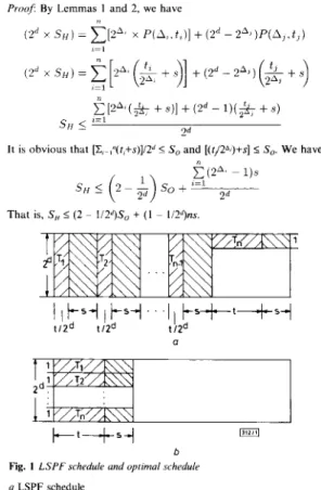
Fig. 1 LSPF schedule and optimal schedule a LSPF schedule
h Optimal schedule
Example: Let 1, = t and A, = d for i = I , 2, ._., 2 e l , and t,i = t and
A 2 d = 1. Fig. l a and b illustrate that the finish times of an LSDF
schedule and that of an optimal schedule are (21
+
2ds - f / z d ) and ( t+
s), respectively. Thus, S,, = (2 ~ 1/29So+
(2d - 2 -U29s
= (2 ~ 1/2”)So + ( I ~ l/2”)ns, where n = 2d,Corollary I : When the setup time is negligible, say s = dn, the worst performance bound of LSDF will approach (2 - 1/29 [6]. Acknowledgments: This research was supported by the National Science Council under grant NSC 83-0408EoO2-129.
0 IEE 1994
Electronics Letters Online No: 19941224
J.-F. Lin and S:J. Chen (Department of Electrical Engineering, National Taiwan University, Taiwan, Republic of China)
16 August 1994
References
DU. J., and LEUNG. J.Y.: ‘Complexity of scheduling parallel task systems’, SIAM J. Discrete Math.. 1989, 2, pp. 473487 MONMA, C.L., and pons. C.N.: ‘On the complexity of scheduling with batch setup times’, Operations Researches, 1989, 37, pp. 798-804 MONMA. c.L., and pons. c.N.: ’Analysis of heuristics for preemptive parallel machine scheduling with hatch setup times’, Operations Researches, 1993,41, (9, pp. 981-992
WANG, Q., and CHENG. K.H.: ‘A heuristic of scheduling parallel tasks and its analysis’, SIAM J. Cornput.. 1992, 21, (2). pp. 281-294 WONGINGER. G.J., and Yu. 2.: ‘A heuristic for preemptive scheduling with setup times’, Computing, 1992, 49, pp. 151-158
ZHU, Y., and AHUJA. M.: ‘On job scheduling on a hypercube’, IEEE Trans.. 1993, C-4, ( I ) , pp. 6 2 4 9
Efficient implementation
of
heuristic search
N. Cremelie and J.-P.
Martens
Indexing terms: Search problems. Arrificwl inrelligence
The heuristic search algorithm presented by Nilsson is commonly implemented with lists. However, the computational complexity of this implementation grows quadratically with the number of nodes being visited. The implementation presented has a computational complexity which is proportional to that number. Moreover, the storage requirements can be kept modest by introducing a late allocation strategy.
Introduction: Heuristic search is an attractive method for solving search problems. Instead of exhaustively investigating all possibili- ties, heuristic search relies on a best-first strategy: at any time the search proceeds in the direction that seems most likely to result in a solution. The decision of which path to examine first is based on heuristics.
Briej’ review of Nilsson algorithm: Search problems can be described as follows: given a set A of nodes, a set T of transitions between nodes, a set S c A of source nodes and a set G c A of goal nodes, find the path of successive transitions, starting in S and ending in
G,
exhibiting the smallest accumulation of transition costs. Nilsson [l] suggests ordering the nodes by means of an eval- uation functionf(n), estimating the cost of the best path from S to G passing through node n. The Nilsson algorithm uses two lists of nodes: an OPEN list of visited nodes still waiting for further expansion, and a CLOSED list of expanded nodes (‘expanding a node n’ means examining the transitions from n to its successor nodes). On initialisation, the source nodes are put in the OPEN list. Then the following sequence is executed repeatedly, until a stop criterion is reached(i) If OPEN is empty then stop the search (no solution!) else select from OPEN the node n with the smallest
An),
remove it from OPEN and put it in CLOSED. (ii)
if
n is a goal node then stop the search (solution found!) (iii) Expand n; for all successor nodes n, of n, computefln,), and:if
nj is not in OPEN nor CLOSED tben put n, in OPEN, store the path to n,else if the new Ani) < the old one then replace the old path to n, by the new one and put n, in OPEN.
Obviously, several list searches are required at each execution of the loop. Because the computational cost of searching in an unor- dered list is of the order p (the number of entries in the list), the above algorithm has a computational complexity of the order p2.
By sorting the lists, this complexity becomes proportional t o p log p .
1748
7 -
-
Implementation without lists: Suppose that the search space w n - sists of a finite set of N nodes, each having a unique index between 1 and N (assume that this index is easy to wmpute from the representation of the node). It is then possible to set up an array of N entries, with entry n containing all characteristics of node n:
An),
g(n), a hackpointer to the predecessor node, and a flag to indicate whether the node is open, closed or not yet visited. In this way, list searches are avoided. Information is now retrieved by an array indexing operation.a1
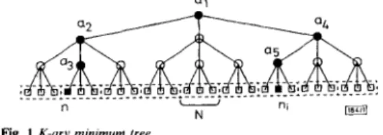
Fig. 1 K-ary minimum tree
The terminals 0 represent the search space nodes
To determine the open node having the smallest cost
An),
a K- ary tree is introduced. The nodes of the search space constitute the terminals of the tree (Fig. I ) and each non-terminal a holds a pointer to the best open node (terminal) reachable from a . Conse- quently, the root of the tree points to the best open node in the entire search space. It is useful to define the non-terminals on the branches connecting a terminal n with the root as the ‘ancestors’ of n. The ‘children’ of a non-terminal a are the K non-terminals or terminals on the branches leaving a .Initialising the tree is straightforward: all except the source nodes are new, the pointers in the source nodes’ ancestors are set appropriately, and the remaining non-terminals are set to point to some dummy node with an excessively high cost. Whenever a node changes in some way, only small portions of the tree need an update. Two cases can be distinguished:
Case I : Node n is selected f o r expansion and becomes closed Because n was the open node with the smallest fln). all ancestors of n ( a , , a?, a, in the case of Fig. I ) were referring to n and have to be updated as n becomes closed. The update process starts at the nearest ancestor of n ( a , in Fig. I): determine the minimum cost of the open nodes reachable from a, and let a , point to the node yielding this minimum. This requires K + a K tests, with
a
2 1 (always test on open status, test on cost if open). Updating the remaining ancestors of n ( a 2 , a , in Fig. I ) requires K ~ 1 tests for each ancestor: only the minimum cost of the terminals pointed to by its children is to be determined. Consequently, the total number of tests for this case is (K+
aK) + (K ~ 1) (log, N-
1) = TI.Case 2: The value o f J i n a successor n, of n is modified In this case, node n, becomes or remains open. The newfln,) must be compared to the costfin the nodes referred to by the ancestors of ni, starting at the nearest ancestor of n, and going up in the tree as long as the original cost was larger than fln,). The number of tests for this update is plog, N =
7
‘
,
(p
2 I).Case I occurs once per node expansion, whereas case 2 can apply for all successors. If the expected number of applications of case 2 is called y, then the total number of tests per expansion is given by T,(K)