國
立
交
通
大
學
網路工程研究所
碩
士
論
文
探勘使用者電器使用行為模式
Mining Usage Patterns from Appliance Data in Smart
Environment
研 究 生:柯宇倫
探勘使用者電器使用行為模式
Mining Usage Patterns from Appliance Data in Smart Environment
研 究 生:柯宇倫 Student:Yu-Lun Ko
指導教授:彭文志 Advisor:Wen-Chih Peng
國 立 交 通 大 學
網 路 工 程 研 究 所
碩 士 論 文
A ThesisSubmitted to Institute of Network Engineering College of Computer Science
National Chiao Tung University in partial Fulfillment of the Requirements
for the Degree of Master
in
Computer Science
September 2012
Hsinchu, Taiwan, Republic of China
探勘使用者電器使用行為模式 學生:柯宇倫 指導教授:彭文志 國立交通大學資訊科學與工程研究所 摘 要 最近幾年全球暖化的議題備受關注,而我們都知道說全球暖化是因為產生過量的 CO2和溫 室氣體所造成。根據研究,又以家中用電產生最多的溫室氣體,所以如果我們能節約家庭用 電,不僅可以減少溫室氣體的產生,相對也可以減少家庭用電的支出。但是節約用電對居住 者來說並不是一件簡單的任務,因為居住者無法獲得足夠的家庭用電資訊,居住者可以獲得 用電資訊的來源主要來自每個月的帳單或是家中的電表,但是居住者只能從帳單中知道總電 費或是從電表知道總耗電度數,即使看到帳單費用很貴,也無法做出有效且正確的決策在節 約用電上,使電費下降。因此我們在智慧家庭的環境下開發了一個系統,去分析居住者使用 電器的行為,這部份我們提出四種 usage pattern 去描述居住者使用電器的行為,所以當發 現這個月帳單比上個月高時,可以透過我們的系統知道他的用電資訊,更進一步還可以知道 是否有 extraordinary 的使用行為造成用電過高。 所以居住者可以透過我們的系統知道更多 的用電資訊,然後可以在節約用電的方面上做出有效率且正確的決策。此外我們利用真實智 慧家庭收集的資料去呈現我們所提出的四種 usage pattern。
ii
Mining Usage Patterns from Appliance Data in Smart Environment
Student: Yu-Lun Ko Advisors:Dr. Wen-Chih Peng
Institute of Computer Science National Chiao Tung University
ABSTRACT
In the last decade, considerable concern has arisen over the electricity saving due to the issue of reducing greenhouse gases. However, in daily lives, conserving electricity is not an easy task, since residents only can acquire the total electricity consumption from their bills or power meters. If more detailed behaviors of appliance usage are available, residents can make the correct policy to conserve the energy according to their frequent usage patterns. In this paper, based on four proposed usage patterns, we develop a system to analyze and aware users the detailed appliance usage information in a smart home environment. In advance, if the electricity cost is high, users can observe the extraordinary usage of appliances from the proposed system for energy saving easily. Furthermore, we also apply our system on real-world dataset to show the practicability of mining usage pattern in a smart home environment.
誌 謝
研究所兩年的時間過得很快,這兩年來在研究上遇到許多的困難,也學到了很多知識。 首先誠摯的感謝指導老師彭文志,老師讓我了解許多人生的道理、待人應有的應對進退,使 我這些年獲益匪淺。期許自己可以牢記這些寶貴的經驗,在未來的生活中能幫助自己迎接各 種挑戰。 本論文的完成亦得感謝博士班學長陳以錚的大力協助,及博士班學長朱文園和廖忠訓的 支持與鼓勵。因為有你們的體諒和陪伴,使得本論文能夠完整及嚴謹。 在碩士班的這兩年來,實驗室裡共同生活的點滴,學術上的討論、言不及義的閒扯、壓 力舒解的熱鬧聚餐、搞笑的機場接機,彷彿好像是昨日發生一樣,歷歷在目,也成為了我碩 士班這兩年的有趣回憶,感謝眾學長姐、同學、學弟妹的情義相挺,是你們讓兩年的研究生 活變得絢麗多彩。此外,感謝實驗室的博士班學長 Barry 學長、Oshin 學長、Dimension 學長 和博士後陳以錚學長們不厭其煩的指導與鼓勵,且總能在我迷惘時為我解惑。也感謝畢業碩 士班學長姐可愛的 Acrt Shen 學姊、有自己 schedule 的 Luc 學長、對事總是怡然自得的 KP、 時區在美國的小芊、投資很厲害的廷威學長的協助,而同屆的同學雅婷、拍拍、王堃瑋、Wallman 在大家互相幫忙之下,恭喜我們終於畢業了,你們的貼心及幫忙我銘感在心。當然最後不能 忘的還有可愛的學弟宗豪、永翔、凡凱、建志、守峻,謝謝你們這一年的陪伴跟幫忙 在口試的準備上,感謝老師及同學們在報告準備方面給於一些值得參考的建議與方向, 感謝陳以錚學長不厭其煩的幫我熬夜修改論文及投影片,也感謝學弟妹在口試當天的幫忙, 才使得口試可以順利進行。 最後,我也要特別感謝這兩年來家人的包容與鼓勵,媽媽、爸爸、弟弟,你們是我最大 的精神支柱,在我忙於碩士論文研究之餘,給予我很多的支持與鼓勵,我才能專心地做好研 究。 最後,謹以此文獻給我摯愛的你們。Contents
1 Introduction 1
2 Related Work 3
2.1 Energy Disaggregation and Appliance Recognition . . . 3
2.2 Time Series Similarity Function . . . 4
3 Preliminaries 5 4 Usage Pattern Analysis 7 4.1 Time Slot Usage Pattern . . . 7
4.2 Statistical Usage Pattern . . . 8
4.3 Clustered-based Statistical Usage Pattern . . . 11
4.4 Daily Behavior-based Usage Pattern . . . 12
5 Usage Alertion 15 5.1 System Architecture . . . 15
5.2 Extraordinary Usage Behavior for TS-UP . . . 16
5.3 Definition of Time Extraordinariness and Duration Extraordinariness for S-UP and CS-UP . . . 16
5.4 Definition of Daily Extraordinariness Usage Behavior for DB-UP . . . 17
6 Experimental Results 18 6.1 Data Sets . . . 18
6.2 Performance . . . 18
6.2.2 Discussion on S-UP Mining . . . 22 6.2.3 Discussion on CS-UP Mining . . . 26 6.2.4 Discussion on DB-UP Mining . . . 26
List of Figures
4.1 An example of the time slot usage pattern, S = 3, h = 8 . . . 8 5.1 System architecture for HAUBA . . . 15 6.1 TS-UP for each appliance . . . 19
6.2 Relation between extraordinary threshold and number of extraordinary usage
patterns for TS-UP . . . 20 6.3 Extraordinary TS-UP for each appliance . . . 21 6.4 Number of times to turn on the appliance . . . 23
6.5 Relation between extraordinary threshold and number of extraordinary usage
patterns for S-UP . . . 25
6.6 Relation between extraordinary threshold and number of extraordinary usage
patterns for CS-UP . . . 26 6.7 DB-UP for each appliance . . . 28
6.8 Relation between extraordinary threshold and number of extraordinary usage
patterns for DB-UP . . . 29 6.9 Extraordinary DB-UP for each appliance at γ = 200 . . . . 29
List of Tables
3.1 Sensor data format . . . 6
4.1 Notations of the time slot usage pattern . . . 8
4.2 An example of the statistical usage pattern . . . 10
4.3 Features of the similarity function . . . 14
6.1 Extraordinary threshold settings for each appliance . . . 20
6.2 S-UP for each appliance . . . 23
6.3 Threshold settings of S-UP for each appliance . . . 23
6.4 Extraordinary S-UP for each appliance . . . 24
6.5 CS-UP for each appliance . . . 25
Chapter 1
Introduction
Recently, concern over global climate change has motivated efforts to reduce the emissions of CO2 and other GHGs (greenhouse gases). Many researchers focus on the reduction of
elec-tricity usage, especially, the residential sector which is a significant contributor of greenhouse gases. With the consideration of electricity saving, people also can reduce the generation of GHGs. However, in general, it is difficult for residents to conserve the electricity, since, residents merely can obtain the information of total electrical cost from the bills or power meters. Residents usually do not know the electric consumption of each appliance in detail. If the electricity bill is expensive this month, we only can know it is expensive but do not know ”why” it is expensive. Hence, if more detailed behaviors of appliance usage are avail-able, residents can make the correct policy to conserve the energy more efficiently. Nowadays, due to the great progress of sensor technology, the data of all appliances in a house can be collected easily; however, extracting meaningful usage information is still a complex issue. The appliance usage behaviors usually vary with time; many behaviors of same appliances in summer and in winter are totally different. For example, the air-conditioner is usually turned on everyday in summer, but never turned on in other seasons. Different appliances may also have different usage behaviors; some appliances are seasonal-type and some ones are daily-type. For example, the air-conditioner usually is turned on in the summer but never turned on in other seasons, but the light usually is turned on and off frequently everyday. Obviously, how to extract meaningful usage pattern which can describe diversified appliance usage effectively and efficiently is really a challenging problem. Previous researches of usage patterns [8, 14, 15, 17, 18] mainly focused on energy disaggregation and appliance recognition.
To the best of our knowledge, few studies utilized the usage pattern to detect common or ex-traordinary user’s behavior for the target of energy saving. In this paper, a system, HAUBA (which stands for Household Appliance Usage Behavior Analysis), is developed to analyze and aware users the detailed appliance usage information in a smart home environment. We attach smart meters to all appliances in the smart home environment and setup a cloud server to collect usage data. From analyzing appliance data, we propose four types of usage pattern, time slot usage pattern (TS-UP), statistical usage pattern (S-UP), clustered-based statistical usage pattern (CS-UP), and daily behavior-based usage pattern (DB-UP), to represent and describe the appliance usage behavior effectively. We also propose four efficient algorithms for mining four types of usage patterns. Furthermore, we also have applied our system on real-world dataset to show the practicability of mining usage pattern in smart home environment. The contributions of this paper are as follows,
• From analyzing appliance usage data, four types of usage patterns are proposed to represent and describe the complex behaviors of appliance usage effectively. We also propose corresponding algorithms for mining four types of usage pattern efficiently. We also identify the extraordinary appliance usage behavior for each usage pattern.
• To the best of our knowledge, few studies have utilized the extraction of usage pattern for targeting the electricity conservation. In this paper, a system, HAUBA, is developed to provide usage time, usage duration, and significant appliance information for residents. We can make the correct policy to conserve the energy more efficiently.
The rest of the paper is organized as follows. Section 2 and Section 3 provide the related work and preliminary, respectively. Section 4 introduces the four types of usage pattern representation. Section 5 presents the proposed HAUBA system and discusses extraordinary pattern. Experimental results are given in Section 6. Finally, we conclude in Section 7.
Chapter 2
Related Work
In this section, we discuss some previous works utilized usage patterns for energy disag-gregation and appliance recognition, and some works about the similarity of extraordinary pattern.
2.1
Energy Disaggregation and Appliance Recognition
Hart [11] confirms how different electrical appliances generate distinct power consumption signatures, which often could be seen in the aggregated power load. He shows how on-off events characterize the use of some appliances enough. For other appliances, Hart considers using finite state machines to find features. Hart names this approach nonintrusive appli-ance load monitoring(NALM). Farinaccio et al. [8] used the pattern, such as, number of data point and ON-OFF switch, to disaggregate whole-house electricity consumption into its ma-jor end-uses. Suzuki et al. [20] use new NIALM technique based on integer programming to disaggregate residential power use. Lin et al. [17] used a dynamic Bayesian network and filter to disaggregate the data online. Kim et al. [15] investigated the effectiveness of sev-eral unsupervised disaggregation methods on low frequency power measurements collected in real homes. Author proposed a usage pattern which consists on-duration distribution and dependency between appliances. Goncalves et al. [10] explored an unsupervised approach to determine the number of appliances in the household, including their power consumption and state, at any given moment. Chen et al. [?] disaggregated utility consumption from smart meters into specific usage that associated with human activities. Authors proposed a novel
statistical framework for disaggregation on coarse granular smart meter readings by modeling fixture characteristic, household behavior, and activity correlations.
Prudenzi [19] utilized an artificial neural network based procedure for identifying the elec-trical signatures of residential appliances. Ito et al. [13] extract features from the current (e.g., amplitude, form, timing) to develop appliance signatures. For appliance recognition, Kato et al. [14] used Principal Component Analysis to extract features from electric signals and classified them by Support Vector Machine. Aritoni et al. [1] propose a software pro-totype which can be used to understand the household appliances behavior. Some of these works and the characteristics of workable solutions were discussed by Matthews et al. [18].
2.2
Time Series Similarity Function
There are existing time series similarity measuring methods, such as Euclidean distance, DTW [3], LCSS [21], EDR [5], ERP[4] and many other proposed novel methods. According to the experimental survey in Querying and Mining of Time Series Data: Experimental Com-parison of Representations and Distance Measures [7], the conclusion is that elastic measuring methods such as DTW , LCSS, EDR and ERP are significantly more accurate than lock-step methods like Lp-norms and DISSIM [9] when the data set is not huge. Moreover, the elas-tic measuring methods also generally outperforms some novel methods(TQuEST [2], SpADe [6])in accuracy. For comparison between the elastic measuring methods, the experimental results also show that the edit distance based methods like LCSS, EDR and ERP in fact have very close accuracy compared to DTW. Based on this conclusion in [7], we implement DTW, EDR and LCSS for our time series data similarity measuring.
Chapter 3
Preliminaries
The input data in our algorithms is usage log of an appliance. The usage log of an appliance
k is Uk, each in form of Uk=< D1k, D2k, ..., DN k>, where Dik refers to daily log for appliance
k and the Dik is stream of sensor events, each in form of e =< s, t, c, p >, where s refers
to a sensor ID and t refers to the timestamp when sensor s has been activated. Then, the value of c represents a status of appliance k. There are two values for c. One of the values is 1 which represents the appliance turns ON and the other value is 0 which represents the appliance turns OFF. Finally, the p refers to the current power consumption. The Table 3.1 shows an example about a sensor event. Therefore, the Dik is a sequence of r sensor events
< e1, e2, ..., er >. After we obtain the usage log of an appliance k, we extract four types usage
pattern and identify the extraordinary usage behavior from usage log for the appliance k. The related terms and definition are summarized below, and will be used in the rest of the paper. In the next section, we will introduce how to extract the usage pattern and identify the extraordinary usage behavior.
Definition 1. Start Time: Given stream of sensor events < e1, e2, ..., er > for a day. If
cj in ej is ON and ci in ei is OFF where j < i≤ r, we say that the tj is start time.
Definition 2. Duration: Given stream of sensor events < e1, e2, ..., er> for a day. If cj
in ej is ON and ci in ei is OFF where j < i≤ r, the duration dj is ti− tj.
Definition 3. Usage Point: Given N days start time set < t11, t12, K, tN j > and N
days duration set < d11, d12, ..., dN j >. A usage point is a pair < tij, dij >. The tij represents the jth time to turn on the appliance in the ith day and the dij represents the duration of the jth time to turn on the appliance in the ith day. In the statistical usage pattern (S-UP)
Table 3.1: Sensor data format
sensor ID time status power consumption
2 2011/3/14 20:00:00 1 58W
and clustered-based statistical usage pattern (CS-UP), the usage point is a type of behavior to turn on the appliance.
Definition 4. Appliance Time Series Data: The Appliance Time Series Data A
is sequence of status of appliance, with each value ai sampled at a specific point ti, i.e;
Chapter 4
Usage Pattern Analysis
In this section, we will introduce the four usage patterns. The section 4.1 introduces the time slot usage pattern (TS-UP) and the section 4.2 introduces statistical usage pattern (S-UP). After introducing the S-UP and TS-UP, the section 4.3 and 4.4 introduce clustered-based statistical usage pattern (CS-UP) and daily behavior-based usage pattern (DB-UP).
4.1
Time Slot Usage Pattern
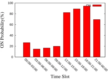
For extracting time slot usage pattern (TS-UP), we partitions each day into h time slots and each time slot size is S. Then, we evaluate ON probability of each time slot for N days data. The usage duration U Dij (the jth slot in the ith day) is summed together, divided by total slot time in the jthslot which is time slot size S multiplied by N . For example, the time slot size S is 3 hours, so the number of time slots h is 8 (i.e., 24/3 =8). The time slots are 0 : 00 ∼ 03 : 00, 03 : 00 ∼ 06 : 00, 6 : 00 ∼ 09 : 00 ...etc. Evaluating the ON probability of the first time slot, we sum the usage duration U Di1, where the i is from 1 to N . Then, the summation is divided by 3*N . The equation of ON probability is
Pj(ON ) =
∑N
i=1U Di,j
T otal Slot T ime, j = 1, 2, 3..., h (1)
The Table 4.1 shows the some symbols and the meaning of the symbols. Specifically, the extracting algorithm is described in Algorithm 1. In the Algorithm 1, the Get T otal Duration function computes the total duration of the jthtime slot in the ith day. So the first parameter
0 20 40 60 80 100 00:00-03:0003:00-06:0006:00-09:0009:00-12:0012:00-15:0015:00-18:0018:00-21:0021:00-00:00 ON Probability(%) Time Slot ON
Figure 4.1: An example of the time slot usage pattern, S = 3, h = 8
Table 4.1: Notations of the time slot usage pattern
symbols meaning
h Number of time slots
N Number of days data
S Time slot size
U Dij The total duration of the jth time slot in the ith day
Pj(ON ) The ON probability of the jthtime slot
for the Get T otal Duration function is the ith day data and the second parameter is the jth time slot. So the function Get T otal Duration can get the total duration of the jth time slot in the ith day, that is U Dij. To evaluate the total duration of the jth time slot for N days data, we sum the U Dij for each i and record the result in the Slot Durationj. Finally, we evaluate the Pj(ON ) by Slot Durationj divided by S multiplied by N . The Figure 4.1 shows an example of time slot usage pattern.
The TS-UP can provide the information about that the appliance is turned on frequently at which time slot and the usage duration of each time slot. But it can’t provide exact time that the appliance is turned on and the duration. So we propose the statistical usage pattern (S-UP) which is introduced in next section.
Algorithm 1: Time Slot Usage Pattern Extracting Algorithm
Input: Usage log Uk =< d1k, d2k, ..., dN k >, time slot size S
Output: Probability of turning on the appliance k for each time slot
P1(ON ), P2(ON ), ..., Ph(ON )
h← 24/S; 1 for i = 1→ N do 2 for j = 1→ h do 3
U Dij ← Get T otal Duration(Dik, j);
4
for j = 1→ h do
5
for i = 1→ N do
6
Slot Duration[j]← Slot Duration[j] + UDij;
7
for j = 1→ h do
8
Pj(ON )← Slot Duration[j]/(S × N);
9
return P1(ON ), P2(ON ), ..., Ph(ON );
10
on appliance, the third time to turn on appliance... etc. Then, we evaluate how many days there are the behaviors of the jth time to turn on the appliance and we use mj to represent it. Then, we check the mj whether it is larger than or equal to minimum support ρ∗ N. If it is smaller than ρ∗ N, it will be removed. Because we think it is a infrequent behavior. After above step, we evaluate the mean of the start time µ(tj) for each jth time to turn on the appliance and also evaluate the mean of the usage duration µ(dj) for N days data. The equation of evaluating mean of the start time for each jth time to turn on the appliance is
µ(tj) =
∑N
i=1tij
mj
, j = 1, 2, 3... (2)
and the equation of evaluating mean of the usage duration for the jth time to turn on the appliance is µ(dj) = ∑N i=1dij mj , j = 1, 2, 3... (3)
The extracting algorithm is described in Algorithm 2. In Algorithm 2, we use the Get M aximum T ime function to get the maximum j which represents the jth time to turn on the appliance. After
getting the maximum j, we count number of days for each time to turn on the appliance by Count Each T ime function and record the value to N umber of Days[j]. To Remove the infrequent behavior of turn on the appliance, we compare the N umber of Days[j] with ρ∗ N and record remaining usage points to Ur. Then, we use the Get M aximum T ime function to
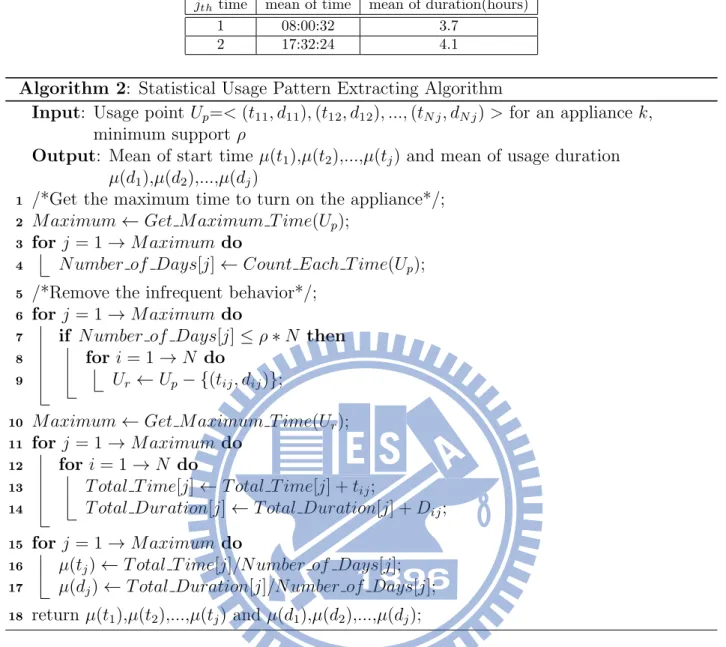
Table 4.2: An example of the statistical usage pattern
jth time mean of time mean of duration(hours)
1 08:00:32 3.7
2 17:32:24 4.1
Algorithm 2: Statistical Usage Pattern Extracting Algorithm
Input: Usage point Up=< (t11, d11), (t12, d12), ..., (tN j, dN j) > for an appliance k,
minimum support ρ
Output: Mean of start time µ(t1),µ(t2),...,µ(tj) and mean of usage duration
µ(d1),µ(d2),...,µ(dj)
/*Get the maximum time to turn on the appliance*/;
1
M aximum← Get Maximum T ime(Up);
2
for j = 1→ Maximum do
3
N umber of Days[j]← Count Each T ime(Up);
4
/*Remove the infrequent behavior*/;
5
for j = 1→ Maximum do
6
if N umber of Days[j]≤ ρ ∗ N then
7
for i = 1→ N do
8
Ur ← Up− {(tij, dij)};
9
M aximum← Get Maximum T ime(Ur);
10
for j = 1→ Maximum do
11
for i = 1→ N do
12
T otal T ime[j]← T otal T ime[j] + tij;
13
T otal Duration[j]← T otal Duration[j] + Dij;
14
for j = 1→ Maximum do
15
µ(tj)← T otal T ime[j]/Number of Days[j];
16
µ(dj)← T otal Duration[j]/Number of Days[j];
17
return µ(t1),µ(t2),...,µ(tj) and µ(d1),µ(d2),...,µ(dj);
18
get the new maximum j from Ur. To evaluate the mean of start time µ(tj) and mean of usage duration µ(dj), We use T otal T ime[j] divided by N umber of Days[j] and T otal Duration[j] divided by N umber of Days[j]. The example of statistical usage pattern is like Table 4.2. However, we think that the mean value will be affected by the noise data easily and find that
4.3
Clustered-based Statistical Usage Pattern
The clustered-based statistical usage pattern (CS-UP) is a usage pattern which improves the S-UP. The difference between S-UP and CS-UP is that CS-UP distinguishes user behaviors and remove the noise data from the jth time to turn on the appliance before evaluating the mean of start time and the mean of the duration for the jth time to turn on the appliance. So the CS-UP clusters the similar behavior (close time and close duration) and removes noise data in the jth time to turn on the appliance. The clustering method we used is the agglomerative hierarchical clustering algorithm. The agglomerative hierarchical clustering algorithm has two optimal efficient approach, single-linkage and complete-linkage. In our work, we use the single-linkage approach. After deciding the clustering algorithm, we do two phases of clustering. The first phase of clustering is by the start time and the second phase of clustering is by the duration. For the first phase, each usage point is a cluster and merges the closest usage point which has the closest start time. In other words, the distance of start time which is smaller than or equal to time threshold σ will be merged first. Then, we merge the cluster repeatedly until the distance of start time between cluster and the other cluster is not smaller than or equal to σ. After the first phase clustering, we do the clustering on the existing clustering results by their durations for the second phase. Like the first phase, we also merge the cluster which has the closest duration. The closest duration means the distance of duration which is smaller than or equal to duration threshold ϵ. After doing two phases of clustering, we have many clusters for the jth time to turn on the appliance and each cluster represents a behavior of the the jth time to turn on the appliance. Finally, we select a maximum cluster to represent the behavior of the jth time to turn on the appliance. Specifically, this extracting algorithm is described in Algorithm 3. In the Algorithm 3, the first step is like the S-UP to remove infrequent behaviors. Then, using Hierarchical Clustering function clusters the similar usage points by start time and store the result to CTj. Then, we use Hierarchical Clustering function to cluster by duration for each cluster in CTj and store the result to the CDj. After getting the CDj, we use Get M aximum Cluster function to get the maximal cluster to represent behavior of jth time to turn on the appliance and store the result to the Cj. Then, we evaluate centroid of the cluster to represent Cj by
Algorithm 3: Clustered-based Statistical Usage Pattern Extracting Algorithm
Input: N days usage point Up=< (t11, d11), (t12, d12), ..., (tN j, dN j) > for an appliance
k, minimum support ρ, time threshold σ, duration threshold ϵ
Output: Centroid of cluster < µ(t1), µ(d1) >, < µ(t2), µ(d2) >, ..., < µ(tj), µ(dj) >
/*Get the maximum time to turn on the appliance*/;
1
M aximum← Get Maximum T ime(Up);
2
for j = 1→ Maximum do
3
N umber of Days[j]← Count Each T ime(Up);
4
/*Remove the infrequent behavior*/;
5
for j = 1→ Maximum do
6
if N umber of Days[j]≤ ρ ∗ N then
7
for i = 1→ N do
8
Ur ← Up− {(tij, dij)};
9
M aximum← Get Maximum T ime(Ur);
10 for j = 1→ Maximum do 11 /*Cluster by time*/; 12 CTj ← {Hierarchical Clustering(Ur, j, σ)}; 13
N umber of Clusters[j]← Get Number of Clusters(CTj);
14
/*Cluster by duration*/;
15
for i = 1→ Number of Clustersj do
16
CDj ← CDj ∪ {Hierarchical Clustering(CTj, i, ϵ)};
17
Cj ← Get Maximum Cluster(CDj);
18 for j = 1→ Maximum do 19 < µ(tj), µ(dj) >← Evaluate Centroid(Cj); 20 return < µ(t1), µ(d1) >, < µ(t2), µ(d2) >, ..., < µ(tj), µ(dj) >; 21
4.4
Daily Behavior-based Usage Pattern
For extracting daily behavior-based usage pattern (DB-UP), we consider a daily log as a behavior and we discover that some daily usage behaviors are similar. Because we want to find representative daily usage behaviors from daily usage logs, we make similar daily usage behavior in the same group. We find that the daily usage log is daily appliance time series data and its y axis just has two values (1 or 0). For making similar appliance time series data
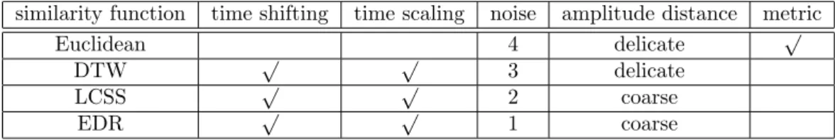
can be said that a time series distance qualifies the distance between the sequences of time series data as points in the clustering space. Based on the observation in [7], which was also described in the related works section, we chose to implement elastic measuring methods DTW, LCSS, EDR for our appliance time series data distance function. One important point about appliance time series data is that time shifting constrain needs to be added when applying elastic measuring methods. That is, the range of local time shift should be limited. In our case, we think even though two appliance time series data have a little time shifting, they are also similar. This is an intuitive reason. We define the time shifting constrain as ω. For example, if we set ω=30(minutes), the similarity of any two elements form the two sequences can be counted only when their time distance is still below 30 minutes.
Among the three methods, DTW was first proposed as an elastic distance function that aims to find the optimal alignment between two time series sequences because the earliest method, Euclidean distance, has been found to be very weak at handling noise and local time shifting. DTW can handle local time shifting, but is still sensitive to noise. Later, LCSS and EDR were proposed to measure similarity of usage behavior allowing the skipping of some points to match similar common subsequences. In this work, we want to find the similarity function that can deal with local time shifting under a time shifting constrain, and can which deal with noise, but which does not allow too much amplitude shifting. Based on the observation in [7], we first list the feature table which compares four similarity function. The Table 4.3 shows features of the four similarity functions. In the Table 4.3, the number is the bigger for the column ”noise”, the similarity function is the more sensitive for the noise. Because the EDR is the best similarity function for handling noise, we choice it to be our similarity function. After getting the similarity score, we cluster these appliance time series data. At first, we use the SHRINK [12] which is parameter-free network clustering algorithm. But it will find the hubs. The hub is the node which doesn’t in any clusters, but it is overlapped by more than two clusters. In out work, the hub means a daily usage log has property of two representative daily behaviors. But we think a daily usage log just has property of a behavior. So we use the agglomerative hierarchical clustering algorithm. It is introduced in section 4.3. At first, each daily appliance time series data is a cluster and we merge two daily appliance time series data whose similarity is the smallest and smaller than η. After the merging, we need to modify the similarity score between new cluster and another
Table 4.3: Features of the similarity function
similarity function time shifting time scaling noise amplitude distance metric
Euclidean 4 delicate √
DTW √ √ 3 delicate
LCSS √ √ 2 coarse
EDR √ √ 1 coarse
cluster. We do this step repeatedly until the similarity score between cluster and cluster is not smaller than η. After getting the results of clustering, we compute mean of the cluster to represent cluster. Specifically, the extracting algorithm is described in Algorithm 4. In the Algorithm 4, we evaluate the similarity of the daily appliance time series data for each other by the EDR and store to Similarityij at first. Based on the similarity, we do the hierarchical clustering algorithm to cluster the daily usage behavior which the similarity score is smaller than or equal to η. After the clustering, we get the results C1, C2, ..., Cn and evaluate the centroid of the each cluster Ci. The set of centroid of each cluster is {R1, R2, ..., Rn}. The Ri
represent the one of the daily behaviors.
Algorithm 4: Daily Behavior-based Usage Pattern Extracting Algorithm
Input: Usage log Uk =< D1k, D2k, ..., FN k > for an appliance k, similarity threshold η;
Output: Centroid of clusters{R1, R2, ..., Rn}
for i = 1→ N do 1 for j = 1→ N do 2 Similarityij ← EDR(Dik, Dj k); 3
{C1, C2, ..., Cn} ← Hierarchical Clustering(Uk, Similairty, η);
4 for i = 1→ N do 5 Ri ← Evaluate Centroid(Ci); 6 return{R1, R2, ..., Rn}; 7
Chapter 5
Usage Alertion
5.1
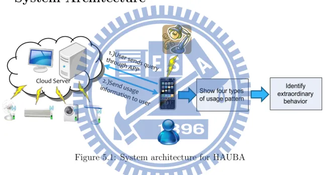
System Architecture
Figure 5.1: System architecture for HAUBA
The architecture of proposed system is shown in Figure 5.1. We attach wireless power meters to all appliances in the smart home environment and setup a cloud server to collect usage data. Power meters will send the log data of appliance to server every constant time (about 3 to 4 seconds). When a user wants to know the information of an appliance, he/she can use the smart phone connect to cloud server and check the usage behavior (four types usage pattern which are introduced in chapter 4). Furthermore, if the electricity bill is high this month, users can observe the extraordinary usage of appliances comparing with the discovered pattern from the proposed system. User can modify the range of parameter setting to control the tolerance of extraordinary usage behavior (i.e., the number of generated extraordinary
patterns). The definition of extraordinary usage behavior will be introduced in next section.
5.2
Extraordinary Usage Behavior for TS-UP
To identify the new behavior Bnew whether it is extraordinary, we extract the TS-UP for the normal behavior Bnor mal and the its TS-UP is P1(ON ),P2(ON ),..., Ph(ON ). For the new behavior, we also extract TS-UP which is E1(ON ), E2(ON ), ..., Eh(ON ). Then, we evaluate the Sa which is the score of extraordinariness. The equation 1 describes the method of evaluating Sa. If Sa is larger than extraordinary threshold δ, we say that the Bnew is extraordinary. Otherwise, it is normal.
Sa=
h ∑
i=1
| Pi(ON )− Ei(ON ) | (1)
5.3
Definition of Time Extraordinariness and Duration
Extraordinariness for S-UP and CS-UP
To identify the new behavior Bnew whether it is extraordinary, we extract the S-UP or CS-UP for the normal behavior Bnor mal and the its S-UP or CS-UP is < µ1(Tstar t), µ1(Dusag e) >
, < µ2(Tstar t), µ2(Dusag e) >, ..., < µj(Tstar t), µj(Dusag e) >. For the new behavior, we also
extract S-UP or CS-UP which is < µ1( ˆTstar t), µ1( ˆDusag e) >, < µ2( ˆTstar t), µ2( ˆDusag e) >, ..., < µj( ˆTstar t), µj( ˆDusag e) >. Then, we evaluate the St and Sd which are the score of time ex-traordinariness and score of duration exex-traordinariness. The equation 2 and 3 describe the method of evaluating St and Sd. If St is larger than extraordinary time threshold α, we say that the Bnew is time extraordinariness. If Sd is larger than extraordinary duration threshold
β, we say that the Bnew is duration extraordinariness. If Bnew is not time extraordinariness
5.4
Definition of Daily Extraordinariness Usage
Behav-ior for DB-UP
To identify the new behavior Bnew whether it is extraordinary, we extract the DB-UP for the normal behavior Bnor mal and its DB-UP is RBnor mal = {R1, R2, ..., Rm}. For the new
behavior, we also extract DB-UP which is RBnew = {Q1, Q2, ..., Qn}. Then, we select the
element from RBnew in the order at first and each of the elements finds the similar element from RBnor mal. Because element of RBnor mal and RBnew are appliance time series data, we can use time series similarity function which is introduced in section 4.4 to measure their similarity. If one of the elements in RBnew can’t find a similar element in RBnor mal, the
RBnew is extraordinary. In other words, the score of similarity between one of elements Qj
and all elements of RBnor mal is larger than γ, the RBnew is extraordinary. Otherwise, it is normal.
Chapter 6
Experimental Results
In this section, we introduce our dataset in the section 6.1 and we discuss with four types of usage pattern and parameter settings of extraordinary usage behavior in the section 6.2.
6.1
Data Sets
The real data set we used is collected by [16]. There are microwave, dish-washer, wash-dryer, light, oven and air-conditioned. For each appliance, they collect the data for three years and the sample rate is about 3 or 4 seconds. So a day has about 22550 data points.
6.2
Performance
As mentioned in the previous chapter, we propose four usage patterns and identify what the extraordinary usage behavior is. In this section, we will show the normal usage pattern
which we extract and threshold settings. Therefore, for each appliance, we use the first
year data to be the normal behavior and extract its four types of usage pattern. Then, we divide the remaining two years data into 24 months and they are 24 new behaviors. We
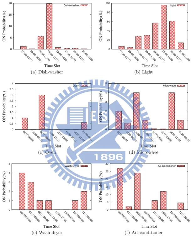
we set η to 400 which is the similarity threshold for DB-UP and set time threshold σ to 15 minutes and duration threshold ϵ to 30 minutes in our experiment. We discuss the detail below. 0 5 10 15 20 00:00-03:0003:00-06:0006:00-09:0009:00-12:0012:00-15:0015:00-18:0018:00-21:0021:00-00:00 ON Probability(%) Time Slot Dish-Washer (a) Dish-washer 0 20 40 60 80 100 00:00-03:0003:00-06:0006:00-09:0009:00-12:0012:00-15:0015:00-18:0018:00-21:0021:00-00:00 ON Probability(%) Time Slot Light (b) Light 0 0.5 1 1.5 2 2.5 3 3.5 4 00:00-03:0003:00-06:0006:00-09:0009:00-12:0012:00-15:0015:00-18:0018:00-21:0021:00-00:00 ON Probability(%) Time Slot Oven (c) Oven 0 1 2 3 4 5 00:00-03:0003:00-06:0006:00-09:0009:00-12:0012:00-15:0015:00-18:0018:00-21:0021:00-00:00 ON Probability(%) Time Slot Microwave (d) Microwave 0 1 2 3 4 5 00:00-03:0003:00-06:0006:00-09:0009:00-12:0012:00-15:0015:00-18:0018:00-21:0021:00-00:00 ON Probability(%) Time Slot Wash-Dryer (e) Wash-dryer 0 5 10 15 20 25 30 00:00-03:0003:00-06:0006:00-09:0009:00-12:0012:00-15:0015:00-18:0018:00-21:0021:00-00:00 ON Probability(%) Time Slot Air-Conditioner (f) Air-conditioner Figure 6.1: TS-UP for each appliance
0 5 10 15 20 25 61 51 41 31 21 11 1 0 20 40 60 80 100 120 140
# of extraordinary usage patterns # of extraordinary usage patterns
extraordinary threshold δ microwave light dish-washer air-conditioner wash-dryer oven total extraordinary usage patterns
Figure 6.2: Relation between extraordinary threshold and number of extraordinary usage patterns for TS-UP
Table 6.1: Extraordinary threshold settings for each appliance appliance name range of δ (%)
microwave 0.6∼ 4 light 16∼ 56 air-conditioner 4∼ 56 oven 0.6∼ 7 dish-washer 4∼ 16 wash-dryer 2∼ 13
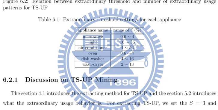
6.2.1
Discussion on TS-UP Mining
The section 4.1 introduces the extracting method for TS-UP and the section 5.2 introduces what the extraordinary usage behavior is. For extracting TS-UP, we set the S = 3 and N = 365. The Figure 6.1 shows the TS-UP for each appliance. Comparing each TS-UP for different appliances, we can easily see that they have different high usage frequency at different time slot and they have different probability for each time slot. Based on our extracting method, we also can say they have different usage duration for each time slot. For example,
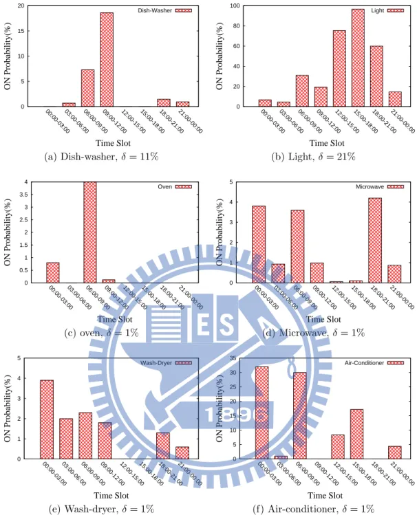
0 5 10 15 20 00:00-03:0003:00-06:0006:00-09:0009:00-12:0012:00-15:0015:00-18:0018:00-21:0021:00-00:00 ON Probability(%) Time Slot Dish-Washer (a) Dish-washer, δ = 11% 0 20 40 60 80 100 00:00-03:0003:00-06:0006:00-09:0009:00-12:0012:00-15:0015:00-18:0018:00-21:0021:00-00:00 ON Probability(%) Time Slot Light (b) Light, δ = 21% 0 0.5 1 1.5 2 2.5 3 3.5 4 00:00-03:0003:00-06:0006:00-09:0009:00-12:0012:00-15:0015:00-18:0018:00-21:0021:00-00:00 ON Probability(%) Time Slot Oven (c) oven, δ = 1% 0 1 2 3 4 5 00:00-03:0003:00-06:0006:00-09:0009:00-12:0012:00-15:0015:00-18:0018:00-21:0021:00-00:00 ON Probability(%) Time Slot Microwave (d) Microwave, δ = 1% 0 1 2 3 4 5 00:00-03:0003:00-06:0006:00-09:0009:00-12:0012:00-15:0015:00-18:0018:00-21:0021:00-00:00 ON Probability(%) Time Slot Wash-Dryer (e) Wash-dryer, δ = 1% 0 5 10 15 20 25 30 35 00:00-03:0003:00-06:0006:00-09:0009:00-12:0012:00-15:0015:00-18:0018:00-21:0021:00-00:00 ON Probability(%) Time Slot Air-Conditioner (f) Air-conditioner, δ = 1% Figure 6.3: Extraordinary TS-UP for each appliance
evaluate the Sa by comparing the first year TS-UP with each month TS-UP. If the Sa is larger than extraordinary threshold δ, we say the usage behavior of that month is extraordinary. The Figure 6.2 shows the number of extraordinary usage behaviors for different appliances at different values of δ. We can see that different appliances have different range of extraordinary threshold settings. For example, the extraordinary threshold of microwave is range from 0.6%
to 4% and the light is range from 16% to 60%. It reveals that the definition of extraordinary usage behavior for microwave is different from the light, because they have different usage behavior. The Table 6.1 shows the δ value setting for each appliance. The Figure 6.3 shows one of extraordinary usage patterns for each appliance.
6.2.2
Discussion on S-UP Mining
The method of extracting S-UP is introduced in section 4.2. For the S-UP, we need
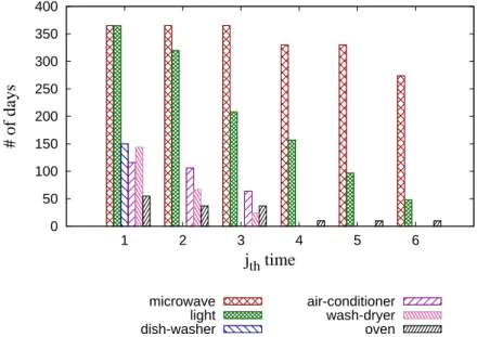
to discuss how to set minimum support ρ,time extraordinariness threshold α, and duration extraordinariness threshold β. We evaluate each time for a year and the result of evaluation is showed by Figure 6.4. As shown in Figure 6.4, residents turn on the light and microwave every day and at most turn on six times a day. The microwave has 274 days to turn on six times a day among a year and the light have 48 days to turn on six times a day. The dish-washer has 150 days to turn on once a day and it doesnt have a day to turn on more than twice. Then, the air-conditioned and wash-dryer turn on at most third times a day. Following the results of Figure 6.4, we can set the ρ larger than 1% and smaller than 16%. Because we set the ρ for 16% (58.4 days), the usage behavior of oven will be removed. Therefore, we set the ρ for 10% (36.5 days) in this experiment. After setting the ρ, we use this ρ to extract S-UP for normal behavior. The Table 6.2 shows S-UP for each appliance. The Table 6.2 shows normal S-UP for each appliance. The relation between time extraordinariness threshold and number of extraordinary usage patterns is illustrated in Figure 6.5a, where wash-dryer, light, microwave, and air-conditioned set time threshold for 1 hour to 11 hours, and the oven and the dish-washer set time threshold for 1 second to 3 hours. Figure 6.5b shows the relation between duration extraordinariness threshold β and number of extraordinary usage patterns. We can see the range of β for each appliance is different. The β of microwave sets for 0.05 hours to 0.15 hours and the β of dish-washer and wash-dryer set for 0.05 hours to 0.3 hours.
0 50 100 150 200 250 300 350 400 1 2 3 4 5 6 # of days jth time microwave light dish-washer air-conditioner wash-dryer oven
Figure 6.4: Number of times to turn on the appliance Table 6.2: S-UP for each appliance
appliance name jth time mean of time mean of duration(hours)
microwave 1 05:00:00 0.06 2 08:00:00 0.05 3 10:00:00 0.05 4 11:00:00 0.046 5 13:00:00 0.03 6 14:00:00 0.032 light 1 05:00:00 5.1 2 11:00:00 4.11 3 13:00:00 1.80 4 14:00:00 3.268 5 16:00:00 1.4 6 13:00:00 1.65 wash-dryer 1 11:00:00 0.65 2 08:00:00 0.49 dish-washer 1 08:00:00 2.08 oven 1 05:00:00 0.72 2 13:00:00 0.2 3 13:01:00 0.12 air-conditioner 1 02:00:00 7.48 2 15:00:00 3.22 3 20:00:00 1.56
Table 6.3: Threshold settings of S-UP for each appliance appliance name range of α (hours) range of β (hours)
microwave 1∼ 11 0.05∼ 0.15 Light 1∼ 11 5∼ 13 air-conditioner 1∼ 11 0.25∼ 0.5 oven 1∼ 3 0.05∼ 0.65 dish-washer 1∼ 3 0.05∼ 0.3 wash-dryer 1∼ 11 0.05∼ 0.3
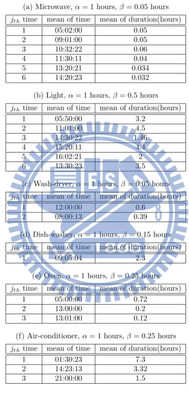
Table 6.4: Extraordinary S-UP for each appliance (a) Microwave, α = 1 hours, β = 0.05 hours jth time mean of time mean of duration(hours)
1 05:02:00 0.05 2 09:01:00 0.05 3 10:32:22 0.06 4 11:30:11 0.04 5 13:20:21 0.034 6 14:20:23 0.032
(b) Light, α = 1 hours, β = 0.5 hours jth time mean of time mean of duration(hours)
1 05:50:00 3.2 2 11:01:00 4.5 3 14:30:22 1.46 4 15:20:11 4.4 5 16:02:21 2 6 13:30:23 3.5
(c) Wash-dryer, α = 1 hours, β = 0.05 hours jth time mean of time mean of duration(hours)
1 12:00:00 0.6
2 08:00:13 0.39
(d) Dish-washer, α = 1 hours, β = 0.15 hours jth time mean of time mean of duration(hours)
1 09:05:04 2.3
(e) Oven, α = 1 hours, β = 0.25 hours jth time mean of time mean of duration(hours)
1 05:00:00 0.72
2 13:00:00 0.2
3 13:01:00 0.12
(f) Air-conditioner, α = 1 hours, β = 0.25 hours jth time mean of time mean of duration(hours)
0 5 10 15 20 25 11 9 7 5 3 1 0 20 40 60 80 100 120 140
# of extraordinary usage patterns # of extraordinary usage patterns
time extraordinariness threshold α (hours) microwave light dish-washer air-conditioner wash-dryer oven total extraordinary usage patterns
(a) Time extraordinariness threshold
0 5 10 15 20 25 0.55 0.45 0.35 0.25 0.15 0.05 0 20 40 60 80 100 120 140
# of extraordinary usage patterns # of extraordinary usage patterns
duration extraordinariness threshold β (hours) microwave light dish-washer air-conditioner wash-dryer oven total extraordinary usage patterns
(b) Duration extraordinariness threshold Figure 6.5: Relation between extraordinary threshold and number of extraordinary usage patterns for S-UP
Table 6.5: CS-UP for each appliance appliance Name centroid of cluster
jth time mean of time mean of duration(hours)
microwave 1 02:57:37 0.02 2 04:11:09 0.05 3 06:30:34 0.03 4 06:35:47 0.05 5 06:39:02 0.02 6 07:03:47 0.08 light 1 00:00:00 11.02 2 07:29:06 12 3 20:20:11 0.05 4 21:34:39 1.14 5 21:08:44 1.37 6 09:54:52 0.6 wash-dryer 1 00:02:11 0.63 2 23:59:32 0.52 dish-washer 1 08:33:55 2.19 oven 1 06:51:39 0.78 2 22:39:22 0.22 3 23:08:09 0.173 air-conditioner 1 00:00:02 9 2 22:00:01 2 3 23:00:01 1
6.2.3
Discussion on CS-UP Mining
We know the CS-UP is improved method for S-UP. Therefore, it also has minimum support ρ, time extraordinariness threshold α, and duration extraordinariness threshold β. At first, the setting of ρ is the same as S-UP and we also extract the CS-UP. At first, the setting of ρ is the same as S-UP. The Table 6.5 shows the normal CS-UP for each appliance. Then, we discuss with setting α and β. As shown in Figure 6.6a and 6.6b, we can see all of the appliances have in the same range of α. The range of α is from 0.4 hours to 1 hours. For the β, only the β range of microwave is from 2 minutes to 7 minutes and the others are from 2 minutes to 32 minutes. Because we use the clustering method to make each month jth time start time and duration close to the normal behavior, the range of time extraordinariness threshold and duration extraordinariness isn’t dispersion. The Table 6.6 shows the extraordinary CS-UP for each appliance. 0 5 10 15 20 25 1 0.9 0.8 0.7 0.6 0.5 0.4 0 20 40 60 80 100 120 140
# of extraordinary usage patterns # of extraordinary usage patterns
time extraordinariness threshold α (hours) microwave light dish-washer air-conditioner wash-dryer oven total extraordinary usage patterns
(a) Time extraordinariness threshold
0 5 10 15 20 25 32 27 22 17 12 7 2 0 20 40 60 80 100 120 140
# of extraordinary usage patterns # of extraordinary usage patterns
duration extraordinariness threshold β (hours) microwave light dish-washer air-conditioner wash-dryer oven total extraordinary usage patterns
(b) Duration extraordinariness threshold Figure 6.6: Relation between extraordinary threshold and number of extraordinary usage patterns for CS-UP
Table 6.6: Extraordinary CS-UP for each appliance at α = 0.4 hours and β = 2 minutes appliance Name centroid of cluster
jth time mean of time mean of duration(hours)
microwave 1 02:50:00 0.03 2 04:20:12 0.05 3 06:32:22 0.07 4 06:35:47 0.05 5 06:48:21 0.03 light 1 02:50:00 0.03 2 07:30:12 12.03 3 20:32:22 0.2 4 21:27:11 1.1 wash-dryer 1 00:07:20 0.6 2 23:30:13 0.48 dish-washer 1 09:00:04 2.1 oven 1 06:59:23 0.68 2 22:30:10 0.3 3 23:05:31 0.23 air-conditioner 1 00:10:14 11.2 2 22:07:13 2.01 3 23:10:00 1.67
and it has eight different colors of curve. In other words, it has eight different representative daily usage behavior. Then, we discuss with setting parameter γ. The Figure 6.8 shows the relation between γ and the number of extraordinary usage patterns and the Figure 6.9 shows the one of extraordinary DB-UPs for each appliance.
0 1 00:00 03:00 06:00 09:00 12:00 15:00 18:00 21:00 00:00 ON/OFF time 0 1 ON/OFF 0 1 ON/OFF 0 1 ON/OFF 0 1 ON/OFF 0 1 ON/OFF 0 1 ON/OFF 0 1 ON/OFF (a) Microwave 0 1 00:00 03:00 06:00 09:00 12:00 15:00 18:00 21:00 00:00 ON/OFF time 0 1 ON/OFF 0 1 ON/OFF 0 1 ON/OFF 0 1 ON/OFF 0 1 ON/OFF (b) Light 0 1 00:00 03:00 06:00 09:00 12:00 15:00 18:00 21:00 00:00 ON/OFF time 0 1 ON/OFF 0 1 ON/OFF 0 1 ON/OFF (c) Wash-dryer 0 1 00:00 03:00 06:00 09:00 12:00 15:00 18:00 21:00 00:00 ON/OFF time 0 1 ON/OFF 0 1 ON/OFF 0 1 ON/OFF 0 1 00:00 03:00 06:00 09:00 12:00 15:00 18:00 21:00 00:00 ON/OFF time 0 1 ON/OFF 0 1 ON/OFF 0 1 00:00 03:00 06:00 09:00 12:00 15:00 18:00 21:00 00:00 ON/OFF time 0 1 ON/OFF 0 1 ON/OFF 0 1 ON/OFF
0 5 10 15 20 25 2500 2200 1700 1200 700 200 0 20 40 60 80 100 120 140
# of extraordinary usage patterns # of extraordinary usage patterns
extraordinary threshold γ (hours) microwave light dish-washer air-conditioner wash-dryer oven total extraordinary usage patterns
Figure 6.8: Relation between extraordinary threshold and number of extraordinary usage patterns for DB-UP
0 1 00:0002:00 04:0006:0008:00 10:0012:0014:00 16:0018:0020:00 22:0000:00 ON/OFF time Dish-Washer (a) Dish-washer 0 1 00:0002:0004:00 06:0008:0010:00 12:0014:0016:00 18:0020:0022:00 00:00 ON/OFF time Light (b) Light 0 1 00:0002:00 04:0006:0008:00 10:0012:0014:00 16:0018:0020:00 22:0000:00 ON/OFF time Oven (c) Oven 0 1 00:0002:0004:00 06:0008:0010:00 12:0014:0016:00 18:0020:0022:00 00:00 ON/OFF time Microwave (d) Microwave 0 1 00:0002:00 04:0006:0008:00 10:0012:0014:00 16:0018:0020:00 22:0000:00 ON/OFF time Wash-Disher (e) Wash-dryer 0 1 00:0002:0004:00 06:0008:0010:00 12:0014:0016:00 18:0020:0022:00 00:00 ON/OFF time Air-Conditioned (f) Air-conditioner
Chapter 7
Conclusion
In this paper, we propose a system HAUBA to provide appliance usage information. For our system, we propose four methods to represent appliance usage behavior and identify what the extraordinary usage behavior is for each usage pattern. For the four types of usage pattern, the first is time slot usage pattern (TS-UP). We can know when the appliance is be highly used from time slot usage pattern, but we can’t know the exact time and duration. Therefore, the statistical usage pattern (S-UP) discuss in detail. It extract each time to turn on the appliance and evaluate the mean of the start time and mean of the duration for each time. The S-UP provide the information about average of start time and average of duration for the jth time to turn on the appliance, but we discover that there are different start time and duration for the jth time to turn on the appliance every day. In other words, there are the different behaviors of the jth time to turn on the appliance every day. Furthermore, the noise data also appears in the jth time to turn on the appliance. Based on two problems for S-UP, we propose the clustered-based statistical usage pattern (CS-UP)to solve them. The CS-UP find the similar start time and duration (similar behavior) to group them and find the maximum group to represent the behavior of the jth time to turn on the appliance. Therefore,
Bibliography
[1] O. Aritoni and V. Negru. A methodology for household appliances behaviour recognition in ami systems. In Proceedings of the 7th International Conference on Autonomic and Autonomous Systems (ICAS’11), pages 175–178, 2011.
[2] J. Aßfalg, H. Kriegel, P. Kr¨oger, P. Kunath, A. Pryakhin, and M. Renz. Similarity search on time series based on threshold queries. EDBT, 3896:276–294, 2006.
[3] D. Berndt and J. Clifford. Using dynamic time warping to find patterns in time series. In Proceedings of KDD-94: AAAI Workshop on Knowledge Discovery in Databases, pages 359–370, 1994.
[4] L. Chen and R. Ng. On the marriage of lp-norms and edit distance. In Proceedings of the 30th International Conference on Very Large Data Bases (VLDB’04), volume 30, pages 792–803, 2004.
[5] L. Chen, M. ¨Ozsu, and V. Oria. Robust and fast similarity search for moving object trajectories. In Proceedings of the 31st ACM SIGMOD international conference on Man-agement of data (SIGMOD’05), pages 491–502, 2005.
[6] Y. Chen, M. Nascimento, B. Ooi, and A. Tung. Spade: On shape-based pattern detection in streaming time series. In Proceedings of the 23rd International Conference on Data Engineering( ICDE’07), pages 786–795, 2007.
[7] H. Ding, G. Trajcevski, P. Scheuermann, X. Wang, and E. Keogh. Querying and mining of time series data: experimental comparison of representations and distance measures. Proceedings of the 34th International Conference on Very Large Data Bases (VLDB’08), 1:1542–1552, 2008.
[8] L. Farinaccio and R. Zmeureanu. Using a pattern recognition approach to disaggregate the total electricity consumption in a house into the major end-uses. Energy and Buildings, 30(3):245–259, 1999.
[9] E. Frentzos, K. Gratsias, and Y. Theodoridis. Index-based most similar trajectory search. In Proceedings of the 23rd International Conference on Data Engineering (ICDE’07), pages 816–825, 2007.
[10] H. Goncalves, A. Ocneanu, and M. Berg´es. Unsupervised disaggregation of appliances using aggregated consumption data. In Proceedings of the 17th ACM SIGKDD workshop on Data Mining Applications for Sustainability (SustKDD’11), 2011.
[11] G. Hart. Nonintrusive appliance load monitoring. Proceedings of the IEEE, 80(12):1870– 1891, 1992.
[12] J. Huang, H. Sun, J. Han, H. Deng, Y. Sun, and Y. Liu. Shrink: a structural clustering algorithm for detecting hierarchical communities in networks. In Proceedings of the 19th ACM International Conference on Information and Knowledge Management (CIKM’10, pages 219–228, 2010.
[13] M. Ito, R. Uda, S. Ichimura, K. Tago, T. Hoshi, and Y. Matsushita. A method of appliance detection based on features of power waveform. In International Symposium on Applications and the Internet (SAINT’04), pages 291–294, 2004.
[14] T. Kato, H. Cho, D. Lee, T. Toyomura, and T. Yamazaki. Appliance recognition from electric current signals for information-energy integrated network in home environments. pages 150–157, 2009.
[15] H. Kim, M. Marwah, M. Arlitt, G. Lyon, and J. Han. Unsupervised disaggregation of low frequency power measurements. In Proceedings of the 11th SIAM International
[17] G. Lin, S. Lee, J. Hsu, and W. Jih. Applying power meters for appliance recognition on the electric panel. In Proceedings of the 5th IEEE Conference on Industrial Electronics and Applications (ICIEA’10), pages 2254–2259, 2010.
[18] H. Matthews, L. Soibelman, M. Berges, and E. Goldman. Automatically disaggregat-ing the total electrical load in residential builddisaggregat-ings: a profile of the required solution. Intelligent Computing in Engineering, pages 381–389, 2008.
[19] A. Prudenzi. A neuron nets based procedure for identifying domestic appliances pattern-of-use from energy recordings at meter panel. volume 2, pages 941–946, 2002.
[20] K. Suzuki, S. Inagaki, T. Suzuki, H. Nakamura, and K. Ito. Nonintrusive appliance load monitoring based on integer programming. In SICE Annual Conference, pages 2742–2747, 2008.
[21] M. Vlachos, G. Kollios, and D. Gunopulos. Discovering similar multidimensional trajecto-ries. In Proceedings of the 18th International Conference on Data Engineering(ICDE’02), pages 673–684, 2002.